Sage Journals: Discover world-class research

Abstract

Synchronous averaging (SA) is a fundamental technique in synchronous vibration analysis. This article begins by reviewing the conventional SA method and offering new insights into its underlying characteristics. We then frame SA as a special case of identifying the signal that minimizes the mean squared error among a set of segments. Building on this, we present a theoretical analysis of how speed fluctuations impact the accuracy of the computed synchronous average. Finally, we propose a novel algorithm—Angular Synchronization SA—that enables accurate SA for bearing signals, even under fluctuating speed conditions. The effectiveness of the proposed algorithm is demonstrated through three experiments involving bearings with outer race spalls. Given that bearings are critical components in rotating machinery and are prone to failure, our approach has the potential to significantly advance vibration-based diagnostics. By enabling direct analysis of their synchronous average, the proposed method paves the way for improved diagnostic capabilities.

Keywords

Structural health monitoring synchronous averaging vibrations bearing gear angular synchronization

Introduction

Synchronous averaging (SA), also known as time-SA, has been a crucial process in many vibration analysis algorithms used in numerous studies over the last half-century.^1–5 It enables the isolation of a specific synchronous component, such as gears, based on their specifications.^6–8 This is achieved by reducing the interference of other rotating components and random noise.^9,10

At its core, SA is a straightforward process: After angular resampling,^11,12 SA divides the signal into segments corresponding to complete rounds and averages them together.^13,14 Despite its simplicity, it is a powerful tool with several important properties. Braun¹⁵ analyzed the reducing effect on interfering signals and demonstrated that the larger the number of averaged segments, the better the reduction. McFadden¹⁶ expanded on this analysis and showed that it is often possible to find an optimum number of averaged segments to completely eliminate a discrete interfering signal. Braun¹⁷ demonstrated the reduction rate of broad-band and narrow-band noise. Vachtsevanos et al.¹⁸ suggested replacing the traditional angular resampling step before SA by interpolating the segments of complete rounds into the same vector. Bechhoefer and Kingsley¹⁹ compared several interpolating techniques and also investigated the statistical principles underlying SA. Braun²⁰ reviewed the SA algorithm and showed that it is just one of the many possible synchronous filters that could be used to extract periodic component vibrations. These articles often do not emphasize the SA properties associated with discrete signal processing. More important, although SA is pivotal for gears, given its capacity to isolate the gear signal with minimal distortion, it has not been successfully applied to bearing vibrations, because of speed fluctuations.

In this article, we first review the current knowledge on SA and extend it with additional theoretical analysis, treating it as a discrete signal process. Subsequently, we introduce new tools relevant to gears and bearings. Then, we generalize the SA process, where it seeks the vector closest to all other segments up to delays under the mean squared error metric. Following this, we theoretically analyze the effects of fluctuation resulting in a delay between segments on the calculated SA. Based on the generalized problem we introduce a new algorithm called angular synchronization SA, which successfully calculates the SA of bearing vibrations.^21–23 We demonstrate its effectiveness through three different experiments involving bearings with outer race spalls.

In the second section, the current theoretical background on SA is presented. In the third section, the experiments used throughout the article are discussed. The fourth section introduces new insights and tools for SA, which extend the theoretical background described in the second section. In the fifth section, the general problem is discussed, and the effect of fluctuations on the calculated synchronous average is analyzed. This section shows that the current SA is a special case of a more general problem, thereby laying the foundation for extending SA to bearing signals. In the sixth section, the new algorithm, Angular Synchronization SA, is presented. In the seventh section, the new algorithm is demonstrated on the three experiments introduced in the third section. The seventh section demonstrates the algorithm’s ability to be applied to bearing vibrations. The article is summarized in the eighth section.

Theoretical background

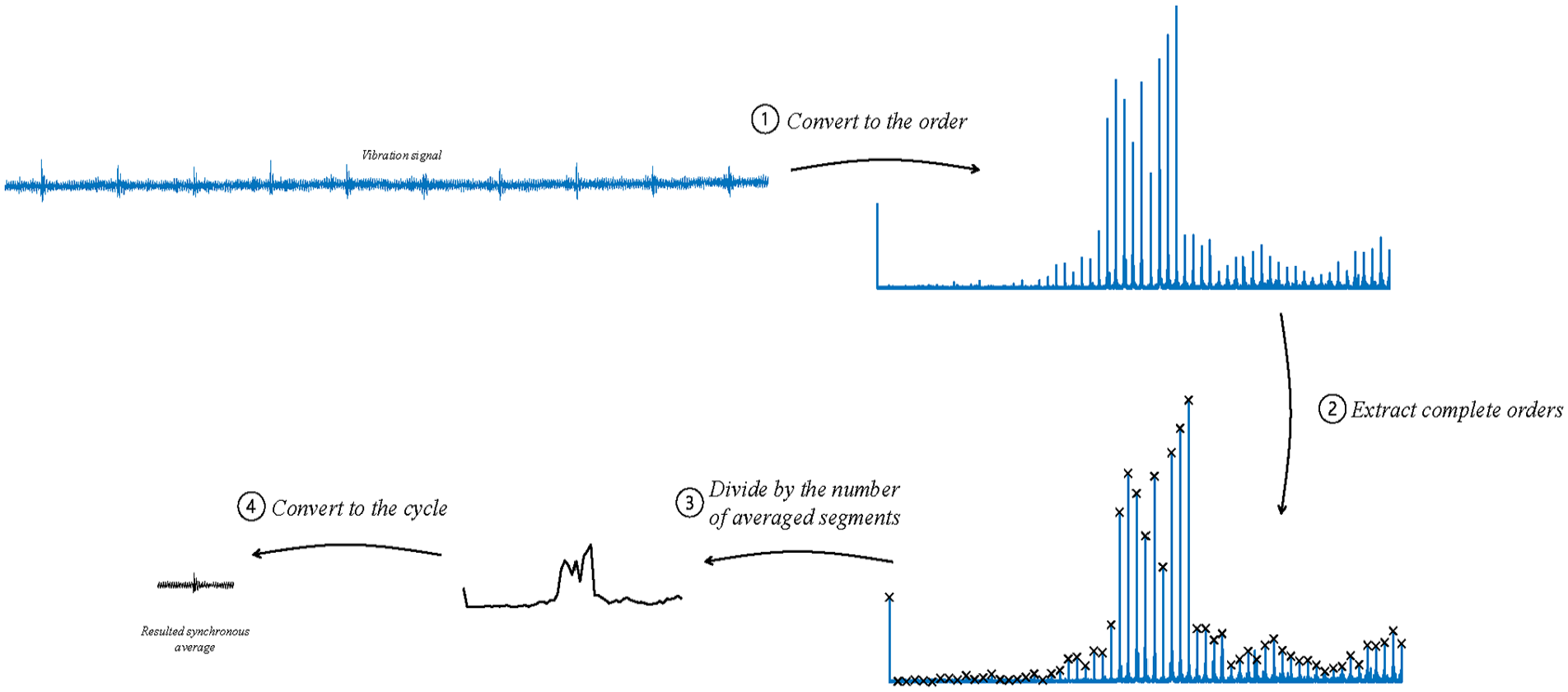
As illustrated in Figure 1, in SA, after angular resampling,^11,12 the signal is divided into consecutive segments, each of them with the length of a complete round. These segments are averaged together.^15,20

Figure 1.

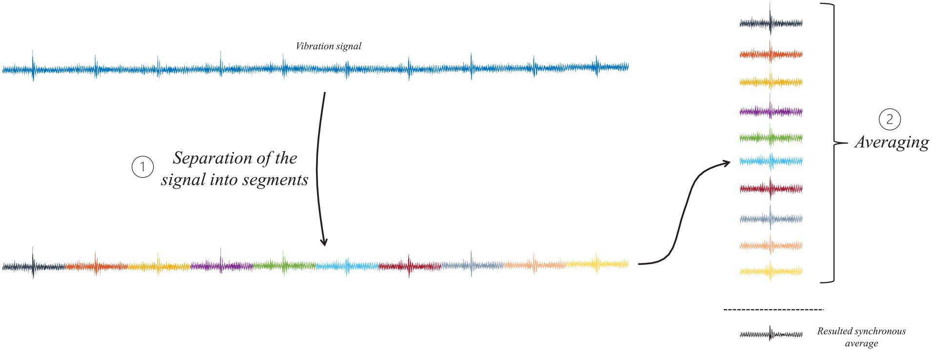
Illustration of SA. SA: synchronous averaging.

SA isolates the vibrations of the component of interest by reducing interferences from other rotating components and random noise, as illustrated in Figure 2. The variance of the random noise is reduced according to 1/M, where $M$ is the number of synchronized segments. This can be proven by following Equation (1), where $sa$ is the calculated SA with $N$ samples, and $sig$ is the signal in the cycle domain with a length of $M \cdot N$ . Assuming the random noises presented in Equation (2), $noise [n], noise [N + n], noise [2 \cdot N + n], \dots noise [(M - 1) \cdot N + n]$ , are independent and identically distributed, we obtain Equation (3), where $σ^{2}$ is the variance of the noise in each sample.²⁴

sa [n] = \frac{1}{M} \sum_{m = 0}^{M - 1} sig [m \cdot N + n]

(1)

sig [m \cdot N + n] = s [m \cdot N + n] + noise [m \cdot N + n]

(2)

\begin{matrix} var (\frac{1}{M} \sum_{m = 0}^{M - 1} noise [m \cdot N + n]) = \frac{1}{M^{2}} \sum_{m = 0}^{M - 1} var \\ (noise [m \cdot N + n]) = \frac{1}{M^{2}} \cdot M \cdot σ^{2} = \frac{σ^{2}}{M} \end{matrix}

(3)

Figure 2.

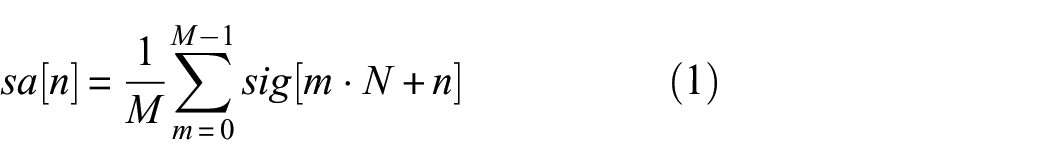
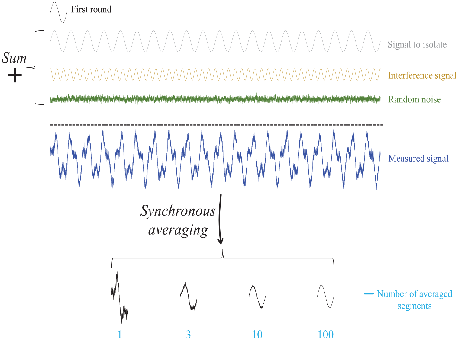
Illustration of the isolation of vibrations of interest by SA, achieved through the reduction of interferences and random noise. SA: synchronous averaging.

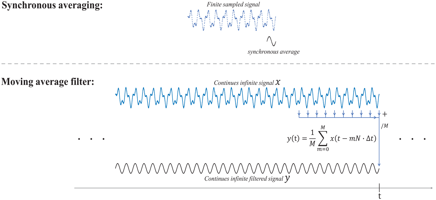
The reduction of interferences from other rotating components requires a slightly more complex analysis. The traditional analysis examines the original infinite continuous signal before the sampling process. According to this analysis, SA can be represented using a moving average filter between the infinite series $x$ and $y$ , as illustrated in Figure 3. $x$ is the original continuous infinite signal from which the signal $sig$ in Equation (1) is sampled, and $y$ is the resulting continuous infinite filtered signal that is merged with the finite vector $sa$ of Equation (1) at the sampled points.

Figure 3.

Analysis of SA as a moving average filter. SA: synchronous averaging.

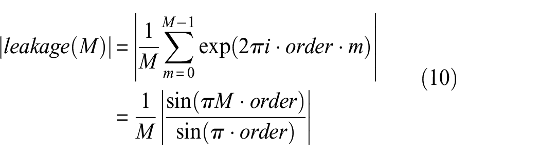
The resulting absolute value of the filter between x and y in the order domain (the frequency domain after angular resampling) is presented in Equation (4), where $order$ is the order value.^15,20 The derivation of Equation (4) is presented in the supporting materials in the first section²⁵:

| H (order) | = | \frac{Y (order)}{X (order)} | = \frac{1}{M} | \frac{\sin (π M \cdot order)}{\sin (π \cdot order)} |

(4)

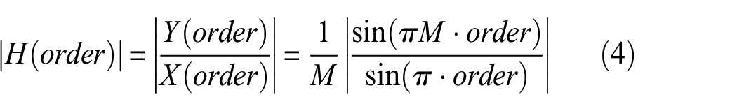
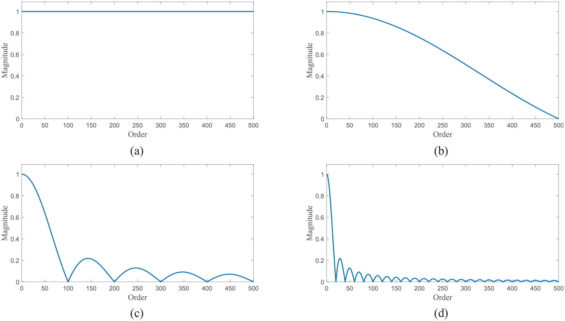
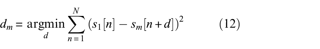
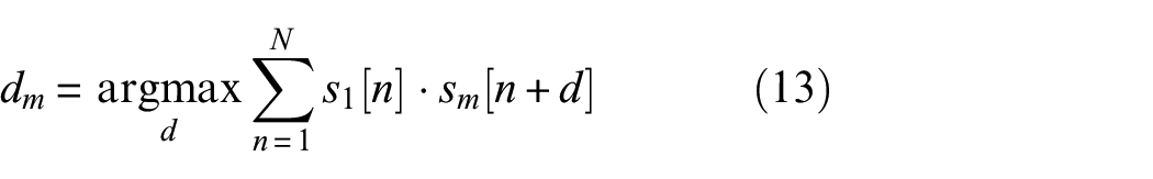
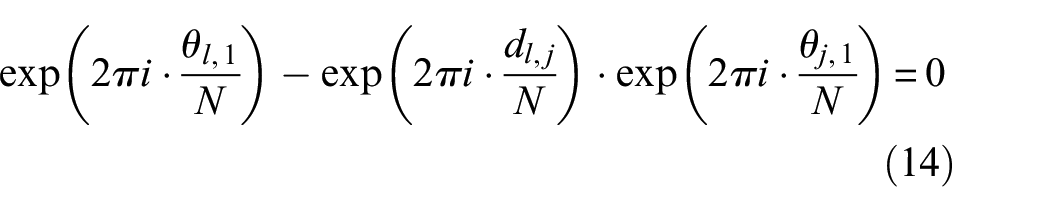
The absolute value of the resulting filter in the order domain is depicted in Figure 4 for an increasing number of averaged segments. As can be seen, the complete orders remain untouched, and all the other orders are attenuated, with several of them even being set to zero. As the number of averaged segments increases, the width of the main lobes becomes tighter, and thus the filter becomes more selective.^10,15

Figure 4.

The resulted filter through SA, concerning the sampled original continuous infinite signal. As the number of averaged segments increases, the filter becomes more selective with respect to the complete orders. (a) The number of averaged segments is 3. (b) The number of averaged segments is 6. (c) The number of averaged segments is 10. (d) The number of averaged segments is 50. SA: synchronous averaging.

It is important to remember that this filter is a continuous filter between the infinite continuous signals $x$ and $y$ and is not directly related to $sig$ and $sa$ of Equation (1). To obtain the SA, we must first sample $y$ and then multiply it by a finite window. This process will have an additional effect on the signal. However, when we want to directly analyze the relation between $sig$ and $sa$ , we are unable to do so using regular filter analysis because they are not even from the same dimension. We will analyze this relation directly in the fourth section.

Figure 5 illustrates the effectiveness of SA in isolating the gear vibration data from the original data.

Figure 5.

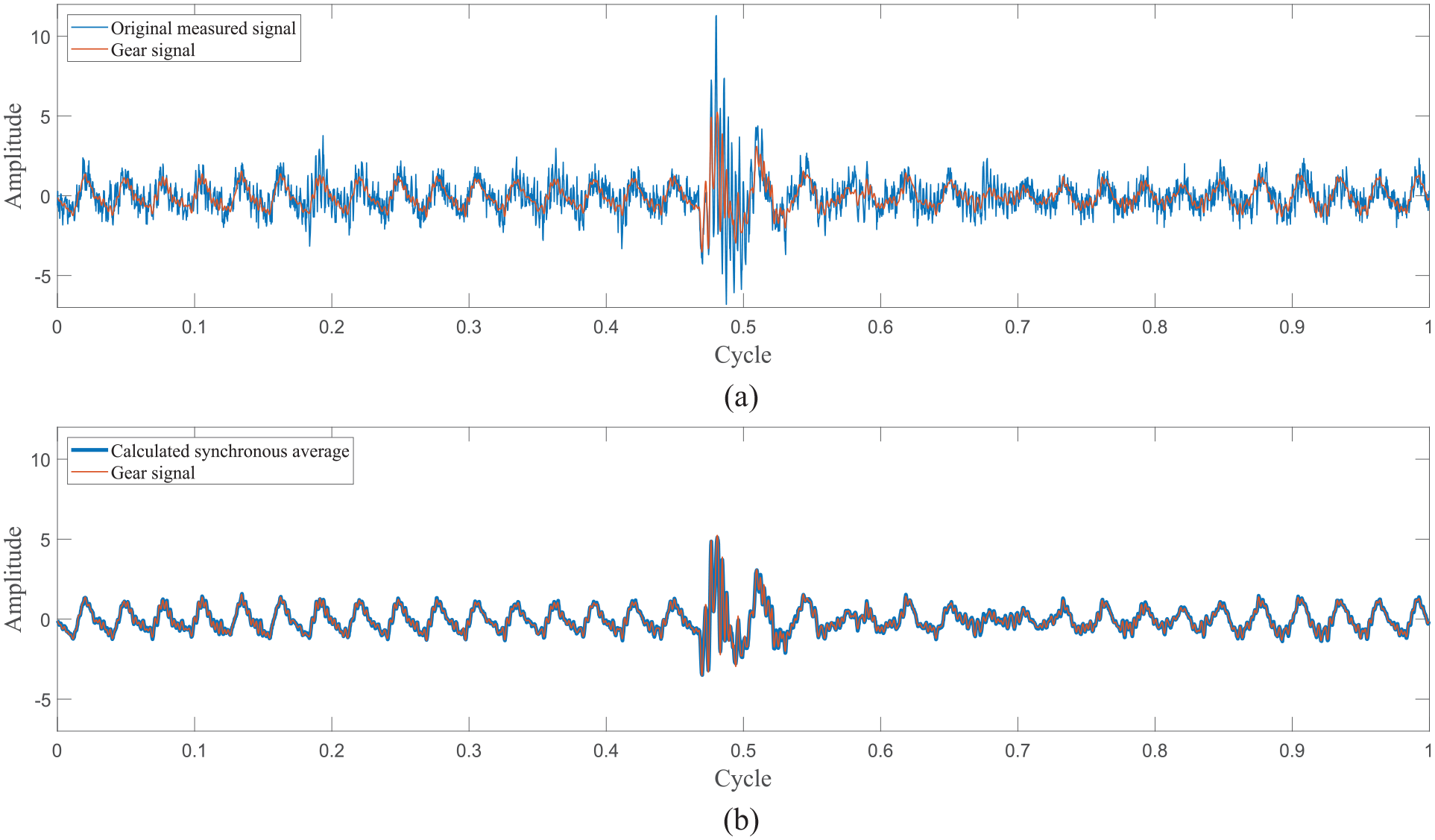
An illustration of the effectiveness of SA in isolating gear vibration. (a) Measured signal. (b) Synchronous average.

Experiments

Four experiments are discussed in this article: one involving a gear fault and three involving bearings with outer race spalls.^26,27 The gear experiment serves to illustrate some of the theoretical analyses and new tools in the fourth section, while the bearing experiments demonstrate the new algorithm described in the sixth section. In this section, these experiments will be described. Table 1 summarizes the experiments conducted. Overall, the new algorithm was tested across three different experiments, nine different loads, two different speeds, and approximately 50 distinct fault types.

Table 1.

Summary of the tested experiments.

Number	Name	Faulted component	Number of records	Description
1	Gear experiment	Gear	14	“Gear experiment” section
2	Endurance	Bearing	40, with two channels	“Endurance bearing experiment” section
3	Monitored	Bearing	30, with two channels	“Monitored spall bearing experiment” section
4	MFPT dataset	Bearing	10	“MFPT dataset” section

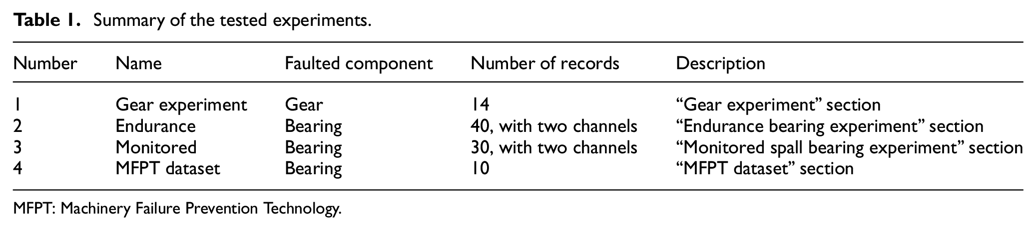
MFPT: Machinery Failure Prevention Technology.

Gear experiment

The gear experiment test rig presented in Figure 6(a) included two spur gears module 3 mm with 35 and 18 teeth, both produced by KHK Gears^TM (Kohara Gear Industry Co., Ltd., Kawaguchi, Japan ). The test rig included also supporting bearings, a speed sensor (magnetic tachometer of Honeywell^TM 3010AN model) (Honeywell International Inc, Charlotte, North Carolina, USA), and a Dytran™ 3053B model accelerometer (Honeywell International Inc, Charlotte, North Carolina, USA). A healthy case and six faults of tooth destruction were tested, as depicted in Figure 6(b). Each health status was tested twice. The motor speed was 45 Hz, the sampling rate of 50 kHz, a load of 10 Nm, and a recording duration of 60 s. A link to the measured data can be found in the Git repository.²⁸

Figure 6.

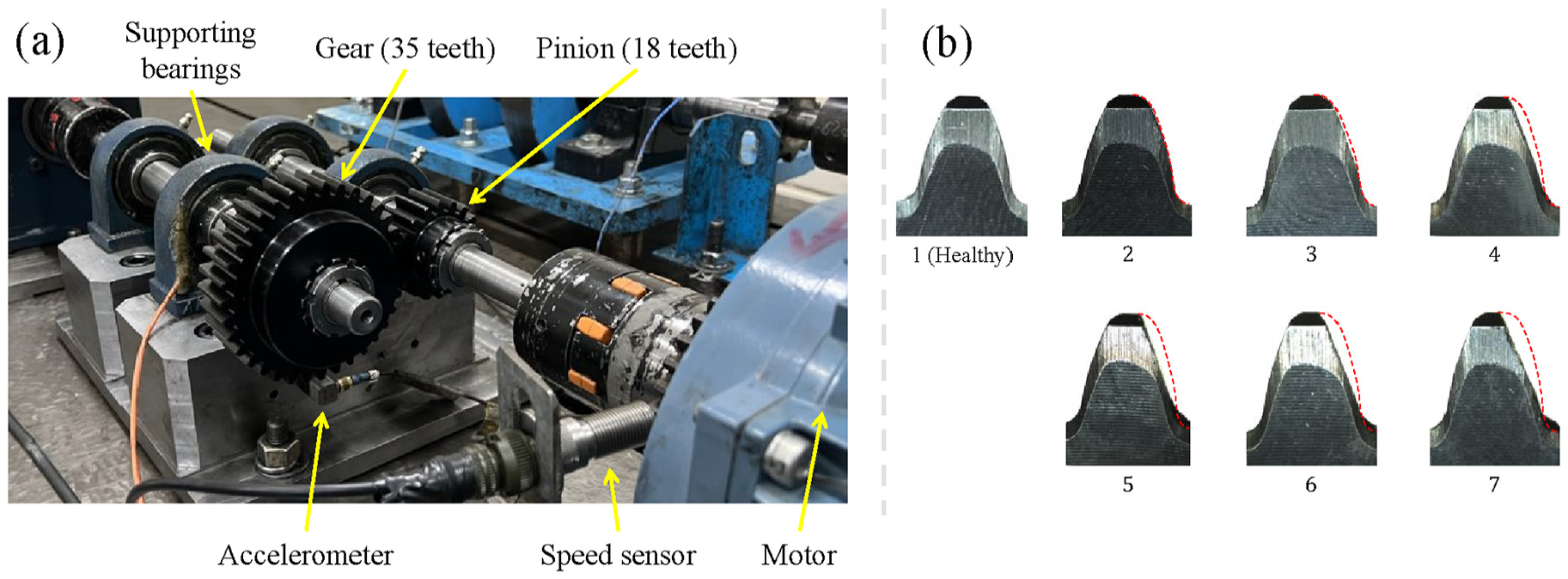
Gear experiment test rig and the seven tested faulted teeth. The vibrations were measured in the gravitational (Z) axis (a) Experiment test rig and (b) Tested faults.

Endurance bearing experiment

The endurance test rig, depicted in Figure 7, included a tested SKF 6206 ETN9 (SKF Group, Gothenburg, Sweden) bearing with an artificially seeded spall, initially shaped as a circle with a diameter of 0.7 mm as depicted in Figure 8. The spall naturally propagated throughout the experiment. The test rig also incorporated supporting bearings and a Dytran™ 3263A2 model accelerometer. The bearing experiment comprised 40 records under speed of 35 Hz with a sampling rate of 50 kHz, and the applied load was 2.2 kN. The records were acquired without disassembling the system. A link to the measured data can be found in the Git repository.²⁸ Each record has a duration of 60 s, and two channels, Z (gravitational) and Y (axial), were tested.

Figure 7.

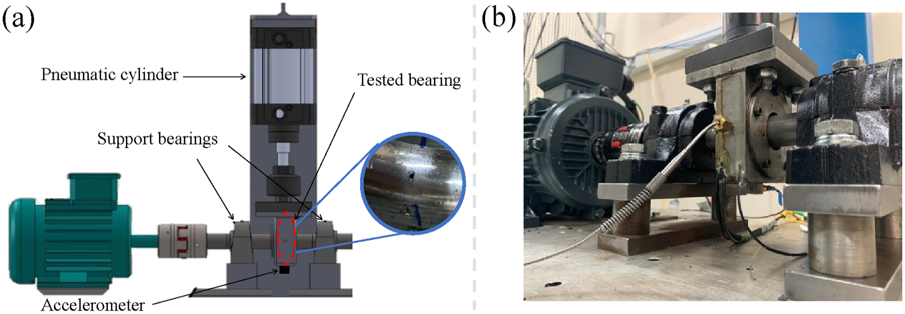
Bearing endurance and monitored spall test rig. (a) Schematic figure and (b) picture of the test rig.

Figure 8.

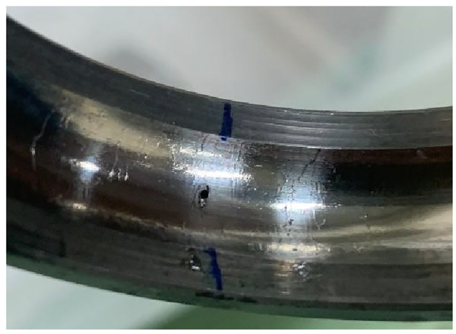
The initial spall in the outer race of the bearing endurance test. The initial spall size was a circle with a diameter of 0.7 mm.

Monitored spall bearing experiment

Another bearing experiment was conducted using the same test rig depicted in Figure 7, which now included six different cases of spalls, with five records for each spall. The initial spall was artificially seeded and shaped as a circle with a diameter of 0.7 mm, as shown in Figure 9. Between each pair of spalls, the system was operated to allow natural propagation and increase the spall size. Subsequently, the system was disassembled to examine the new spall. Images of these spalls throughout the experiment are depicted in Figure 9. The test rig featured a SKF 6206 ETN9 tested bearing and included supporting bearings, as well as a Dytran™ 3263A2 model accelerometer. The bearing experiment comprised 30 records under a speed of 35 Hz with a sampling rate of 50 kHz, and the applied load was 2.2 kN. A link to the measured data can be found in the Git repository.²⁸ Each record has a duration of 60 s, and two channels, Z (gravitational) and Y (axial), were tested.

Figure 9.

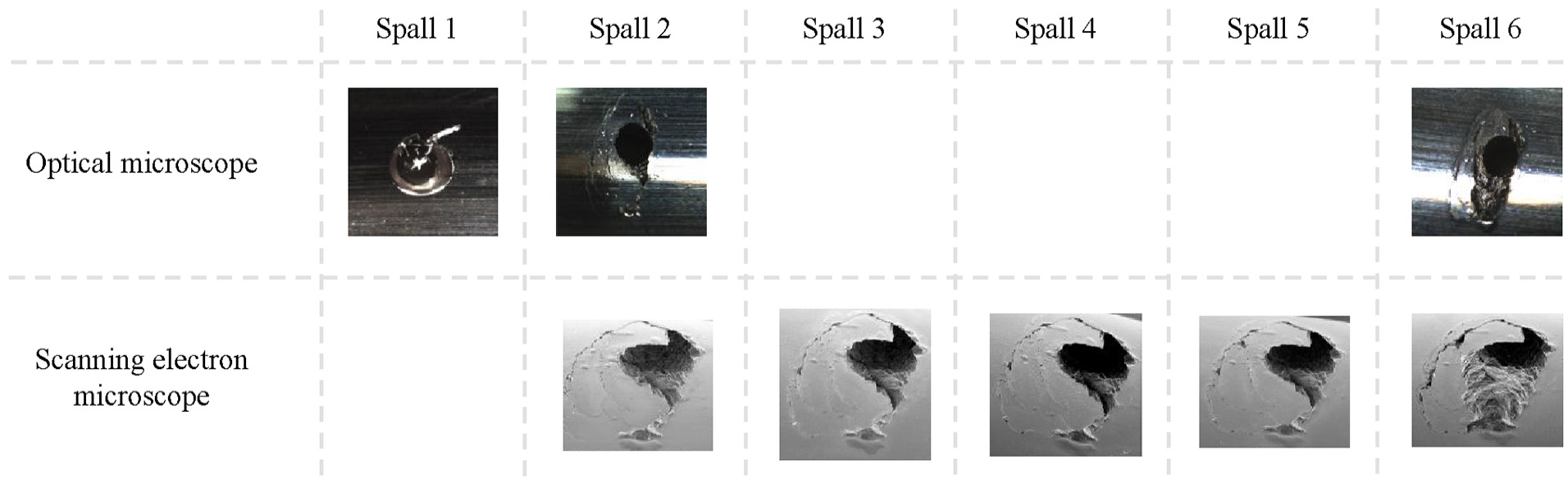
Optical microscope and scanning electron microscope images of the six spalls from the monitored spall test. The initial spall size (spall 1) was a circle with a diameter of 0.7 mm. Spalls 2 and 6 were examined using both options, while spalls 3–5 were examined solely with the scanning electron microscope. Spall 1 was examined using the optical microscope.

MFPT dataset

The Machinery Failure Prevention Technology (MFPT) dataset is a publicly available dataset.²⁹ The dataset has 10 records of bearings with outer race spalls. Three records were collected under a speed of 25 Hz, a sampling rate of 97.656 kHz, a load of 270 lbs, and a duration of 6 s. The remaining seven records were obtained under a speed of 25 Hz, a sampling rate of 48.828 kHz, loads of 25, 50, 100, 150, 200, 250, and 300 lbs, with a duration of 3 s each. The tested bearings were NICE bearings with a roller diameter of 0.235 inch, a pitch diameter of 1.245 inch, eight rolling elements, and a contact angle of zero.

New insights on SA

This section presents new insights into SA. First, it is demonstrated that SA is equivalent to extracting the complete orders from the discrete vector in the order domain of the original signal. Building on this insight, the reduction of interferences is analyzed as a reduction of leakages. A similar analysis will be conducted to mitigate random noise. Both analyses reveal that the reduction of interferences and random noise essentially represents the same phenomenon with two different aspects. Following, two tools, namely the signal-to-noise ratio (SNR) and R² improvement curves, are introduced. The discussion explores how these tools can assist in determining the optimal number of segments to be averaged. It is highlighted that, in the case of gears, it is advisable to use a number of segments that is a complete multiple of the number of teeth on the other wheel. Lastly, a new variation of Simple SA, namely Batch SA, is presented. This technique can enhance performance when the number of segments is not a complete multiple of the teeth on the other wheel.

SA using the order domain

SA is implemented in the cycle domain after angular resampling by averaging the segments, as explained in the second section. This section will elucidate how SA can be calculated using the order. The article presents the final results, with a comprehensive development provided in the supporting materials in the second section.²⁵

The signal $sig$ from Equation (1) can be written using Equation (5), where $a_{k}$ represents its coordinate values after the discrete Fourier transform. The impact of SA on the exponent vectors is analyzed in Equation (6), where $l \cdot M + d = k$ from Equation (5), and $d < M$ . If $d = 0$ , we obtain Equation (7); otherwise, we get Equation (8). Combining these, we derive Equation (9). A more detailed development is presented in the supporting materials in the second section.²⁵ The order resolution of the original signal $sig$ is 1/M; hence, $k \cdot M$ in Equation (9) represents the complete orders.

Thus, as depicted in Figure 10, for calculating the SA using the order domain, the signal is converted to the order domain, and then the values of the complete orders are extracted. After division by the number of averaged segments $M$ , the signal is converted back to the cycle domain.

sig [n] = \frac{1}{M \cdot N} \sum_{k = 0}^{M \cdot N - 1} a_{k} \cdot \exp (2 π i \frac{k \cdot n}{M \cdot N})

(5)

\begin{matrix} \sum_{m = 0}^{M - 1} \exp (2 π i \frac{(l \cdot M + d) (m \cdot N + n)}{M \cdot N}) = \exp \\ (2 π i \frac{(l \cdot M + d) \cdot n}{M \cdot N}) \cdot \sum_{m = 0}^{M - 1} \exp (2 π i \frac{d \cdot m}{M}) \end{matrix}

(6)

\begin{matrix} \exp (2 π i \frac{(l \cdot M) \cdot n}{M \cdot N}) \cdot \sum_{m = 0}^{M - 1} \exp (2 π i \frac{0 \cdot m}{M}) \\ = \exp (2 π i \frac{(l \cdot M) \cdot n}{M \cdot N}) \cdot \sum_{m = 0}^{M - 1} 1 = M \cdot \exp (2 π i \frac{k \cdot n}{M \cdot N}) \end{matrix}

(7)

\begin{matrix} \exp (2 π i \frac{(l \cdot M + d) \cdot n}{M \cdot N}) \cdot \sum_{m = 0}^{M - 1} \exp (2 π i \frac{d \cdot m}{M}) \\ = \exp (2 π i \frac{(l \cdot M + d) \cdot n}{M \cdot N}) \cdot 0 = 0 \end{matrix}

(8)

\begin{matrix} sa [n] = \frac{1}{M} \cdot \sum_{m = 0}^{M - 1} sig [m \cdot N + n] = \frac{1}{M} \cdot \frac{1}{M \cdot N} \sum_{m = 0}^{M - 1} \sum_{k = 0}^{M \cdot N - 1} \\ a_{k} \exp (2 π i \frac{k \cdot (m \cdot N + n)}{M \cdot N}) = \\ = \frac{1}{N} \sum_{k = 0}^{N - 1} \frac{a_{k \cdot M}}{M} \exp (2 π i \frac{k \cdot n}{N}) \end{matrix}

(9)

Figure 10.

Block diagram of SA calculated using the order domain by extracting the complete orders. SA: synchronous averaging.

Reducing interferences and random noise

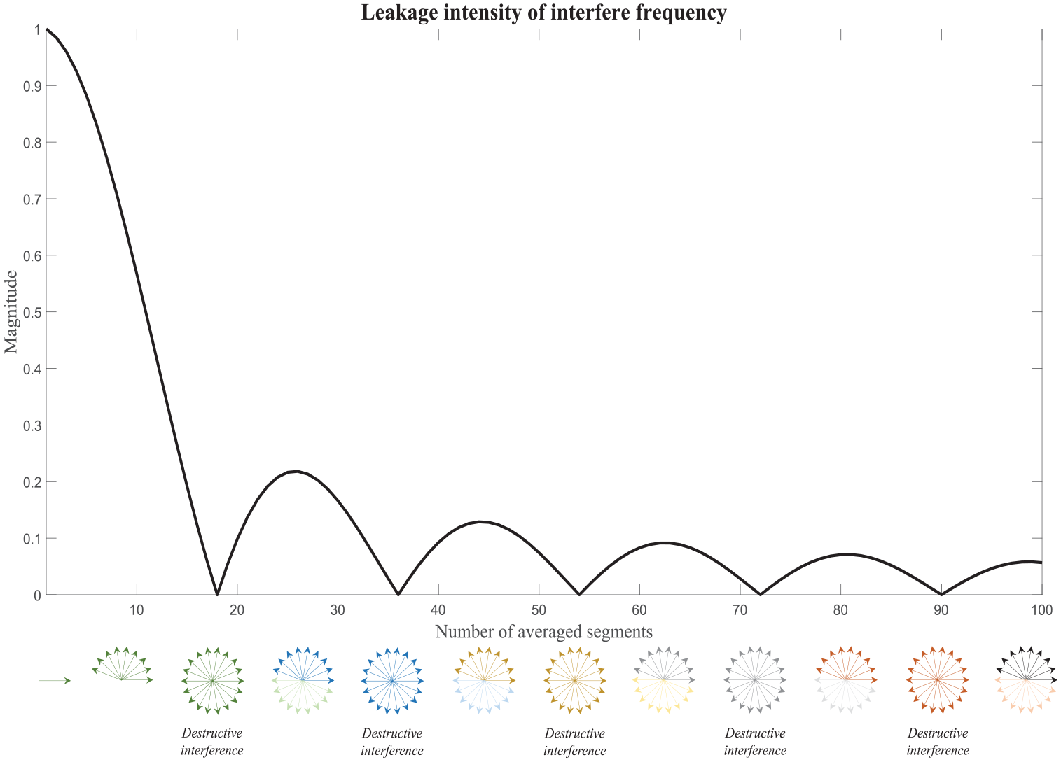
Now, when analyzing SA as extracting complete orders, as depicted in Figure 10, we can consider interferences as leakage into the complete orders. Equation (10) describes the amount of energy that leaks into the complete orders as a function of the number of averaged segments $M$ . Figure 11 illustrates this equation. Not surprisingly, we obtain similar results to Equation (4), where in the current case, the variable is $M$ instead of $order$ .

Figure 11.

An illustration of the leakage intensity of interfere order into the complete orders as function of the number of averaged segments.

Furthermore, we can consider the reduction of interference as follows: when the interference order falls into the coordinate of the original averaged signal $sig$ , it is set to zero because we set the noncomplete orders to zero. Otherwise, it has a leakage, and its intensity is lower when we improve the resolution of the original signal $sig$ in the order domain. As illustrated in Figure 11, we can also consider the behavior of the leakage intensity using destructive interference, where when the interference vector completes round it cancels itself:

\begin{matrix} | leakage (M) | = | \frac{1}{M} \sum_{m = 0}^{M - 1} \exp (2 π i \cdot order \cdot m) | \\ = \frac{1}{M} | \frac{\sin (π M \cdot order)}{\sin (π \cdot order)} | \end{matrix}

(10)

The reduction in random noise is intuitive, as we take only 1/M. of the coordinate in the order, leading to 1/M $\frac{1}{M}$ of the original variance. To provide a more in-depth analysis, contemplate the scenario wherein, for instance, the signal undergoes a transformation from cycle to order and subsequently reverts to order without any form of filtration. Remarkably, despite these alterations, the resultant variance remains unaltered. Presuming the presence of white noise uniformly distributed across the spectrum due to independently and identically distributed original samples, the extraction of only 1/M. of the coordinate results in a proportional reduction, leaving us with 1/M. of the original variance. The supporting materials formalize this intuition in the third section.²⁵

These two analyses, that is, of interferences and random noise, show that the reduction of both stems from the same principle of choosing complete orders and filtering out all the others. The noise is reduced by 1/M. because it is distributed equally across all the orders, while the reduction in interference depends on its order due to the leakage behavior.

SNR and R² curves

For monitoring the performance of SA, we propose two tools: the SNR improvement curve and the R² improvement curve. Both curves monitor the performance of the SA as a function of the number of averaged segments.

Generally speaking, the SNR measures how much the exact selected signal affects the final calculated SA. We would expect that a well-calculated SA will have very low dependency on the exact signal $sig$ from Equation (1) that it is randomly selected from a long record under stationary conditions. Henceforth, when we take a long record and divide it into separate signals, the differences between the calculated SAs of the separate signals can be used to estimate the performance of the SA. Based on this idea, the SNR improvement curve works as follows: for each number of averaged segments $M$ , the long record is divided into separated signals, each of them with a size of $N \cdot M$ ; then, the SA is calculated for each signal. The signal intensity is estimated by the average intensity of the calculated SAs. The noise is estimated based on the mean squared error between the SAs. The SAs are synchronized to eliminate the delay between them (which is important for bearing). An example of a SNR improvement curve of the gear experiment is depicted in Figure 12. In Figure 13, two cases are compared to demonstrate the meaning of low and high SNRs. Two points from Figure 12(a) are depicted: when the number of averaged segments is 1 and 18. As clearly seen in Figure 13, when the SNR is high, the exact signal from the long record that is used to calculate the SA has little effect on the final result.

Figure 12.

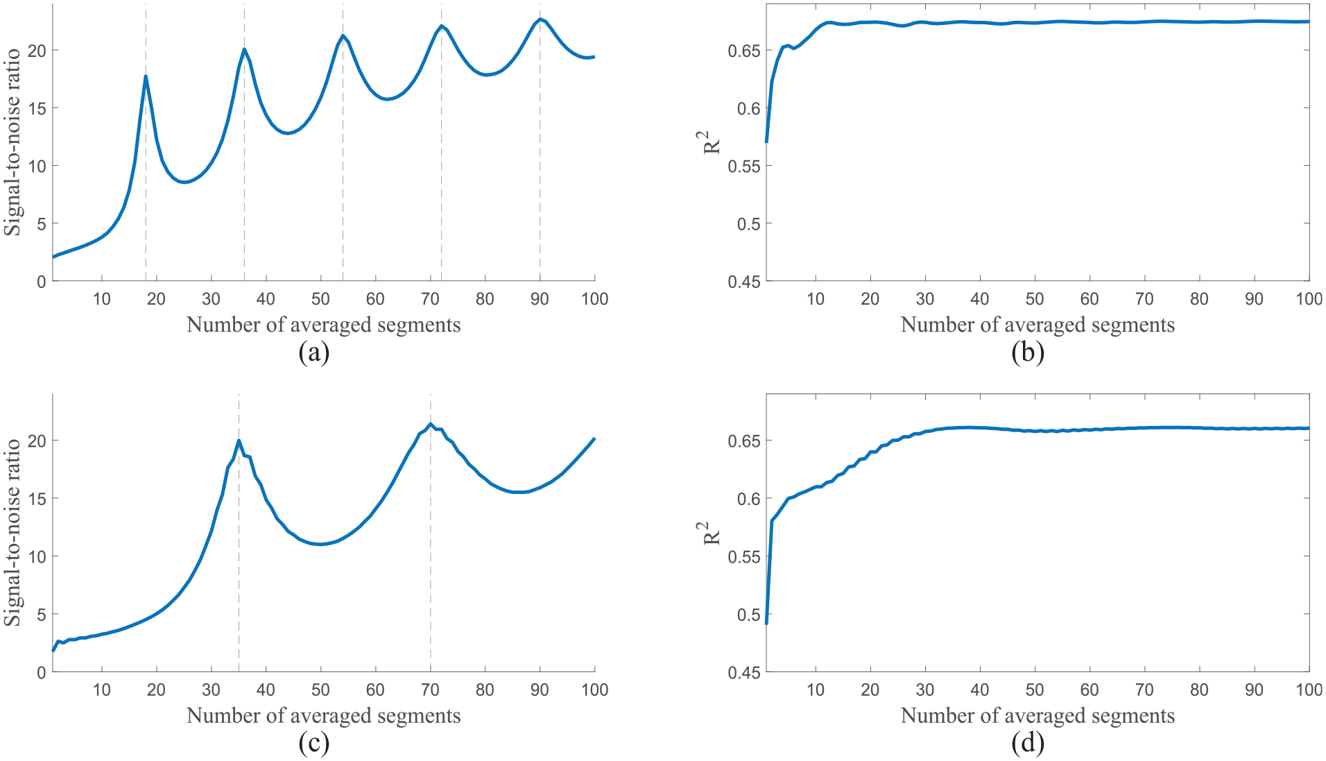
An example of SNR and R² improvement curves for a measured record from the gear experiment. The dashed gray line in (a) represents the multiplication by 18, and in (c), it represents the multiplication by 35. (a) SNR improvement curve, gear. (b) R² improvement curve, gear. (c) SNR improvement curve, pinion. (d) R² improvement curve, pinion. SNR: signal-to-noise ratio.

Figure 13.

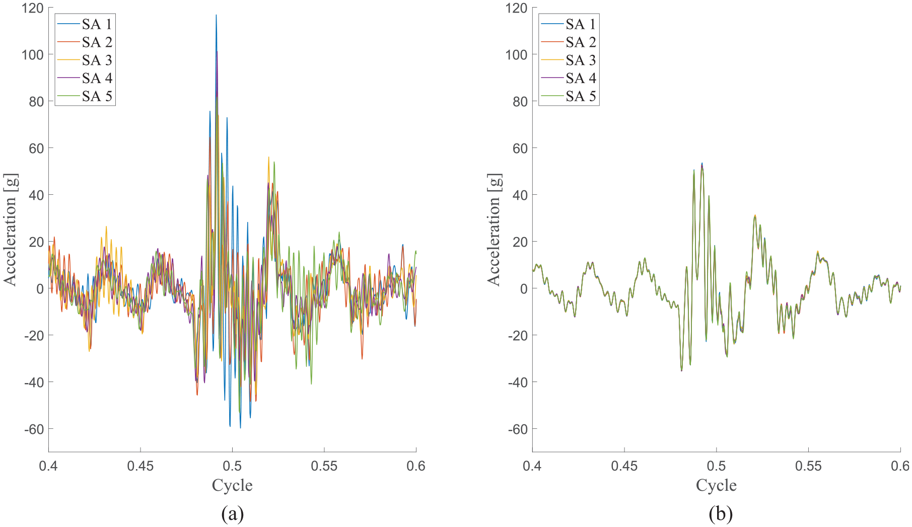
An example of a (a) low SNR and (b) high SNR based on the case presented in Figure 12(a); due to high SNR SA 5 in (b) covers all the other SAs. (a) 1 averaged segments. (b) 18 averaged segments. SA: synchronous averaging; SNR: signal-to-noise ratio.

The R² improvement curve measures how much of the noise in the original record the calculated SA explains. For each number of averaged segments $M$ , one SA is calculated from the long record. Then, the record is divided into consecutive segments, each of them with the length of the SA, $N$ . For each segment, the SA and the segment are synchronized, and the mean squared error ( $ms e_{error}$ ) is calculated. The R² of each segment is calculated by $\frac{1 - ms e_{error}}{ms e_{sgmnt}}$ , where $ms e_{sgmnt}$ is the mean squared error of the segment. The estimated R² of the segments are averaged together. Figure 12 demonstrates the R² improvement curve. The importance of this curve is to validate that the SA does not output a degenerated signal with a good SNR, for example, a constant signal that is not dependent on the input. It is less important than the SNR improvement curve.

These two curves can serve three purposes: validating that the SA works without problems (e.g., significant errors in the speed measurement for the angular resampling), enabling the choice of the optimal number of averaged segments—in this case, a complete multiplication of the number of teeth on the other wheel—and also indicating how many segments should be regarded until a sufficiently good SNR is achieved.

Other wheel phenomenon and Batch SA

The SNR and R² improvement curves were employed to assess the gear experiment. As depicted in Figure 12, for both the gear and pinion, when the number of averaged segments equals the number of teeth on the other wheel, the SNR reaches a local maximum. This phenomenon repeats across all tested records, as illustrated in the supporting materials in the fourth section.²⁵ It demonstrates the destructive interference phenomenon presented in Figure 11.

We propose a new technique for enhancing Simple SA, which we designate as Batch SA. According to this technique, as illustrated in Figure 14, the record is separated into two overlapping signals, each having a length equal to the complete multiplication of segments by the number of teeth on the other wheel. This allows, on the one hand, to utilize all the data to reduce noise and, on the other hand, to leverage the destructive interference phenomenon to eliminate the influence of the other wheel. This technique is beneficial in cases where the number of segments in a record is not a complete multiplication of the teeth on the other wheel. For instance, when there are 30 teeth on the other wheel and the record consists of 50 segments. Figure 15 reproduces the scenario presented in Figure 12, demonstrating how Batch SA improves Simple SA for cases where the number of segments is not a complete multiplication. Additional examples from the gear experiment are provided in the supporting materials in the fourth section.²⁵

Figure 14.

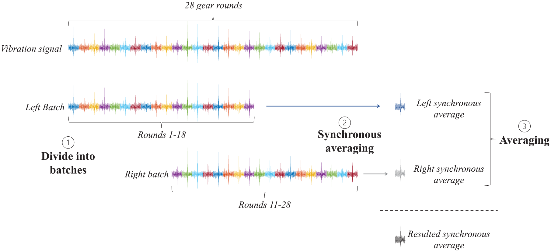
Block diagram of Batch SA. The number of teeth on the other wheel in this case is 18. SA: synchronous averaging.

Figure 15.

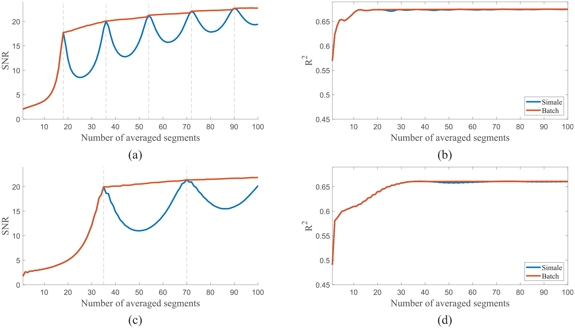
An example of SNR and R² improvement curves for a measured record from the gear experiment that is also presented in Figure 12. The dashed gray line in (a) represents multiplication by 18, and in (c), it represents multiplication by 35, which are the number of teeth on the other wheel in each case. (a) SNR improvement curve, gear. (b) R² improvement curve, gear. (c) SNR improvement curve, pinion. (d) R² improvement curve, pinion. SNR: signal-to-noise ratio.

Figure 15 compares the performance of Batch SA and Simple SA in subfigures (a) and (c), across different numbers of averaged segments. As shown in the figure, when the number of averaged segments is between 1 and the number of teeth on the other gear, both algorithms perform identically, since they are essentially executing the same operation. However, immediately beyond that range, the performance of Simple SA declines due to interference from the signal of the other gear. Simple SA exhibits a sinusoidal-like performance pattern that depends on how close the number of averaged segments is to the number of teeth on the interfering gear. In contrast, Batch SA shows consistently improving performance that does not depend on the number of teeth on the other gear; therefore, when the number of averaged segments differs from the number of teeth on the other gear, Batch SA outperforms Simple SA. This performance advantage becomes especially significant when the number of averaged segments lies closely between two multiples of the other gear’s tooth count. For example, in Figure 15(c), when the number of averaged segments is 50, Batch SA achieves an SNR of approximately 20 dB, compared to only 10 dB for Simple SA—a performance improvement of nearly 10 dB.

The generalized problem and theoretical analysis

Concerning a set of several numbers, the mean squared error metric induces the average as the number that is closest to all the other numbers in the set. Consequently, the SA can be viewed as the solution to the problem of finding the signal for which the mean squared error between it and all segments of the signal is minimized. SA be generalized to a broader problem in which we seek the SA for which the mean squared error between it and the segments of the signal is minimal, accounting for delays of the segments, as illustrated in Figure 16. This generalized problem is suitable for scenarios like bearings, where the segments are not perfectly synchronized due to random fluctuations. This general problem is Nondeterministic Polynomial (NP)-hard.³⁰

Figure 16.

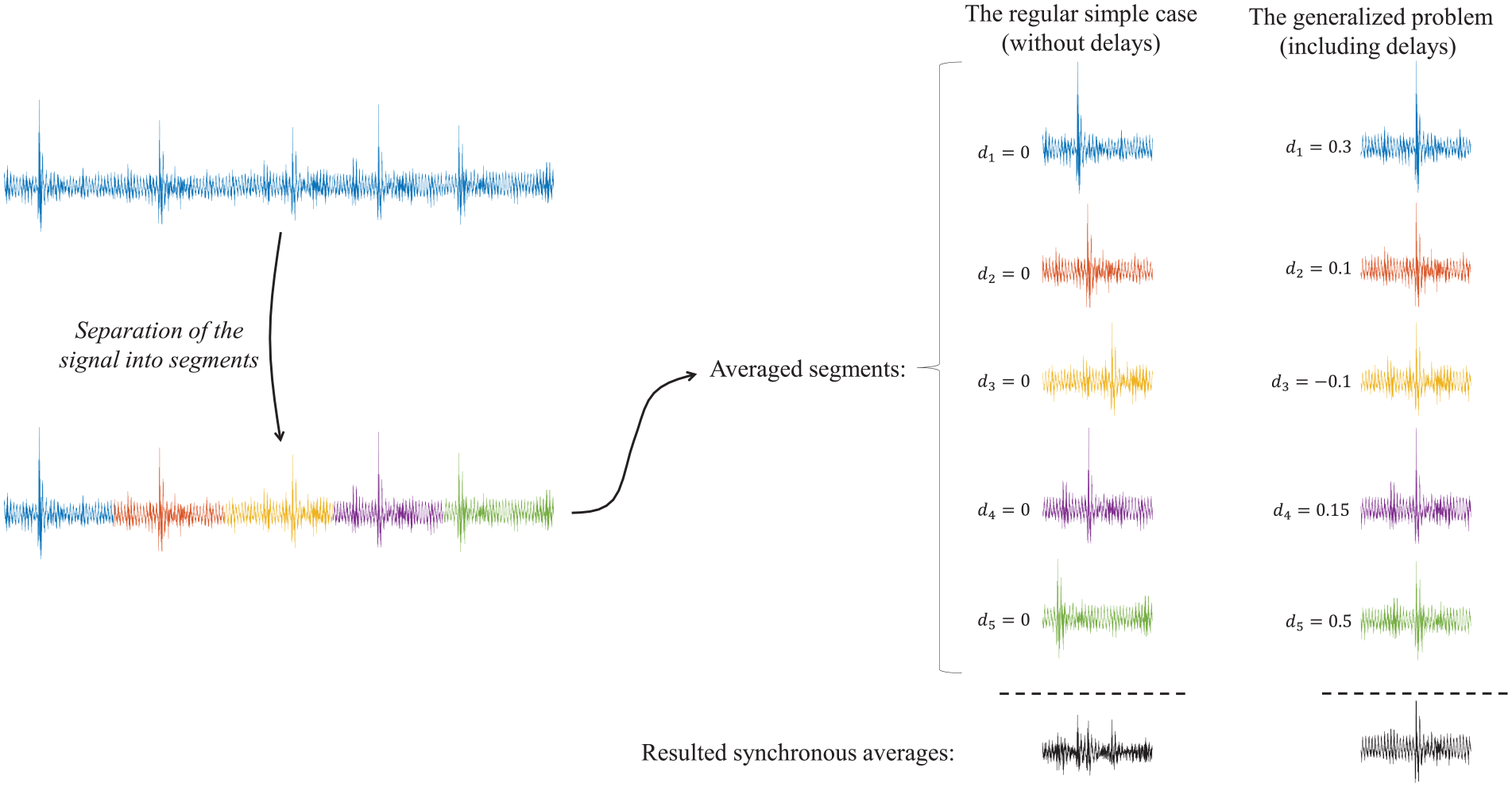
An illustration of the generalized problem in which delays between the calculated SA and the segments of the signal are allowed. SA: synchronous averaging.

For Simple SA, where the segments are simply averaged together, the effects of delays on the calculated SA can be analyzed as a low-pass filter. The calculated SA represents the desired SA with delays between the averaged segments, as illustrated in Figure 17(a). The delay transformation between the desired SA and each segment is linear and circularly invariant. Furthermore, the averaging of the segments is also linear and circularly invariant. Therefore, all transformation from the desired SA to the calculated one is linear and circularly invariant, equivalent to multiplying the desired SA in the order domain by a filter, as illustrated in Figure 17(b).

Figure 17.

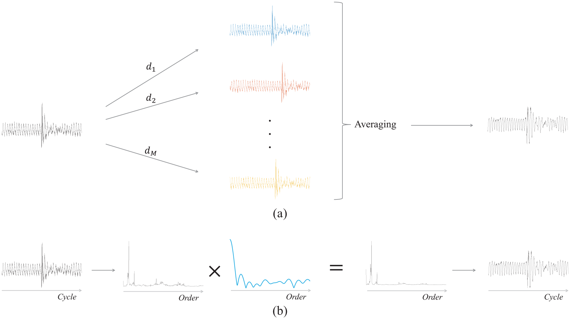
Illustration of the equivalence between the effect of the delays on the SA in the cycle due to averaging of different segments with delays and filtering in the order domain. The delays between the segments create a low-pass filter. SA: synchronous averaging.

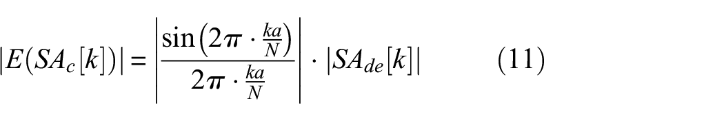
Equation (11) presents the magnitude of the expected value of the $k$ coordinate of the calculated SA ( $S A_{c} [k]$ ) in the order domain due to random delays with a uniform distribution $U [- a, a]$ ,³¹ where $N$ is the number of points in the SA (the development of this equation is given in the supporting materials in the fifth section²⁵ based on the law of the unconscious statistician³²). As can be observed, it forms a low-pass filter between the desired SA ( $S A_{de} [k]$ ) and the calculated one ( $S A_{c} [k]$ ), where a wider distribution variance results in a narrower low-pass filter. Figure 18 depicts the magnitude of the expected filter for a uniform distribution with increased variance. This observation indicates that, because of fluctuations, Simple SA is incapable of isolating the high orders of the desired signal, and this issue becomes more pronounced when the fluctuations are stronger. This phenomenon is, of course, not restricted solely to a uniform distribution of delays; it is applicable to a broader range, including distributions such as the normal distribution. As we will see in the seventh section, for bearing vibrations, this phenomenon results in the inability of Simple SA to isolate the desired bearing signal at all:

| E (S A_{c} [k]) | = | \frac{\sin (2 π \cdot \frac{ka}{N})}{2 π \cdot \frac{ka}{N}} | \cdot | S A_{de} [k] |

(11)

Figure 18.

Demonstration of the random delays on the filter between the desired SA and the calculated Simple SA. When the variance of the delays distribution is larger the low-pass filter is narrower. (a) Delay ~ U[0,0]. (b) Delay ~ U[−0.1%,+0.1%]. (c) Delay ~ U[−0.5%,+0.5%]. (d) Delay ~ U[−2.5%,+2.5%]. SA: synchronous averaging.

The new algorithm Angular Synchronization SA

The new algorithm, Angular Synchronization SA, is illustrated in Figure 19. The algorithm consists of three steps:

The measured signal is divided into consecutive segments, and these segments are then synchronized to the first segment, $s_{1}$ . This is achieved by finding the delay $d_{m}$ between each segment $s_{m}$ and $s_{1}$ through the minimization of the mean squared error, as depicted in Equation (12). Instead of using $O (N^{2})$ computational running time, this can be computed more efficiently using Equation (13) with a computational running time of $O (N \cdot \log (N))$ when discrete Fourier transform is used. Not surprisingly, it reminds cross-correlation. Based on the estimated delays the segments are averaged together:

d_{m} = \underset{d}{argmin} \sum_{n = 1}^{N} {(s_{1} [n] - s_{m} [n + d])}^{2}

(12)

d_{m} = \underset{d}{argmax} \sum_{n = 1}^{N} s_{1} [n] \cdot s_{m} [n + d]

(13)

Averaging Synchronizing iterations are used to enhance the calculated SA. The delays between the segments and the calculated SA are estimated again according to Equation (12), and then the synchronized segments are averaged together. These iterations are repeated K times. This operation improves the mean squared error between the segments and the calculated SA in each iteration. Initially, when the delays between the segments and the calculated SA are estimated, the mean squared error between the synchronized segments and the SA naturally decreases. Subsequently, when a new SA is calculated, the mean squared error decreases again because the averaging operation returns the vector with the minimal mean squared error between it and all the averaged segments.

Small delays between the segments are rectified using “equal votes” from all segments. Initially, delays between all the segments are estimated within a maximal deviation restriction, such as 1%. Subsequently, the delays between the first segment and all other segments ( $θ_{l, 1}$ and $θ_{j, 1}$ ) are estimated by solving Equation (14) using the least squares method, as suggested by Singer,³³ where $d_{l, j}$ is the estimated delay between the $l_{th}$ segment and the $j_{th}$ segments. This technique allows the utilization of information from all segments to enhance the accuracy of delay estimation. The segments are then synchronized based on the estimated delays and averaged together:

\exp (2 π i \cdot \frac{θ_{l, 1}}{N}) - \exp (2 π i \cdot \frac{d_{l, j}}{N}) \cdot \exp (2 π i \cdot \frac{θ_{j, 1}}{N}) = 0

(14)

Figure 19.

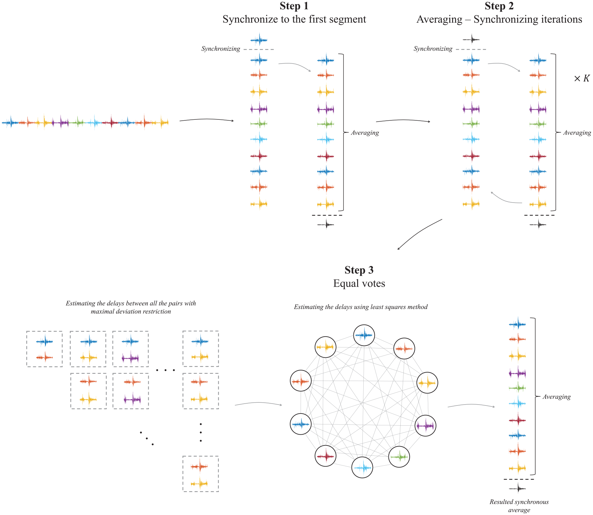
Block diagram of the new algorithm, Angular Synchronization SA, for bearing vibrations. SA: synchronous averaging.

Examination on experimental data

In this section, the new algorithm, Angular Synchronization SA, is first compared to Simple SA. All three bearing experiments are used for quality comparison. The two experiments with 60-second records, endurance and monitored tests, enable quantitative comparison in addition to the qualitative one. Following this, the contributions of the three different steps of the new algorithm are demonstrated.

In all cases the number of averaging synchronizing iterations were $K = 10$ and the maximal deviation in step 3 was 1%. The number of averaged segments in the endurance and monitored spall tests was 500 while due to shorter record duration it was 90 in the MFPT dataset.

Comparison of the new algorithm and Simple SA

Figures 20 and 21 present the results of the new algorithm and Simple SA on the endurance and monitored spall tests. The quantitative results show a significant improvement in all cases. Figures 22, 24, 25, and 26 depict several examples of the calculated SAs from the endurance test, monitored spall test, and MFPT dataset for qualitative comparison. It is clearly evident that while Simple SA is unable to estimate the bearing SA, the new algorithm accomplishes this clearly for all cases. More examples are provided in the supporting materials in the sixth section.²⁵

Figure 20.

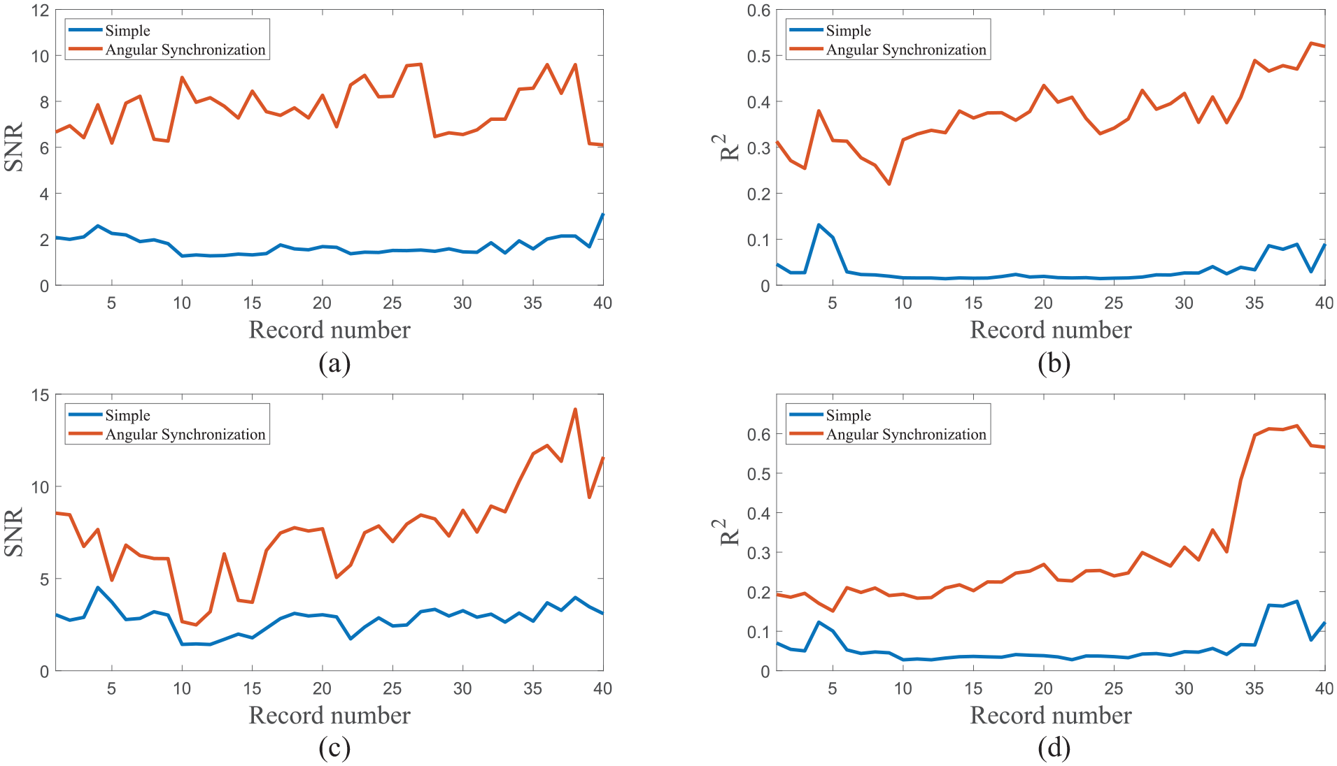
Comparison of the new algorithm and Simple SA on the endurance test. (a) Endurence test, Z axis. (b) Endurence test, Z axis. (c) Endurence test, Y axis. (d) Endurence test, Y axis. SA: synchronous averaging.

Figure 21.

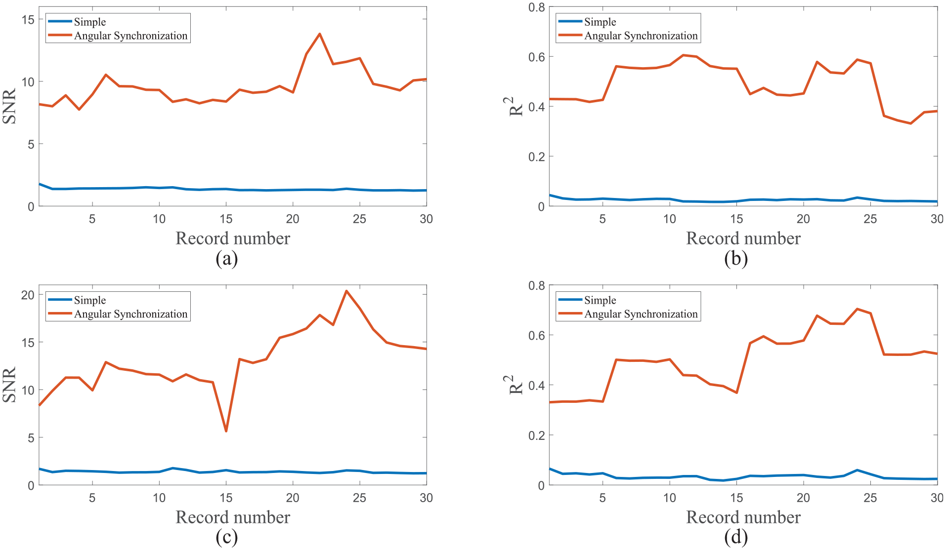
Comparison of the new algorithm and Simple SA on the monitored test. (a) Monitored test, Z axis. (b) Monitored test, Z axis. (c) Monitored test, Y axis. (d) Monitored test, Y axis. SA: synchronous averaging.

Figure 22.

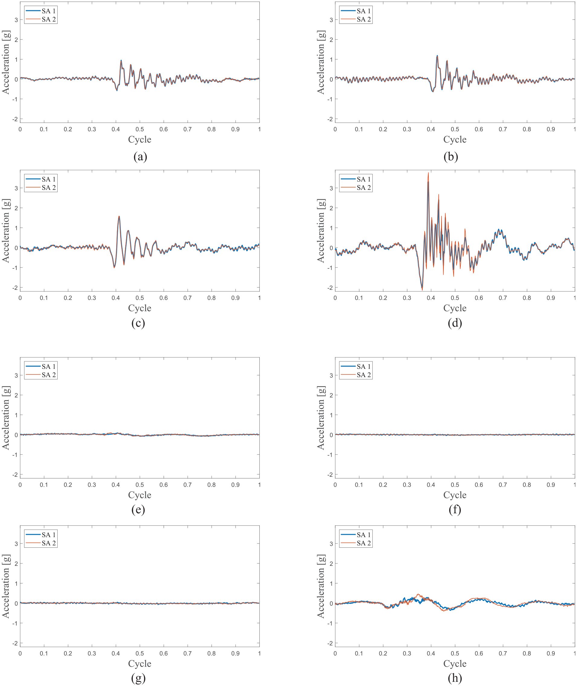
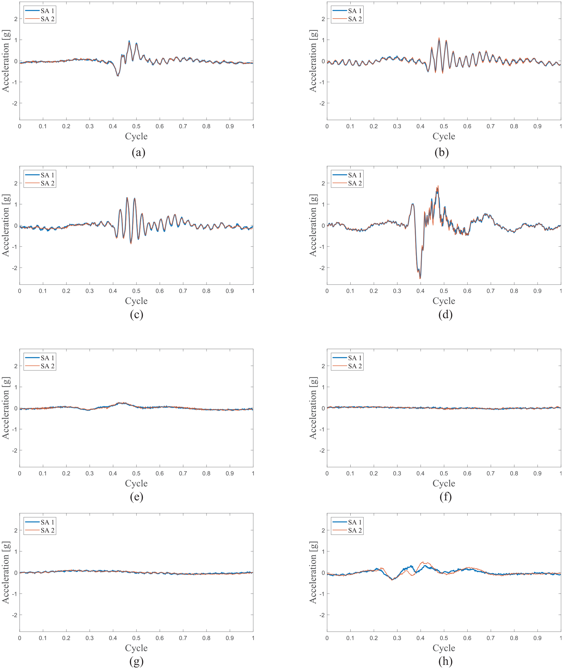
Comparison of calculated SAs of the new algorithm and Simple SA on the endurance test, Z axis. (a) Angular Synchronization SA, record number 1. (b) Angular Synchronization SA, record number 14. (c) Angular Synchronization SA, record number 27. (d) Angular Synchronization SA, record number 40. (e) Simple SA, record number 1. (f) Simple SA, record number 14. (g) Simple SA, record number 27. (h) Simple SA, record number 40. SA: synchronous averaging.

Figure 23.

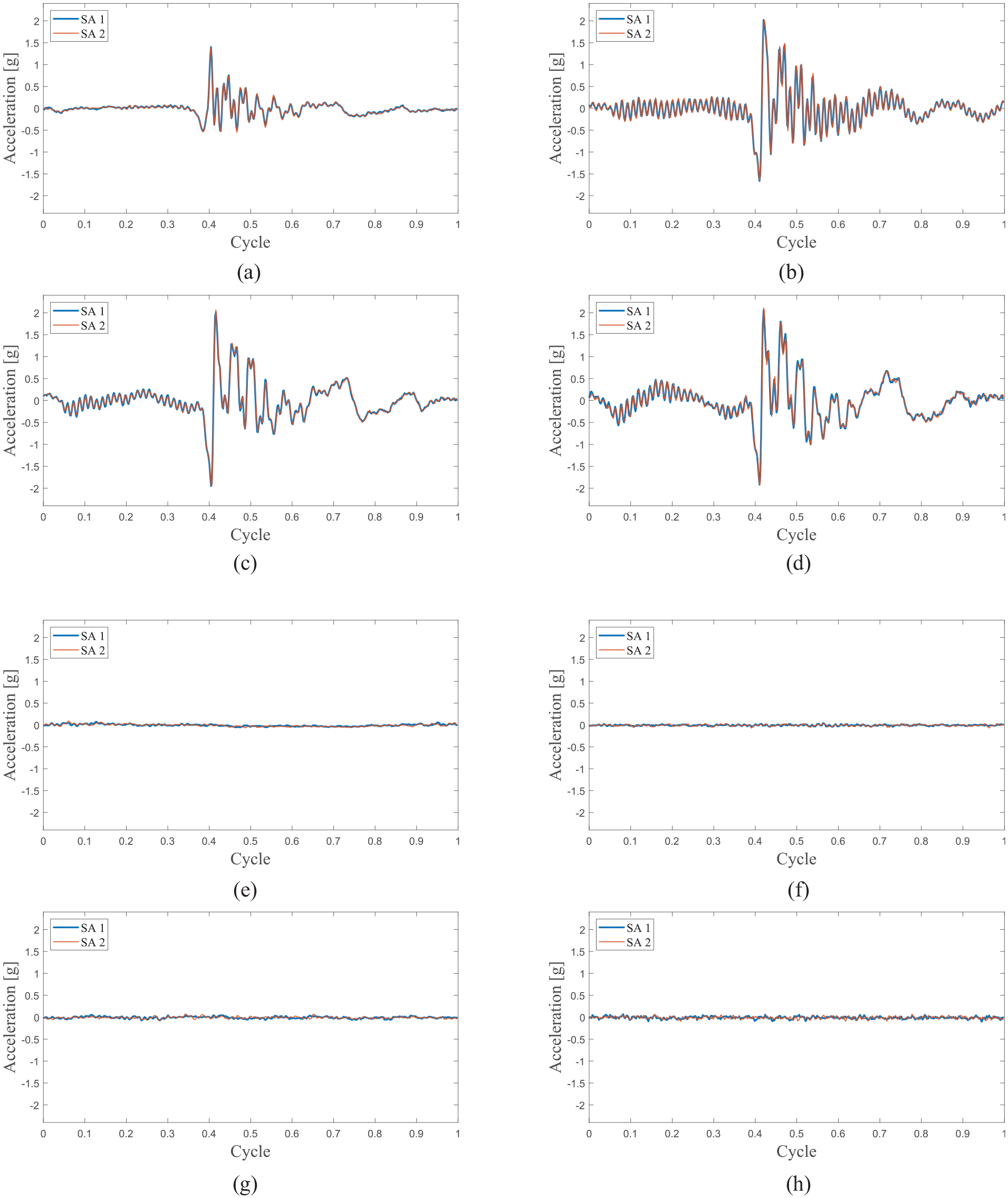
Comparison of calculated SAs of the new algorithm and Simple SA on the endurance test, Y axis. (a) Angular Synchronization SA, record number 1. (b) Angular Synchronization SA, record number 14. (c) Angular Synchronization SA, record number 27. (d) Angular Synchronization SA, record number 40. (e) Simple SA, record number 1. (f) Simple SA, record number 14. (g) Simple SA, record number 27. (h) Simple SA, record number 40. SA: synchronous averaging.

Figure 24.

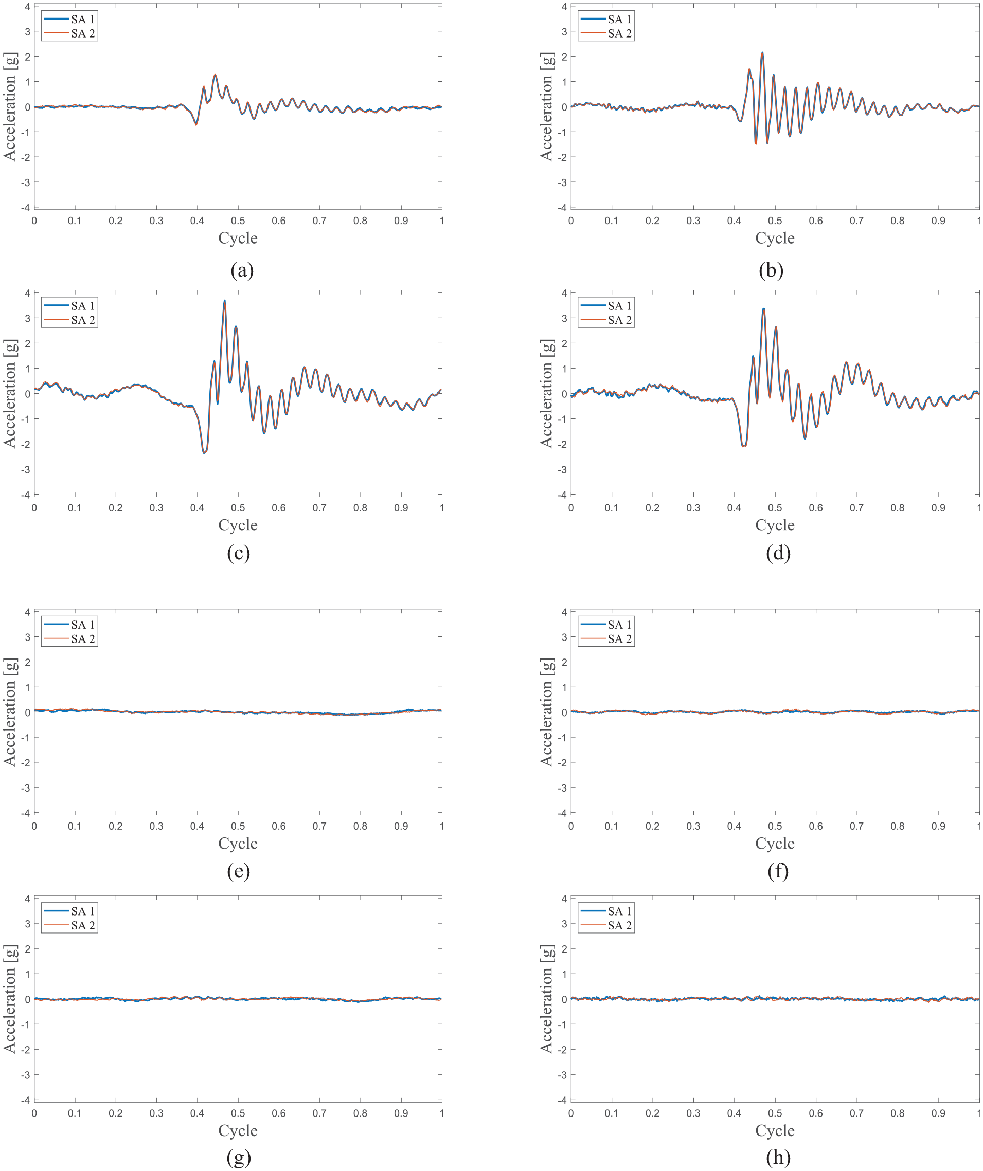
Comparison of calculated SAs of the new algorithm and Simple SA on the monitored test, Z axis. (a) Angular Synchronization SA, record number 1. (b) Angular Synchronization SA, record number 11. (c) Angular Synchronization SA, record number 21. (d) Angular Synchronization SA, record number 30. (e) Simple SA, record number 1. (f) Simple SA, record number 11. (g) Simple SA, record number 21. (h) Simple SA, record number 30. SA: synchronous averaging.

Figure 25.

Comparison of calculated SAs of the new algorithm and Simple SA on the monitored test, Y axis. (a) Angular Synchronization SA, record number 1. (b) Angular Synchronization SA, record number 11. (c) Angular Synchronization SA, record number 21. (d) Angular Synchronization SA, record number 30. (e) Simple SA, record number 1. (f) Simple SA, record number 11. (g) Simple SA, record number 21. (h) Simple SA, record number 30. SA: synchronous averaging.

Figure 26.

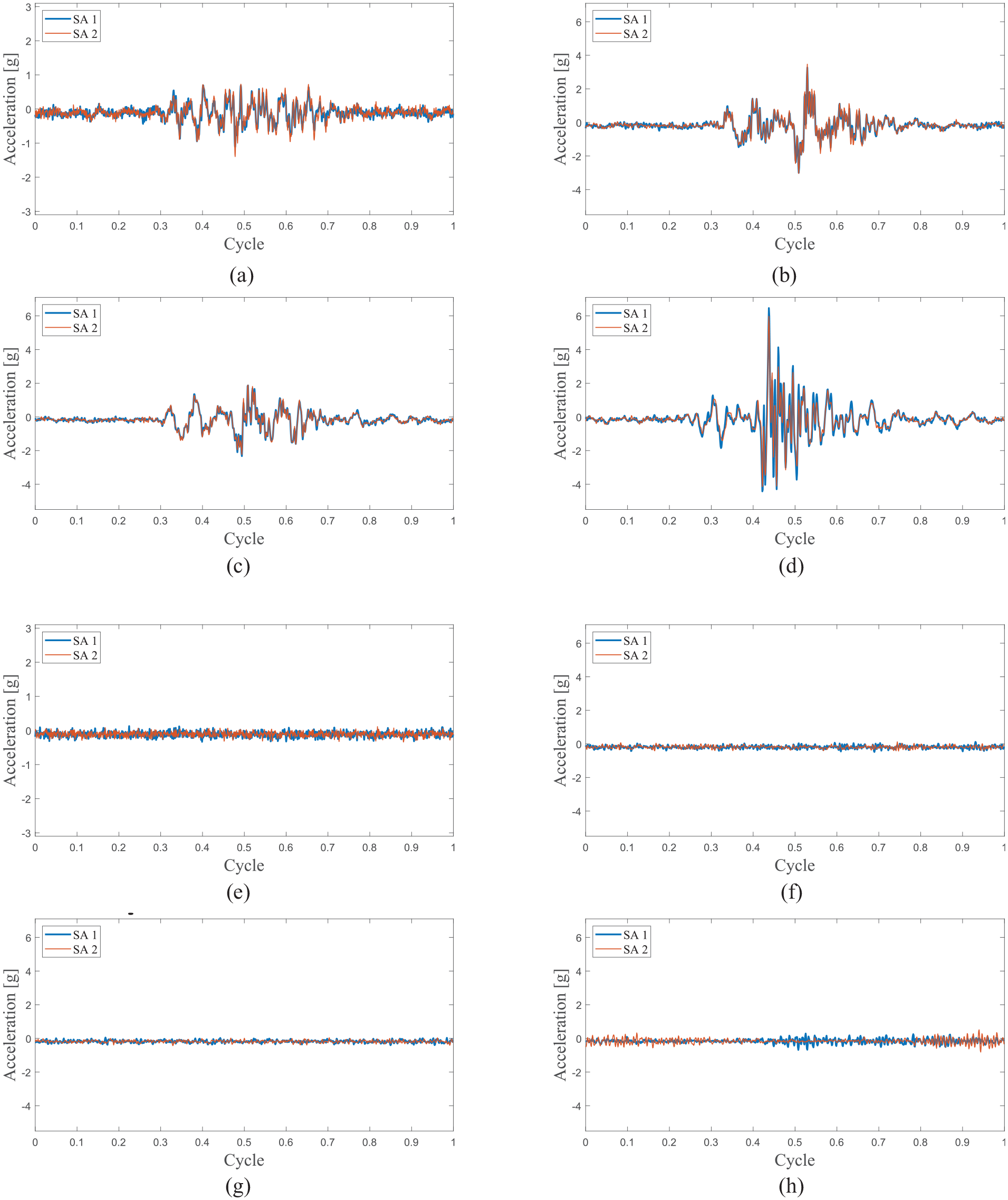
Comparison of calculated SAs of the new algorithm and Simple SA on the MFPT dataset. (a) Angular Synchronization SA, record number 1. (b) Angular Synchronization SA, record number 4. (c) Angular Synchronization SA, record number 7. (d) Angular Synchronization SA, record number 10. (e) Simple SA, record number 1. (f) Simple SA, record number 4. (g) Simple SA, record number 7. (h) Simple SA, record number 10. SA: synchronous averaging.

Bearing signals inherently exhibit speed fluctuations due to the slipping of the roller elements relative to the outer or inner races. Accordingly, all the bearing experiments in our study include such fluctuations, which the proposed algorithm—Angular Synchroni-zation SA—is designed to overcome. This is demonstrated by the comparison with Simple SA, which fails to handle these fluctuations effectively. As demonstrated in Figures 20 to 26, Simple SA is unable to estimate the signal due to the presence of speed fluctuations, whereas the proposed Angular Synchronization SA successfully manages to do so.

In Figure 22(h), an example of the low-pass filter effect of Simple SA is evident. In this case, part of the SA is estimated, and as can be seen, it is composed from low frequencies. This can be simply explained by the analysis in the fifth section, where it is shown that the delays between the segments create a low-pass filter effect on the Simple SA.

The currently available algorithm, Simple SA, has a computational complexity of $O (N \cdot M)$ , where $N$ is the number of samples per segment and $M$ is the number of averaged segments. However, its performance is very poor, as shown in Figures 20 to 26. From a quantitative perspective, Simple SA performs poorly in almost all cases, with a SNR typically ranging between 1 and 3 dB (Figures 20 and 21). This is significantly lower than the SNR achieved by the proposed Angular Synchronization SA algorithm. Qualitatively, as shown in Figures 22 to 26, Simple SA always fails to estimate the SA, producing either zero-valued outputs or heavily smoothed signals, unlike the more accurate results obtained with Angular Synchronization SA.

Although Angular Synchronization SA has a higher computational complexity of $O (NlogN \cdot M \cdot K + NlogN \cdot M^{2})$ where $K$ is the number of iterations, it demonstrates substantially better performance. Based on the results in Figures 22 to 26, it is clear that Simple SA is generally unsuitable for estimating the SA of bearing signals, while Angular Synchronization SA provides reliable estimations.

Examination of the components of the new algorithm

Figure 27 presents the quantitative results for the three stages of the new algorithm. The R² curves are not provided, as they do not offer additional interesting information. As seen in the figure, in most cases, the averaging-synchronizing iterations make a significant contribution to step 1, synchronization with the first segment. This is a very reasonable result because synchronizing to the first segment gives too much importance to the first segment over all the others. After using the average to estimate the delays, all segments have the more importance. Second, we can consider synchronizing to the first segments as a smart guess for the averaging-synchronizing iterations. Instead of initiating the iterations with random delays or the original delays, we actually begin by assuming the first segment as the SA and then estimate the delays regularly. Hence, the mean squared error is improved, and the algorithm’s performance after the averaging synchronizing iterations is better. In many cases, the last step improves the results. As explained in the sixth section, the “equal vote” enables the removal of a lot of noise. Furthermore, the last stage can also provide noncomplete integer delays, allowing us to refine the solution.

Figure 27.

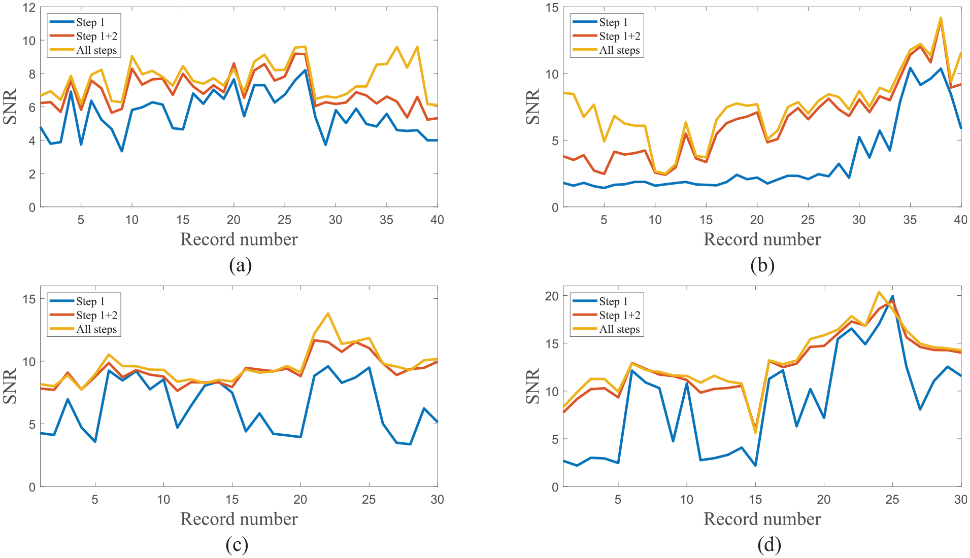
Contribution of the three steps of the new algorithm to the final results on the endurance and monitored tests. (a) Endurence test, Z axis. (b) Endurence test, Y axis. (c) Monitored test, Z axis. (d) Monitored test, Y axis.

The final step of the new algorithm involves computing the delays between all segments. Consequently, when the number of segments is large, it is significantly slower than just using steps 1 and 2. We recommend using all steps when running time is not an issue and using steps 1 and 2 when it is. That said, due to the self-checkability of the algorithm with the SNR, it is always possible to run the algorithm with both options on several tested cases of the system and choose the one that provides sufficient performance while running in a reasonable time.

Summary

In this article, we analyze the SA process and introduce a new algorithm that enables its application to bearing vibrations. We begin by reviewing the current knowledge about it and demonstrate that reducing interference and random noise both result from the same operation of extracting the complete orders regarding the discrete problem. We present new tools for monitoring performance and show how the suggested Batch SA can enhance performance for gears. Next, we recognize the SA problem as a more generalized problem of minimizing the mean square error with respect to delays between segments. We provide a theoretical analysis of the effects of the delay on SA. Based on this generalized problem, we propose a new algorithm, Angular Synchronization SA, for calculating the SA of bearing vibrations, by estimating the delay between segments. We demonstrate the ability of the new algorithm in comparison to Simple SA through three experiments.

Future research can extend the current work in several directions. First, the newly proposed algorithm, Angular Synchronization SA, can be applied to additional cases. Furthermore, the three steps—synchronization to the first segment, averaging-synchronization iterations, and fine delay estimation using equal voting—can be expanded into more refined stages to further improve algorithm performance. The new algorithm enables estimation of the SA, which is particularly important for many gear diagnostics algorithms. The demonstrated ability to estimate the SA in bearings, as shown in this article, opens up opportunities for future research on bearing diagnostics, including severity estimation and remaining useful life prediction based on SA.

Supplemental Material

sj-docx-1-shm-10.1177_14759217251350962 – Supplemental material for Novel approaches of synchronous averaging of gear and bearing vibrations

Supplemental material, sj-docx-1-shm-10.1177_14759217251350962 for Novel approaches of synchronous averaging of gear and bearing vibrations by Omri Matania, Roee Cohen, Lior Bachar, Eric Bechhoefer and Jacob Bortman in Structural Health Monitoring

Footnotes

Declaration of conflicting interests

The author(s) declared no potential conflicts of interest with respect to the research, authorship, and/or publication of this article.

Funding

The author(s) disclosed receipt of the following financial support for the research, authorship, and/or publication of this article: Omri Matania is supported by the Adams Fellowships Program of the Israel Academy of Sciences and Humanities.

Declaration of generative AI and AI-assisted technologies in the writing process

During the preparation of this work the authors used ChatGPT 3.5 exclusively to improve readability and language. After using this tool, the authors meticulously reviewed and edited the content as needed and take full responsibility for the content of the publication.

ORCID iDs

Omri Matania

Roee Cohen

Lior Bachar

Jacob Bortman

Data availability statement

All the codes and data used in this paper, including the explanation video and supporting materials file, are available via the Git repository

Supplemental material

Supplemental material for this article is available online.

References

Stewart

RM.

Some useful data analysis techniques for gearbox diagnostics. In: Proceedings of the meeting on the applications of time series analysis, ISVR. Southampton, UK, https://books.google.co.il/books/about/Some_Useful_Data_Analysis_Techniques_for.html?id=owf_MgEACAAJ&redir_esc=y (1977, accessed 24 November 2023).

McFadden

Smith

JD.

A signal processing technique for detecting local defects in a gear from the signal average of the vibration. Proc Inst Mech Eng C J Mech Eng Sci 1985; 199: 287–292.

Wang

McFadden

PD.

Decomposition of gear motion signals and its application to gearbox diagnostics. J Vib Acoust 1995; 117: 363–369.

Wang

Wong

AK.

Autoregressive model-based gear fault diagnosis. J Vib Acoust 2002; 124: 172–179.

Matania

Zamir

Bortman

A new tool for model examination: estimation of the mediator transfer function between the model and measured signals. J Sound Vib 2023; 548: 117560.

Kundu

Darpe

Kulkarni

MS.

A review on diagnostic and prognostic approaches for gears. Struct Health Monit 2021; 20: 2853–2893.

Feng

Chen

, et al. A cyclostationarity-based wear monitoring framework of spur gears in intelligent manufacturing systems. Struct Health Monit 2023; 22: 3092–3108.

Wang

An evaluation of some emerging techniques for gear fault detection. Struct Health Monit 2003; 2: 225–242.

Randall

. Section 5.3.1: Time synchronous averaging. In: Vibration-based condition monitoring: industrial, automotive and aerospace applications. Hoboken, NJ: Wiley, 2021, pp. 178–180.

10.

Braun

( Simon

). Chapter 6: Time domain averaging (synchronous averaging). In: Discover signal processing: an interactive guide for engineers. Hoboken, NJ: Wiley, 2008, pp. 265–269.

11.

Villa

Reñones

Perán

, et al. Angular resampling for vibration analysis in wind turbines under non-linear speed fluctuation. Mech Syst Signal Process 2011; 25: 2157–2168.

12.

Order analysis based on resampling – national instruments, https://www.ni.com/docs/en-US/bundle/diadem/page/genmaths/genmaths/calc_oa_resampling.htm (accessed 16 October 2022).

13.

Tofighi Niaki

Alavi

Ohadi

. Incipient fault detection of helical gearbox based on variational mode decomposition and time synchronous averaging. Struct Health Monit 2023; 22: 1494–1512.

14.

Feng

, et al. A novel vibration indicator to monitor gear natural fatigue pitting propagation. Struct Health Monit 2023; 22: 3126–3140.

15.

Braun

The extraction of periodic waveforms by time domain averaging. Acustica 1975; 32: 69–77.

16.

McFadden

PD.

A revised model for the extraction of periodic waveforms by time domain averaging. Mech Syst Signal Process 1987; 1: 83–95.

17.

Braun

( Simon

). Section 6.2: Time domain averaging (TDA). In: Mechanical signature analysis: theory and applications. Cambridge, MA: Academic Press, 1986, pp. 142–149.

18.

Vachtsevanos

Lewis

Roemer

, et al. Section 4.3.4: Time synchronous averaging (TSA). In: Intelligent fault diagnosis and prognosis for engineering systems. Hoboken, NJ: Wiley, 2006, pp. 101–104.

19.

Bechhoefer

Kingsley

. A review of time synchronous average algorithms. In: Annual conference of the prognostics and health management society, PHM 2009. pp. 1–10.

20.

Braun

The synchronous (time domain) average revisited. Mech Syst Signal Process 2011; 25: 1087–1102.

21.

Silva

HAP

Nicoletti

. Rotor vibration control using tilting-pad journal bearing with active pads — numerical and experimental results. J Sound Vib 2023; 546: 117441.

22.

Liu

, et al. Vibration analysis of the propulsion shaft system considering dynamic misalignment in the outer ring. J Sound Vib 2024; 589: 118612.

23.

Matania

Dattner

Bortman

, et al. A systematic literature review of deep learning for vibration-based fault diagnosis of critical rotating machinery: limitations and challenges. J Sound Vib 2024; 590: 118562.

24.

Blitzstein

Hwang

. Section 4.6: Variance. In: Introduction to probability. 2nd ed. Boca Raton: CRC Press, pp. 171–174.

25.

Supporting materials for the paper ‘Novel approaches of synchronous averaging of gear and bearing vibrations’, https://github.com/omriMatania/novel_approaches_of_synchronous_averaging_of_gear_and_bearing_vibrations (accessed 26 November 2023).

26.

Epps

McCallion

. An investigation into the characteristics of vibrations excited by discrete faults in rolling element bearings. In: Vibrations association of New Zealand (VANZ) 1st annual conference. Rotorua, 1991.

27.

Epps

. An investigation into vibration excited by discrete faults in rolling element bearing. PhD thesis, University of Canterbury, 1991.

28.

Git repository of the paper ‘Novel approaches of synchronous averaging of gear and bearing vibrations’, https://github.com/omriMatania/novel_approaches_of_synchronous_averaging_of_gear_and_bearing_vibrations (accessed 26 November 2023).

29.

MFPT. Fault data sets, https://www.mfpt.org/fault-data-sets (2012, accessed 26 November 2023).

30.

Bandeira

Charikar

Singer

, et al. Multireference alignment using semidefinite programming. In: ITCS 2014 – Proceedings of the 2014 Conference on Innovations in Theoretical Computer Science. Madison, NJ: Association for Computing Machinery, pp. 459–470.

31.

Blitzstein

Hwang

. Section 5.2: Uniform. In: Introduction to probability. 2nd ed. Boca Raton, FL: CRC Press, 2019, pp. 220–223.

32.

Blitzstein

Hwang

. Section 4.5: Law of the unconscious statistician (LOTUS). In: Introduction to probability. 2nd ed. Boca Raton, FL: CRC Press, 2019, pp. 170–171.

33.

Singer

Angular synchronization by eigenvectors and semidefinite programming. Appl Comput Harmon Anal 2011; 30: 20–36.

Supplementary Material

Please find the following supplemental material available below.

For Open Access articles published under a Creative Commons License, all supplemental material carries the same license as the article it is associated with.

For non-Open Access articles published, all supplemental material carries a non-exclusive license, and permission requests for re-use of supplemental material or any part of supplemental material shall be sent directly to the copyright owner as specified in the copyright notice associated with the article.

0.00 MB

2.96 MB

Novel approaches of synchronous averaging of gear and bearing vibrations

Abstract

Keywords

Introduction

Theoretical background

Experiments

Gear experiment

Endurance bearing experiment

Monitored spall bearing experiment

MFPT dataset

New insights on SA

SA using the order domain

Reducing interferences and random noise

SNR and R2 curves

Other wheel phenomenon and Batch SA

The generalized problem and theoretical analysis

The new algorithm Angular Synchronization SA

Examination on experimental data

Comparison of the new algorithm and Simple SA

Examination of the components of the new algorithm

Summary

Supplemental Material

sj-docx-1-shm-10.1177_14759217251350962 – Supplemental material for Novel approaches of synchronous averaging of gear and bearing vibrations

Footnotes

Declaration of conflicting interests

Funding

Declaration of generative AI and AI-assisted technologies in the writing process

ORCID iDs

Data availability statement

Supplemental material

References

Supplementary Material

SNR and R² curves