Sage Journals: Discover world-class research

Abstract

Recently, composite brake blocks have been widely adopted in European railway systems to replace cast iron brake blocks in order to reduce braking noise. However, the poor heat dissipation of composite materials has caused more wheel tread damage, including wheel flats (WFs). The WF, as an undesirable tread defect in railway vehicles, can cause severe wheel/rail impact and increase the damage probability of wheelset components and track structures. Early detection of WFs is vital to ensure operational safety and reduced maintenance costs. In this work, to help understand the dynamic impact caused by WFs, a single WF with a length of 20 mm is artifically produced on a wheel of a tank wagon, and field experiments are performed. The influence of the WF on the axle box accelerations (ABAs), vertical accelerations of the bogie frame and vertical accelerations of the car body is discussed in the time and time-frequency domains. On the other hand, the angular domain synchronous averaging (ADSA) method is used to detect WFs by averaging the ABA signals in the angular domain over a fixed time interval, and it requires ABA data and the axle rotational speed as inputs. This method can greatly reduce the amount of measured data by averaging it in the angle domain and can eliminate the short-time influence of interference signals caused by switches and crossings, rail joints, and so on. The results show that the ADSA of a defective wheel with the WF has a clear peak with an amplitude of 21–104 m/s² while that of a healthy wheel fluctuates around zero in the polar coordinate. Also, the waveform of defective signals can be well presented in polar coordinates. The effectiveness of this method is compared with the envelope spectrum technology in three scenarios and its application to three journeys is presented.

Keywords

Wheel flat detection dynamic impact experimental study angular domain synchronous averaging axle box acceleration

Introduction

Wheel flat (WF) is one of the most common wheel surface defects for railway vehicles, and it is caused by improper braking or poor wheel-rail adhesion due to environmental adversities (rain, snow, oil, etc.), which leads to the wheel sliding on the rail.^1,2 The WFs could induce extreme impact forces between the wheel and the rail in the high-frequency bands, which can cause severe damage to wheelset components^3–6 and the track structure.^7–9 For example, WFs could increase the damage probability of bearings and axles, and they can also promote the development of wheel cracks and wheel wear. Bian et al.⁸ studied the dynamic wheel/rail impact forces caused by WFs by developing a three-dimensional finite element model in ANSYS, and the results showed that the presence of WFs significantly increases the dynamic impact forces on both rails and sleepers. Xu et al.¹⁰ discussed the effect of WFs on dynamic wheel-rail impact in railway turnouts, and the results showed that the wheel with a WF crossing the frog area excites greater vertical wheel/rail forces and axle box accelerations (ABAs). In addition, WFs can also increase rolling noise levels^11,12 and result in major discomfort to passengers. Therefore, early detection of WFs becomes more and more significant in order to timely reprofile wheels and minimize maintenance costs.

Currently, monitoring systems to identify WFs can be classified into two main categories: wayside and on-board monitoring systems. In the wayside monitoring system, the widely used approach to detect impact loads on rails is based on the use of strain gauges or accelerometers. Composed of a series of stain gauges on the rail web, wheel impact load detectors can measure the wheel-rail interaction forces and provide alarms for excessive wheel impacts caused by WFs and other wheel surface defects.^13,14 In addition, ultrasound techniques are also designed to identify WFs.¹⁵ Even though those wayside detectors can monitor multiple trains and wheels at a low cost, wheel information is not able to be fully reflected due to indirect and discontinuous measurements. In contrast to the wayside monitoring system, the on-board measurement can record continuous and comprehensive data by installing sensors on the trains. Besides, it enables real-time condition monitoring since a WF might occur randomly and suddenly.

In previous studies, time-domain analysis, frequency-domain analysis, and time-frequency analysis have been successfully applied to process raw vibration data. Mosleh et al.¹⁶ measured dynamic loads on the rail due to the WF by using strain gauges and then used the envelope spectrum analysis to identify defective wheels based on impact frequencies at different train speeds. It should be noted that the impact frequency is determined by the number of WFs, the wheel radius, and the vehicle running speed. Nowakowski et al.¹⁷ tested the rail vibration signals by using four accelerometers when trams with and without WFs passed by, and they applied the envelope analysis with Hilbert transform to compare the difference between intact and defective wheels. A detectability indicator based on envelope spectrum analysis, crest factor, and root mean square (RMS) was developed by Bernal et al. to detect WFs for Y25 freight wagons, and results showed that the WF signature is reduced in the wheelset–bogie and bogie–car body interfaces¹⁸ due to suspension systems.

Time-frequency analysis, which can identify the content of a signal in the frequency without losing its time-domain characteristics, is another approach commonly used for the inspection of wheel defects. Liang et al.¹⁹ compared three time-frequency analysis techniques: short-time Fourier transform, Wigner-Ville transform, and wavelet transform in the application of detecting WFs and rail surface damage, and their effectiveness was validated by a roller rig experiment in the low-speed range (3.5–15 km/h). Jia and Dhanasekar²⁰ employed a dynamic simulation system in MATLAB-Simulink environments to obtain acceleration signals of the wheelset and bogie frame when the WF damage was assumed to occur on the leading wheelset. Then they proved that both discrete and continuous wavelet transforms are effective for on-board monitoring. Belotti et al.²¹ utilized the discrete wavelet transform to design a WF diagnostic tool for passenger coaches. Cepstrum analysis²² and a two-level adaptive chirp mode decomposition method²³ are also proved to be useful for WF detection. Besides, detection techniques based on machine learning are also applied in this field.^24,25

This work aims to present how a single WF affects ABAs of the same wheelset and adjacent wheelsets, vertical accelerations of the bogie frame and the car body from the perspective of experiments. Responses are first analyzed in the time and time-frequency domains, and statistical results of defective and healthy wheels including RMS and peak values are compared at different speeds. Besides, the angular domain synchronous averaging (ADSA) method is used to detect WFs in the angle domain. It can mitigate interfering signals from the track structure and improve the accuracy of wheel fault detection. The rest of this paper is structured as follows. The section “WF experiment introduction” introduces the WF experiment and the corresponding results are discussed in “Experimental results analysis” section. In the section “ADSA method for WF detection,” the ADSA method for detecting WF is explained first and then its effectiveness is compared with the envelope spectrum technology. Three applications of this method are illustrated in the section “Application of the ADSA method” and conclusions are briefly summarized in the section “Conclusion.”

WF experiment introduction

To study the dynamic impact caused by WFs, a tank wagon with two Y25 bogies shown in Figure 1(a) is introduced as a test object. The Y25 bogie shown in Figure 1(b) has an axle distance of 1.80 m and a nominal wheel diameter of 0.92 m. The primary suspension system between the bogie frame and the axle box has two spring sets, and each spring set contains two nested coil springs, an inner spring and an outer spring. The outer spring is 26 mm longer than the inner spring and it acts independently of the unladen load. The inner spring starts to work from a certain vertical load. The vertical load from the bogie frame is divided into longitudinal and vertical force components through the inclined Lenoir link. The resulting longitudinal force is transmitted to the axle box by a pusher and the frictional force is then generated on the friction surfaces between the axle box and the bogie frame. Therefore, the vertical and lateral motions are damped. More information about the Y25 bogie is given in the studies by Iwnicki et al.²⁶ and Zhou et al.²⁷

Figure 1.

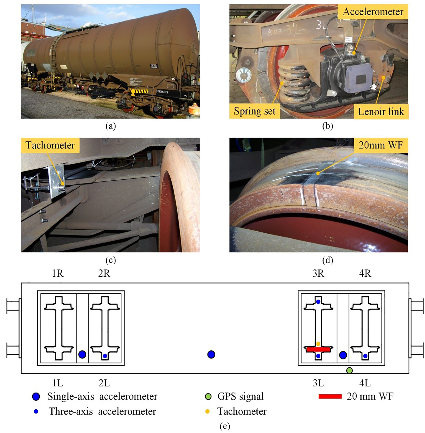
(a) Test wagon, (b) ABA measurement, (c) axle rotational speed measurement, (d) 20 mm WF,² and (e) measurement scheme.

Before starting the on-track experiment, a single WF with a length of 20 mm shown in Figure 1(d) was artifically produced on the wheel tread of the left wheel of the third wheelset (wheel 3L). Then the surface roughness was measured by using the wheel roughness measuring system from the company Ødegaard & Danneskiold-Samsøe A/S,²⁸ as presented in Figure 2(a). This system has three detectors and their measuring positions to the wheel flange are 65, 75, and 85 mm, respectively. The average measurement result is illustrated in Figure 2(b) and the flat depth is 0.32 mm.

Figure 2.

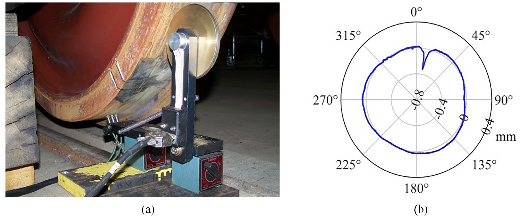
(a) Wheel roughness measurement and (b) measurement results.

The measurement scheme is illustrated in Figure 1(e). Four triaxial accelerometers were used to measure the accelerations of axle boxes (2L, 3L, 3R, 4L), while vertical accelerations of the front bogie, the rear bogie, and the car body were recorded by uniaxial accelerometers. Both two kinds of accelerometers have a sampling frequency of 5000 Hz. The accelerometer on the wheel 3L, as shown in Figure 1(b), is a Brüel & Kjaer Type 4520 triaxial piezoelectric accelerometer with a sensitivity of 1.02 mV/(m/s²), and its maximum measurement range is up to 1000 m/s².²⁹ The GPS device with a sampling rate of 1 Hz was used to measure the running speed of the wagon. As shown in Figure 1(c), a tachometer was installed on the bogie frame to record the number of revoluations of the third wheelset. The tachometer is a laser retro-reflective photoelectric sensor and it can read up to 1000 revolutions per minute, which corresponds to the wagon’s operating speed of 173 km/h. The running speed of the wagon in this research is below 100 km/h, and the tachometer can achieve precise measurements of the wheel’s rotational speed. Besides, the wagon was operated on the Ludwigshafen–Kaiserslautern railway line in Germany. More information about this experiment can be found in the study by Krause and Hecht.³⁰

Experimental results analysis

In this section, the influence of a single WF on accelerations of the axle box, bogie frame, and car body will be presented, including its influence on the left and right ABAs of the same wheelset, on ABAs of different wheelsets, and on vertical accelerations of the bogie and car body. All the data in this chapter is taken from the Kaiserslautern–Ludwigshafen journey, which is explained in detail in the section “Application II.” As introduced in the section “WF experiment introduction,” a single WF with a length of 20 mm is produced on the wheel 3L before the journey while the other wheels are intact.

ABAs of the same wheelset

Figure 3 presents ABAs of the third wheelset in three directions (longitudinal X, lateral Y, and vertical Z) when the running speeds are 20 and 80 km/h, respectively.

Figure 3.

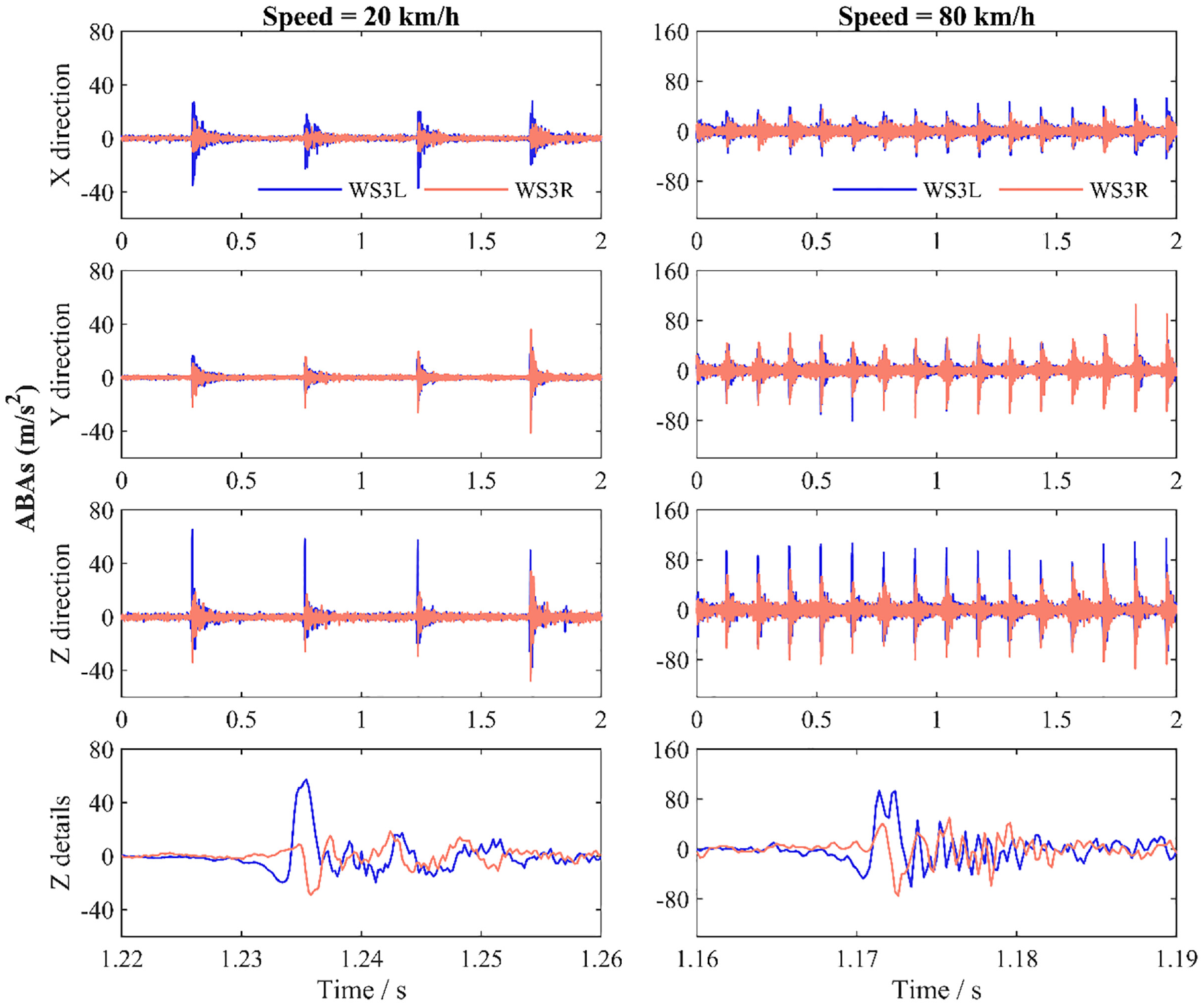
Comparison of ABAs of the same wheelset in the time domain when running speeds are 20 and 80 km/h (X/Y/Z: longitudinal/lateral/vertical directions) (WS3L: left wheel of the third wheelset).

Firstly, the single WF with a length of 20 mm on the left wheel (WS3L) can cause severe impact on ABAs in three directions, especially in the vertical direction. For instance, when the running speed is 20 km/h, the maximum accelerations of the WS3L in three directions (X/Y/Z) are 36, 24, and 65 m/s², respectively. Secondly, the impact occurring on the right wheel appears when the left wheel passes through the WF zone and therefore, a single WF on the left wheel can also induce the impact on the right wheel within the same wheelset. Thirdly, the running speed has a significant influence on the amplitude of impact accelerations, and impact peaks in the same direction when the running speed is 80 km/h are generally higher than those when the speed decreases to 20 km/h. For instance, all peaks of vertical ABAs of the WS3L are below 80 m/s² when the speed is 20 km/h, while most of the peaks are larger than 80 m/s² when the speed is increased to 80 km/h. At last, the vertical motions of the left and right wheels affected by the single WF are different. From 1.22 to 1.26 s, the vertical ABA of the left wheel will drop first and then has an impact peak when going through the WF zone at a speed of 20 km/h. However, the vertical ABA of the right wheel increases first and then drops sharply, which is caused by the roll motion of the wheelset. This phenomenon is also observed when the speed is increased to 80 km/h.

ABAs of different wheelsets

Figure 4 compares vertical ABAs of the left wheels of the second, third, and fourth wheelsets (WS2L, WS3L, WS4L) when the running speed is 20 and 80 km/h, respectively. When the wheel WS3L runs through the WF zone and induces an impact on the rail, small peaks can be observed on the wheel WS4L since it is close to the WF, and those peaks can be negligible compared to the peaks on the wheel WS3L. Besides, no significant peaks are observed on the wheel WS2L since it is far from the WF. In summary, a single WF has no important influence on the vibration of adjacent wheelsets due to the effect of suspension systems.

Figure 4.

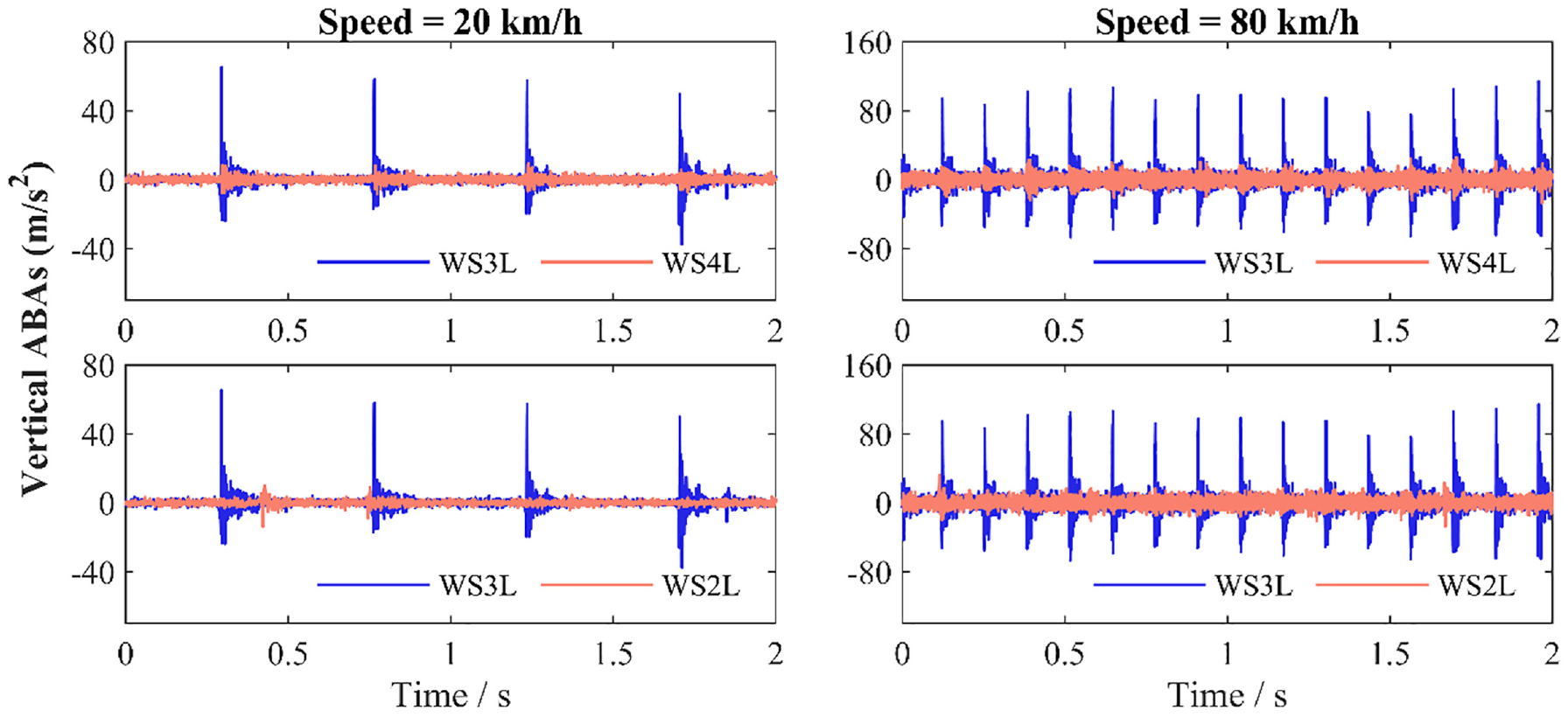
Comparison of vertical ABAs of different wheelsets in the time domain.

Vertical accelerations of axle box, bogie, and car body

Figure 5 illustrates vertical accelerations of the axle box of the wheel WS3L, the rear bogie frame, and the car body when the running speeds are 20 and 80 km/h, respectively. It can be seen that the WF can induce a significant impact on the vibration of the axle box and the bogie frame in the time domain while its influence on the vibration of the car body is not so apparent. The possible reason is that the measured point on the car body is on its center, which has a large spacing from the damaged wheel, and the impact energy caused by the WF is largely dissipated by suspension systems and the body structure.

Figure 5.

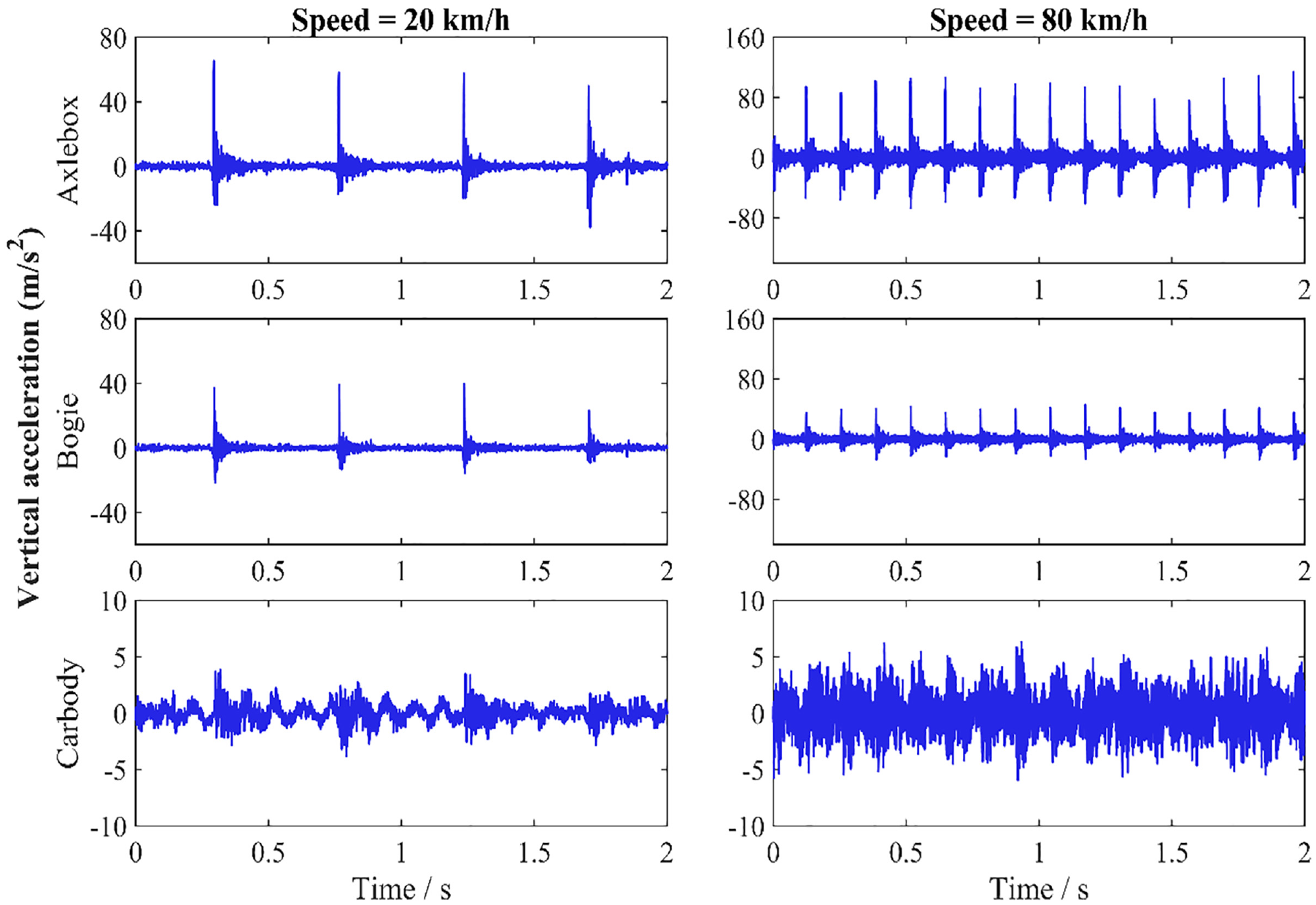
Comparison of vertical accelerations of the axle box, bogie, and car body in the time domain.

The corresponding response in the time-frequency domain during 0.2–0.8 s is presented in Figure 6, and it is calculated by continuous wavelet transform.^19,20 When the speed is 20 km/h, the main impact frequency on the axle box and the bogie frame is below 500 Hz. When the speed is increased to 80 km/h, impact frequency bands become much wider and some impact amplitudes on the axle box are up to 1500 Hz.

Figure 6.

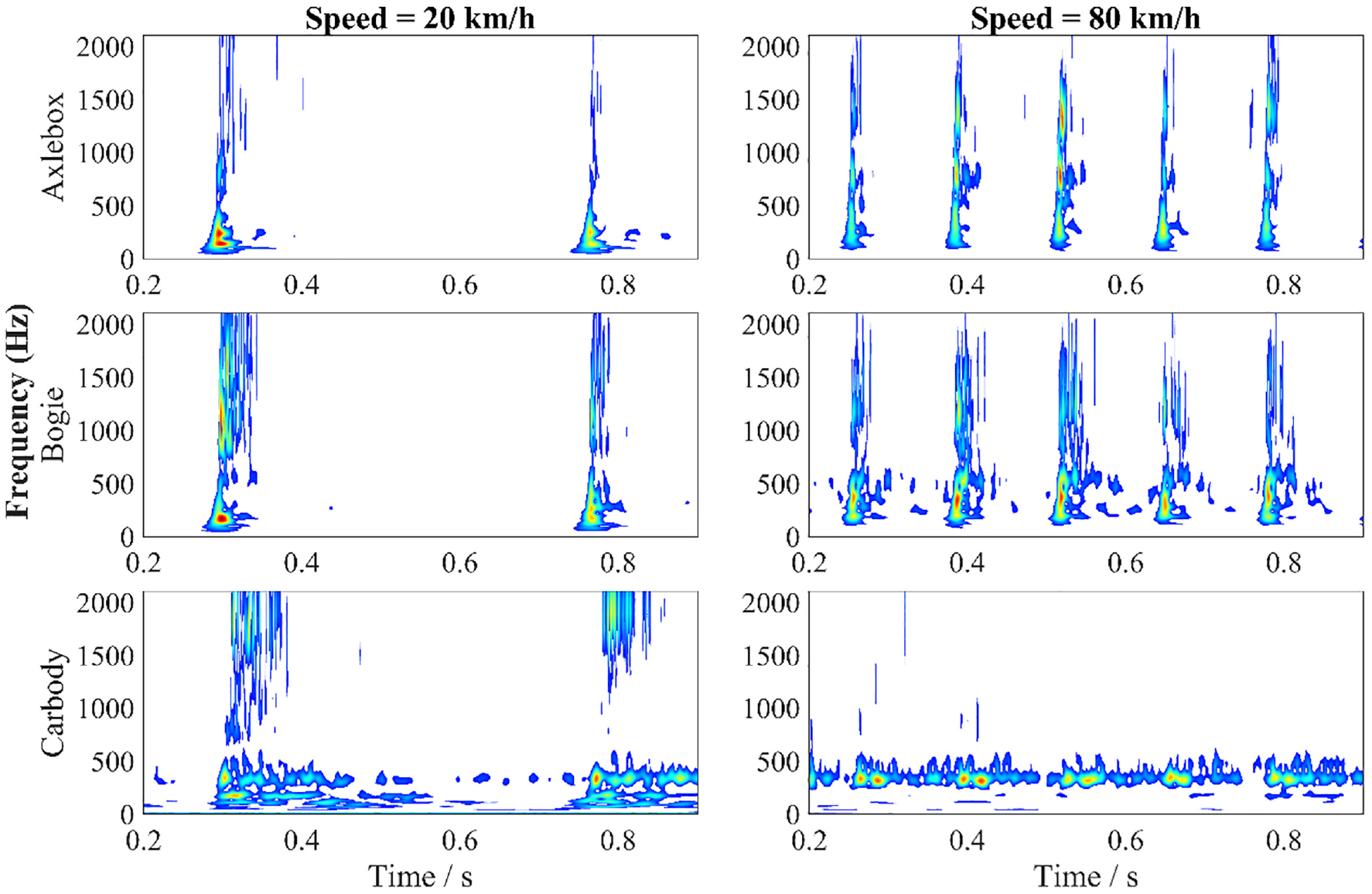
Comparison of vertical accelerations of the axle box, bogie, and car body in the time-frequency domain.

Vibration comparison of healthy and defective wheels

The combined influence of WF and the running speed on vertical accelerations of the axle box and bogie frame is shown in Figure 7. The ABA data of the defective wheel with a WF is measured on the wheel WS3L while that of the healthy wheel is obtained from the wheel WS2L. The defective and healthy bogie frame accelerations are obtained from the rear and front bogies, respectively. The data in 10 s is captured for each speed, and RMS values and peaks during this period are calculated. The acceleration signals of the axle box and the bogie frame both have a clear impact peak affected by the WF, and therefore the average of those peaks in 10 s is presented. Since healthy signals of the axle box and the bogie frame have no significant peaks, the 99th percentile of the data is regarded as the maximum value. The calculation details in 2 s for each speed are attached in Appendix 1.

Firstly, the ABA and bogie frame acceleration peaks of the defective wheel are much higher than those of the healthy wheel. For instance, when the running speed is 81 km/h, the ABA peak of the defective wheel is approximately eight times that of the healthy wheel while the maximum bogie frame acceleration is about seven times that of the healthy wheel. Although the maximum values of those accelerations have an increasing trend with the increase of the speed, the ratio of peaks has an opposite changing trend. Secondly, RMS values of the ABA and bogie frame acceleration of the defective wheel are more than two times that of the healthy wheel. For instance, when the speed is 81 km/h, the ratios are about 3.0 and 2.7 for the ABA and bogie frame acceleration, respectively. Although the statistical method is capable of detecting wheel defects, it is difficult to define a threshold to classify defective and healthy wheels. For example, the wheel can be classified as a defective wheel if the ratio of peaks is over this threshold. Since vibration signals are affected by the significance of wheel damage (WF length and depth), vehicle characteristics (load and suspension system) and track conditions (geometry and irregularities), the threshold is generally defined according to operating experience and data accumulation, which means that the threshold varies in different scenarios.

Figure 7.

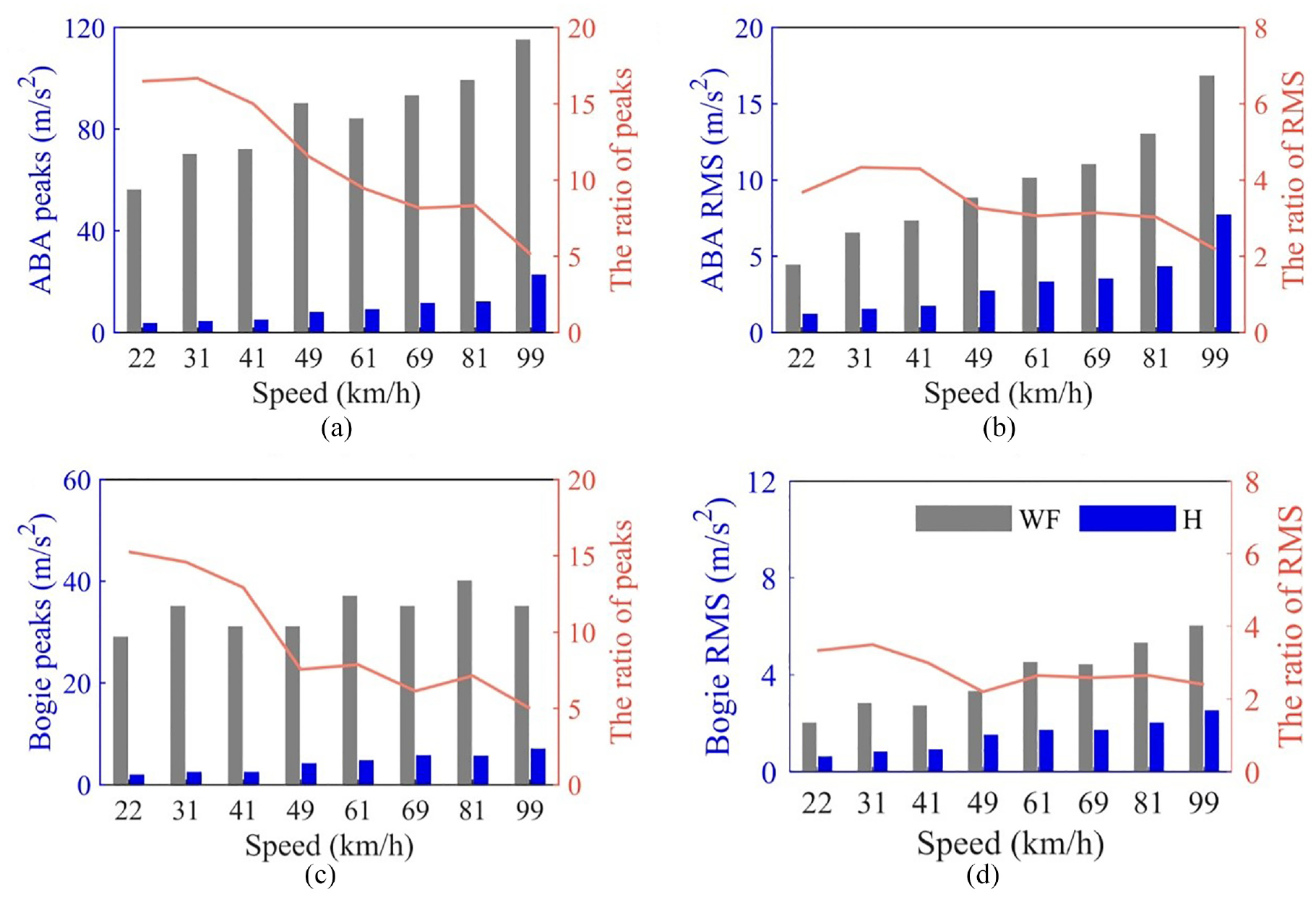
Combined influence of WF and running speed (H: healthy wheel).

ADSA method for WF detection

In this section, the theory of the ADSA method is first explained and then its effectiveness is compared with the envelope spectrum technology^16,17 in three scenarios.

ADSA method

Angle domain analysis is a technique for viewing data acquired from rotating machinery and it means that data is referenced to the angle of rotation rather than the time domain. Generally, we analyze vibration signals in the time domain, and the peaks caused by the WF get closer together as the speed increases over time. By transforming the same data from the time domain to the angular domain, the peaks are evenly spaced in the angular domain regardless of speed variations. The synchronous averaging technology can remove the noise or uncorrelated signals and retain the pulse signal or any signal correlated to the pulse signal.^31,32 Therefore, the ADSA method calculating the synchronous averaging vibration energy in the angular domain is used in this study to detect WFs, and the working flow of this method includes four steps, as shown in Figure 8.

Step 1: Measure the wheel rotational speed with tachometers and collect the ABA data using accelerometers.

Step 2: Transform the ABA data from the time domain to the angular domain based on the tachometer signal and extract the vibration vector of each wheel turn along the circumferential direction, denoted as ${\vec{X}}_{i}$ , where i represents the i th wheel turn. Note that the distance between one pulse of the tachometer and the next one represents one wheel turn, corresponding to 0–360° in the angular domain, and we assume the vehicle’s running speed is constant in one wheel turn.

Step 3: Calculate the average vibration energy of each wheel turn using the synchronous averaging technology. The ADSA is calculated by the equation

ADSA = \frac{1}{N} \overset{N}{\sum_{1}} {\vec{X}}_{i}

(1)

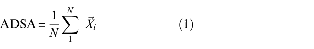
where N is the total wheel turns during a period. In the example presented in Figure 8, the ADSA is calculated when N is equal to 100. A clear “falling-rising-falling” process caused by the WF is observed on the ADSA curve, and the maximum amplitude is 20 m/s², which is generally lower than a single high peak but stronger than a single weak impact. Besides, the ADSA on the healthy circumferential position of this wheel, such as from 60 to 360°, is close to zero and it reveals that the ADSA of a healthy wheel is close to zero. For a long-distance journey, it is a good way to split the ABA data into several datasets by setting a constant time interval Δt. It has two advantages. On the one hand, we can find out in which time slot or track position the WFs occur, and track managers can also reschedule the maintenance plan since the wheel with WFs bumps the track periodically. On the other hand, it could improve the detection accuracy of WFs. For example, if a WF occurs on the last ten minutes of a 2-h journey and we use the ADSA method for the whole journey, the WF characteristics might not be reflected on the ADSA curve since the healthy signals account for a larger portion of the total signals.

Step 4: Describe the ADSA in the polar coordinate for a better display.

Figure 8.

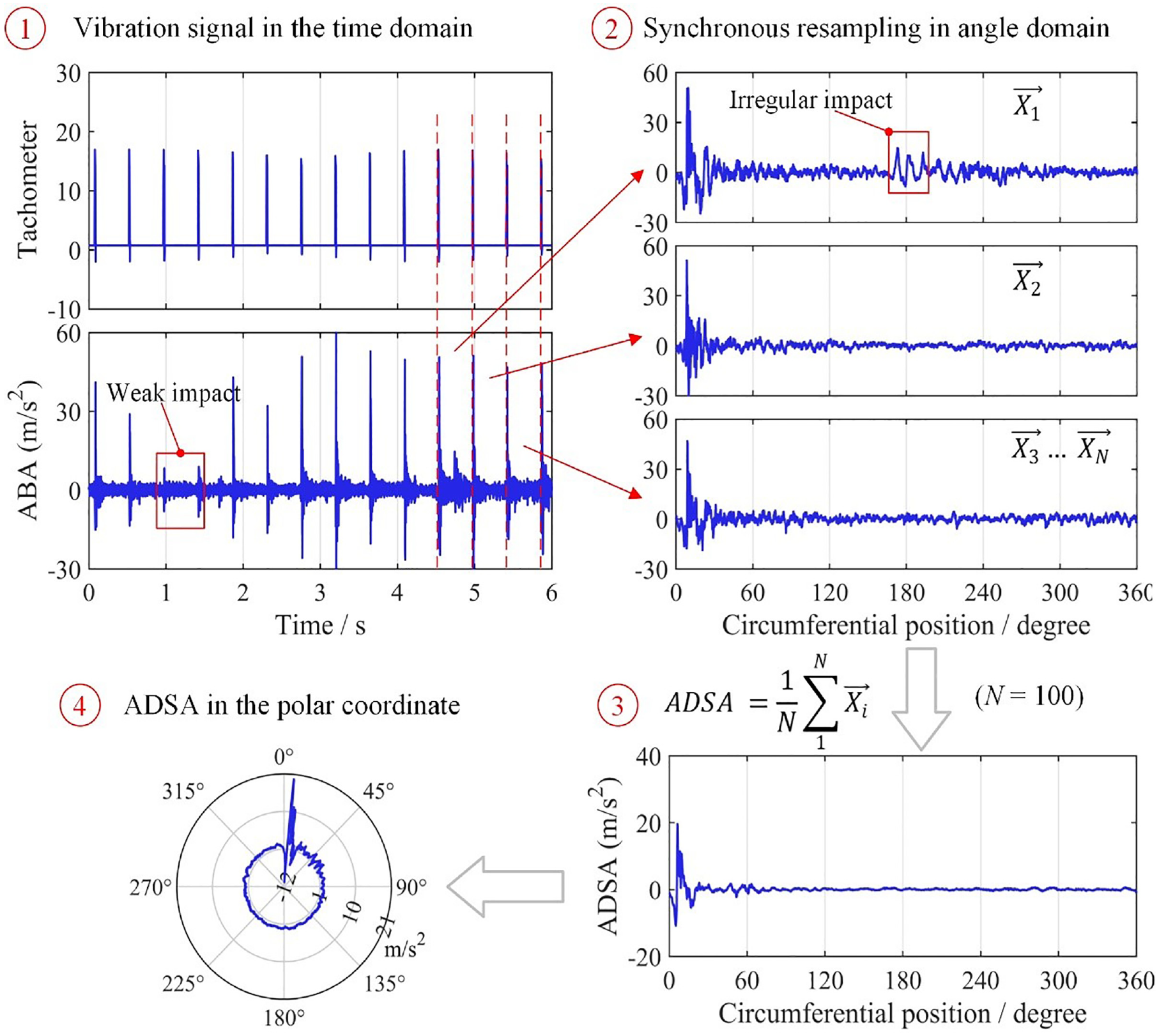
The ADSA method.

The first advantage of this method is that it can greatly compress the amount of measured data without losing the characteristics caused by the WF. For instance, if we measure vertical ABA with a sampling frequency of 5000 Hz for 2 h, we will get 5000 × 2 × 3600 = 36,000,000 data points. If we use the ADSA method and average the data every half hour with a sampling frequency of 0.1°, we only need 4 × 360 × 10 = 14,400 data points to represent the original data. Secondly, this method can remove the short-time influence of interference signals. On the one hand, some peaks caused by the special track geometry like switches and crossings or rail joints also can be measured besides peaks resulting from the WF. For instance, there is an irregular impact occurring around 180° of the first wheel turn, and it barely can be observed on the ADSA curve. On the other hand, some peaks caused by the WF might be not obvious due to the complex track geometry. All these short-time interferences can harm detecting wheel faults in the time domain. However, those influences will be largely weakened if adopting the ADSA method. Besides, this method is easily understood and implemented. The challenge is that the axle rotational speed information is also required besides the necessary vertical ABA data. It should be noted that the GPS signal is not accurate enough to get the axle rotational speed due to the low sampling rate, unpredictable wheel rolling diameter, and so on.

Comparison with envelope spectrum analysis

Case I: stationary vibration of a healthy wheel

Figure 9(a) illustrates the ABA signal of a healthy wheel for 30 s when the vehicle’s running speed is approximately 41 km/h. The axle rotational frequency f can be obtained

f = \frac{v / 3.6}{π d}

(2)

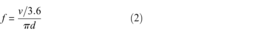
where v is the running speed (km/h) and d is the wheel diameter (m). The rotation frequency is 3.94 Hz when the nominal wheel diameter of 0.92 m is given. No obvious frequencies related to the wheel rotation frequency can be observed in Figure 9(b). However, the irregular impact on the wheel from the track structure has an influence on the envelope spectrum and it might affect the detection accuracy. The result of WF detection using the ADSA method is shown in Figure 9(c). No significant impulse can be observed and the average vibration energy fluctuates around zero, indicating that the wheel has no periodical defects. Compared to the envelope spectrum technology, the influence of track irregularities or defects can be better removed by using the ADSA method.

Figure 9.

Comparison of the envelope technology and the ADSA method for processing the stationary vibration of a healthy wheel (a) Vertical ABA and running speed, (b) Envelope analysis result and (c) ADSA result.

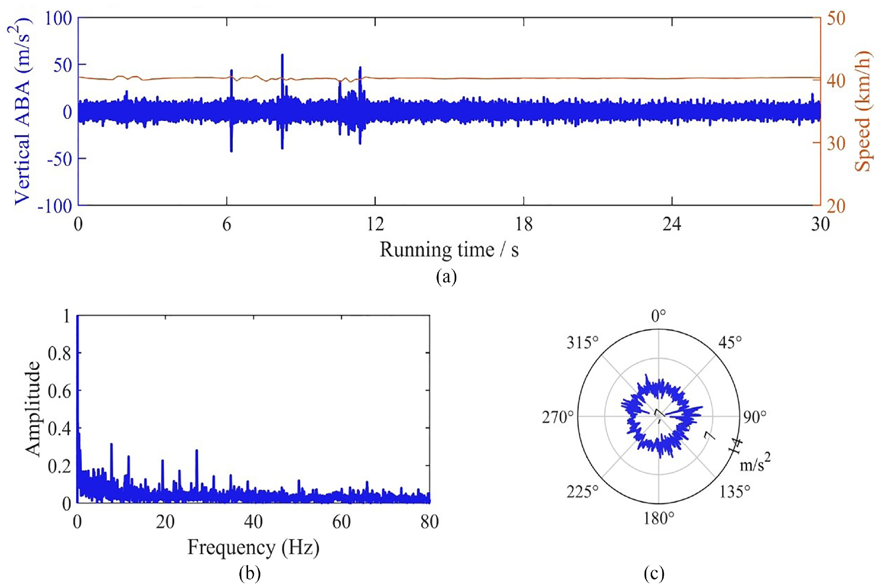
Case II: stationary vibration with WF signals

Figure 10(a) shows the ABA signal with the WF with a length of 20 mm when the vehicle’s running speed is approximately 81 km/h. The axle rotational frequency f is 7.69 Hz according to Equation (2). However, the real wheel diameter varies during operation since the wheel profile has a small slope, which causes the difference between the theoretical frequency of 7.69 Hz and the observed frequency of 7.65 Hz. Figure 10(b) reveals that a periodic impulse occurs in each wheel turn by using the envelope spectrum technology. The WF can also be detected by using the ADSA method. As illustrated in Figure 10(c), a clear “falling-rising-falling” process occurs at 0° of the polar coordinate, and the maximum value is 104 m/s². The number of WFs can be counted by both methods. Unlike envelope spectrum technology, the waveform caused by the WF can be displayed using the ADSA method.

Figure 10.

Comparison of the envelope technology and the ADSA method for processing the stationary vibration with WF signals (a) Vertical ABA and running speed, (b) Envelope analysis result and (c) ADSA result.

Case III: non-stationary vibration with WF signals

Figure 11(a) presents the ABA signal with the WF with a length of 20 mm when the vehicle’s running speed varies from 45 to 7 km/h. The axle rotational frequency f is changing from 4.32 to 0.67 Hz. A frequency of 2.43 Hz is observed on the envelope spectrum as shown in Figure 11(b), and it corresponds to the period between 28 and 54 s, which has a constant running speed of 25 km/h. The number of WFs is not able to be well detected in the whole scenario with time-varying speeds when using the envelope technology. However, the wheel defects can be well identified for the non-stationary vibration by using the ADSA method. As presented in Figure 11(c), a clear impulse caused by the WF appears at 0° of the polar coordinate, and the maximum value is 57 m/s².

Figure 11.

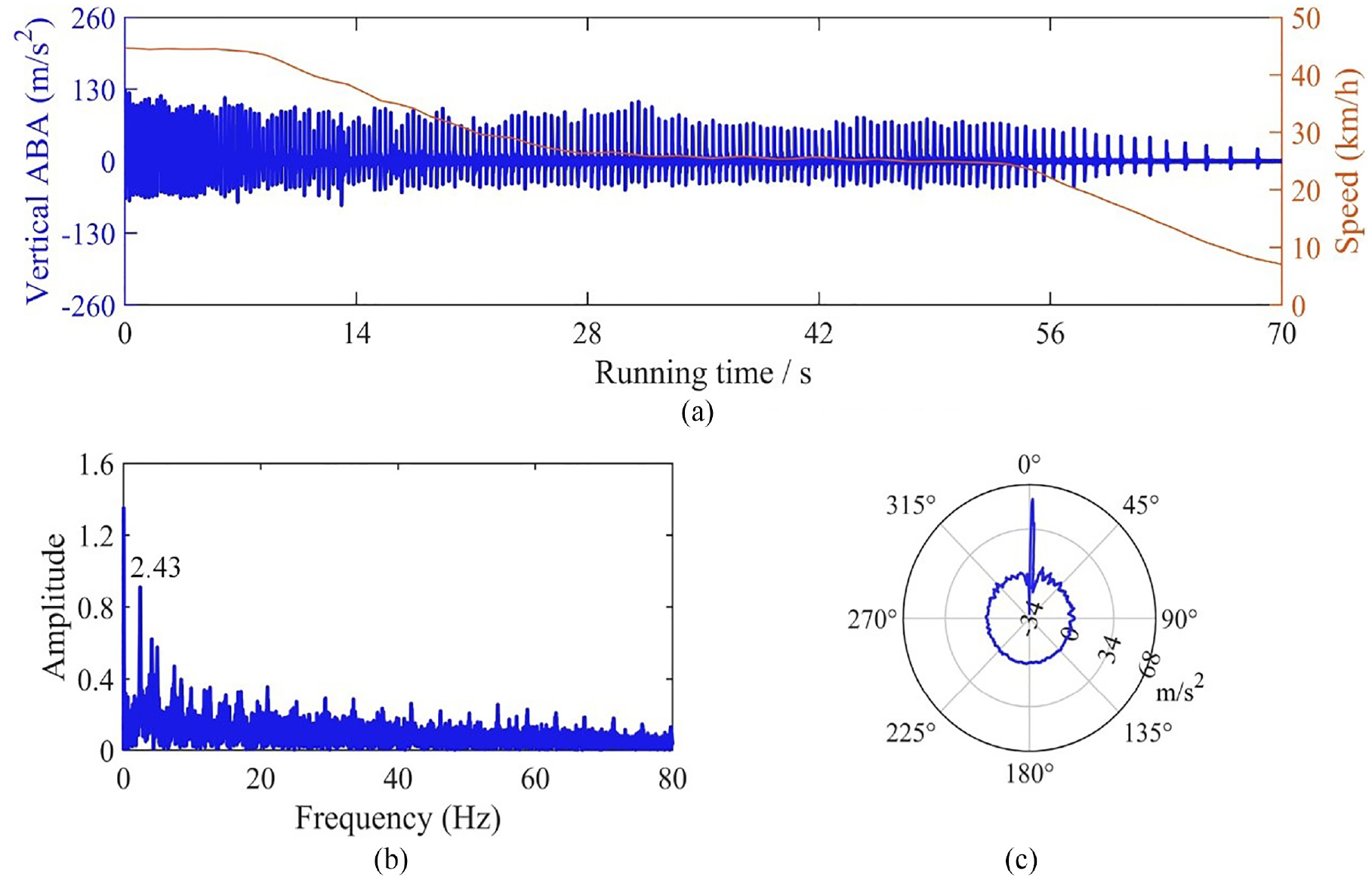
Comparison of the envelope technology and the ADSA method for processing the non-stationary vibration with WF signals (a) Vertical ABA and running speed, (b) Envelope analysis result and (c) ADSA result.

Application of the ADSA method

Three applications of the ADSA method are introduced in this chapter. One is the application of the ADSA method to a healthy wheel and the other two applications are the use of this method to detect the WF with a length of 20 mm in different journeys.

Application I

Figure 12 shows the speed information of the two-hour journey, which is a part of the journey from Ludwigshafen to Ruhland in Germany. The wagon’s speed varies from 0 to 100 km/h during this journey and all the wheels are intact. The speed calculated by the tachometer signal has a good agreement with that measured by the GPS device, which verifies the effectiveness of the tachometer signal.

Figure 12.

Running speed of the test wagon (Ludwigshafen–Ruhland).

The ADSA results of a healthy wheel during this journey are presented in Figure 13. In this work, a time interval of 0.5 h is taken and therefore the whole data is divided into four datasets. Besides calculating the averaging vibration energy at each point on the circumference, the distribution of the running speed during each period is also presented. Firstly, no significant impact can be observed on the ADSA curve, and the average vibration energy along the wheel circumferential orientation fluctuates around zero. Secondly, the maximum ADSA is pretty low compared to the case with the WF. For instance, the maximum ADSA values of a healthy wheel in three time slots are 2, 2, and 5 m/s², respectively. Since the wagon stops on the track for most of the third period, its ADSA result is not presented here.

Figure 13.

ADSA results of a healthy wheel without WFs (Ludwigshafen–Ruhland).

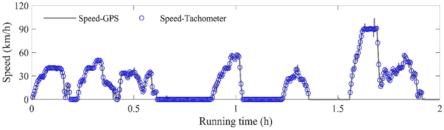
Application II

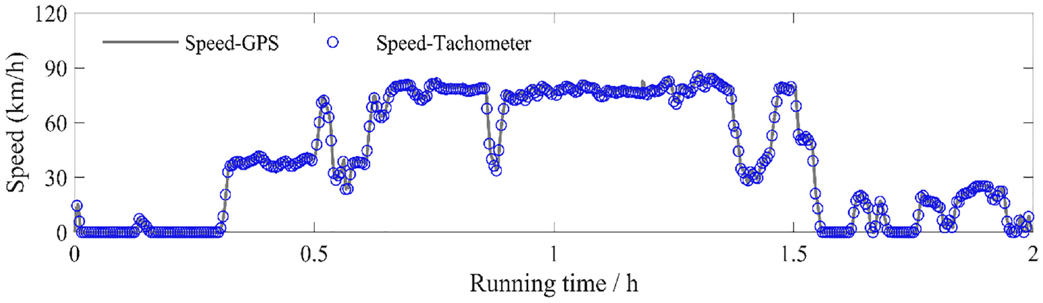
Figure 14 shows the speed information of the journey from Kaiserslautern to Ludwigshafen. The whole journey takes 2 h and the wagon’s speed varies from 0 to 100 km/h. The speed calculated by the tachometer signal is consistent with that measured by the GPS device.

Figure 14.

Running speed of the test wagon (Kaiserslautern–Ludwigshafen).

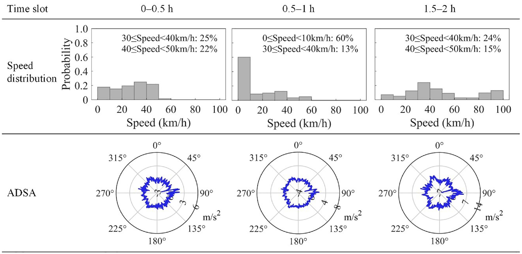
As introduced in the section “WF experiment introduction,” a single WF with a length of 20 mm was created on the wheel 3L before the start of this journey. The ABA data and the axle rotational speed of this wheel are measured, and the result of WF detection by using the ADSA method is presented in Figure 15. Since the wagon either stops on the track or runs at a low speed (20–30 km/h) during the first period, its ADSA result is not presented here.

Figure 15.

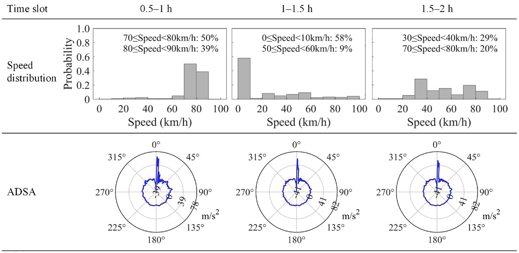
WF detection by using the ADSA method (Kaiserslautern–Ludwigshafen).

During the 0.5–1 h period, the vehicle mostly operates at speeds ranging from 70 to 90 km/h. A “falling-rising-falling” process is observed on the ADSA curve at around 0° in the polar coordinate and the maximum value is 63 m/s². It reveals that a periodical defect appears on the wheel and it is mostly like a WF according to the waveform of the defected signals. Once a WF appears, it can’t be removed automatically. Therefore, similar impulses are seen in the last two time slots as well. The maximum values are 60 and 55 m/s² for the time slots 1–1.5 and 1.5–2 h, respectively.

Application III

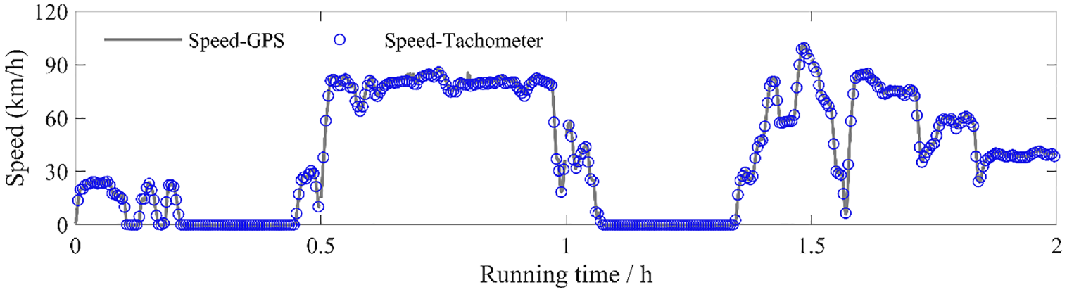
The running speed of the return journey from Ludwigshafen to Kaiserslautern is illustrated in Figure 16, and the travel time is approximately 2 h. During this journey, the running speed is below 90 km/h. The speed calculated by the tachometer signal also has a good agreement with that measured by the GPS device. Note that no wheel reprofiling is executed before the return journey, which means that the WF is still on the wheel 3L.

Figure 16.

Running speed of the test wagon (Ludwigshafen–Kaiserslautern).

The corresponding WF detection results during this journey are presented in Figure 17. Similar to application II, an abnormal peak occurs on the ADSA curve during each period, and it appears on the same wheel circumferential position, at around 8°. The maximum amplitudes in three time slots are 62, 52, and 21 m/s², respectively, and the results indicate that a periodic defect occurs on the wheel. Changes in the impact position between Application II and application III are caused by changes in the running direction of the wagon.

Figure 17.

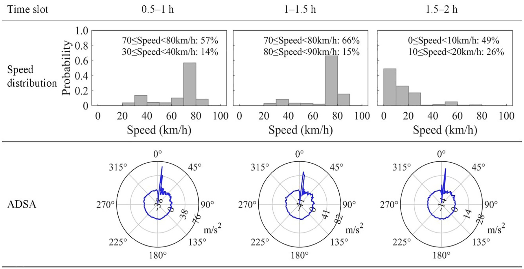
WF detection by using the ADSA method (Ludwigshafen–Kaiserslautern).

Conclusion

To study the dynamic impact caused by WFs, a single WF with a length of 20 mm was artifically produced on the wheel of a tank wagon. Its influence on the ABAs of the same and adjacent wheelsets, vertical accelerations of bogies and the car body is presented from an experimental perspective. The results show that the presence of WFs within the same wheelset has a significant effect on the ABA responses of that wheelset, and its effect on the ABA responses of adjacent wheelsets might be negligible. Secondly, the dynamic impact caused by a WF can also be well presented on the vertical acceleration signals of the bogie where the WF occurs, while its influence on the vertical acceleration of the car body is not so significant. Thirdly, the main impact frequencies on the axle box and the bogie frame are below 500 Hz in the low-speed range, and they become much wider when the running speed is increased. Besides, the peak ratio between defective and healthy ABA signals or bogie frame acceleration signals is more than 5 under various speeds while the ratio of corresponding RMS values exceeds 2. Although those statistical results might identify the defective wheel with WFs, it is difficult to define a specific threshold for different vehicles and different WFs in various running scenarios.

To better detect the defective wheel with WFs, the ADSA method is employed in this work and it requires vertical ABA data and the axle rotational speed as input. On the one hand, its effectiveness is compared with the envelope spectrum technology in three scenarios: stationary vibration of a healthy wheel, stationary, and non-stationary vibration with WF signals. On the other hand, three applications of the ADSA method are illustrated in this study. The first application demonstrates the use of the ADSA method on a healthy wheel while the remaining two applications illustrate the detection of the WF with a length of 20 mm for different journeys. The results show that this method can greatly reduce the amount of data by merging data into the angular domain and the ‘falling-rising-falling’ process on the ABA data caused by the WF can be well reflected in polar coordinates. Secondly, the ADSA method can remove the effect of speed variations and can be applied to non-stationary vibration processes, which is a great advantage over the envelope spectrum technology. Besides, this method is also easy to implement and understand. The ADSA of a healthy wheel fluctuates around zero in the polar coordinate while that of a defective wheel with a WF has a clear peak with an amplitude of 21–104 m/s², which is an indicator for distinguishing a defective wheel from healthy wheels. This method can be not only a near real-time detection method by setting a short time interval as presented in the section “Comparison with envelope spectrum analysis” but also a method processing the vibration data after the journey by setting a half hour time interval as introduced in the section “Application of the ADSA method.”

Note that all the vibration signals in this study were measured based on an artificial WF. The effectiveness of the ADSA method for detecting a natural WF should be further validated in future work, and its accuracy as a percentage should be given.

Footnotes

Appendix 1 Acknowledgements

The authors would like to thank all the colleagues from the Chair of Rail Vehicles at the Technische Universität Berlin who have participated in the field test, especially the project leader Philipp Krause and the technical assistant Dirk Itzeck.

Declaration of conflicting interests

The author(s) declared no potential conflicts of interest with respect to the research, authorship, and/or publication of this article.

Funding

The author(s) disclosed receipt of the following financial support for the research, authorship, and/or publication of this article: The first author is supported by China Scholarship Council (grant no.: 201907000128). The support is gratefully acknowledged.

ORCID iD

Yichang Zhou

References

Iwnicki

Spiryagin

Cole

, et al. Handbook of railway vehicle dynamics. London: Taylor & Francis, 2020.

Shi

Krause

, et al. A data-driven method for estimating wheel flat length. Veh Syst Dyn 2019; 58: 1329–1347.

Kumagai

Ishikawa

Haga

, et al. Factors of wheel flats occurrence and preventive measures. Wear 1991; 144: 277–287.

Wallentin

Bjarnehed

Lundén

Cracks around railway wheel flats exposed to rolling contact loads and residual stresses. Wear 2005; 258: 1319–1329.

Shi

Krause

, et al. Wheel flat can cause or exacerbate wheel polygonization. Veh Syst Dyn 2019; 58: 1575–1604.

Zhu

Huang

, et al. OORNet: A deep learning model for on-board condition monitoring and fault diagnosis of out-of-round wheels of high-speed trains. Measurement 2022; 199: 111268.

Zhang

Wei

Andrawes

, et al. Numerical and experimental study on dynamic behaviour of concrete sleeper track caused by Wheel Flat. Int J Rail Transp 2015; 4: 1–19.

Bian

Murray

MH.

A dynamic wheel–rail impact analysis of railway track under wheel flat by finite element analysis. Veh Syst Dyn 2013; 51: 784–797.

Yang

Boogaard

Chen

, et al. Numerical and experimental study of wheel-rail impact vibration and noise generated at an insulated rail joint. Int J Impact Eng 2018; 113: 29–39.

10.

Zhao

, et al. Effect of wheel flat on dynamic wheel-rail impact in railway turnouts. Veh Syst Dyn 2021; 60: 1829–1848.

11.

Thompson

DJ.

A hybrid model for the noise generation due to Railway Wheel Flats. J Sound Vib 2002; 251: 115–139.

12.

Yang

Thompson

DJ.

Time-domain prediction of impact noise from wheel flats based on measured profiles. J Sound Vib 2014; 333: 3981–3995.

13.

Alemi

Corman

Lodewijks

Condition monitoring approaches for the detection of railway wheel defects. Proc Inst Mech Eng Part F J Rail Rapid Transit 2016; 231: 961–981.

14.

Barke

Chiu

WK.

Structural health monitoring in the railway industry: a review. Struct Health Monit 2005; 4: 81–93.

15.

Brizuela

Fritsch

Ibáñez

Railway wheel-flat detection and measurement by ultrasound. Transp Res Part C Emerg Technol 2011; 19: 975–984.

16.

Mosleh

Montenegro

Costa

, et al. An approach for wheel flat detection of railway train wheels using envelope spectrum analysis. Struct Infrastruct Eng 2020; 17: 1710–1729.

17.

Nowakowski

Komorski

Szymański

, et al. Wheel-flat detection on trams using envelope analysis with Hilbert transform. Lat Am J Solids Struct 2019; 16: 1–16.

18.

Bernal

Spiryagin

Cole

Wheel flat detectability for Y25 railway freight wagon using vehicle component acceleration signals. Veh Syst Dyn 2019; 58: 1893–1913.

19.

Liang

Iwnicki

Zhao

, et al. Railway wheel-flat and rail surface defect modelling and analysis by time–frequency techniques. Veh Syst Dyn 2013; 51: 1403–1421.

20.

Jia

Dhanasekar

Detection of rail wheel flats using wavelet approaches. Struct Health Monit 2007; 6: 121–131.

21.

Belotti

Crenna

Michelini

, et al. Wheel-flat diagnostic tool via wavelet transform. Mech Syst Signal Process 2006; 20: 1953–1966.

22.

Bracciali

Cascini

Detection of corrugation and wheelflats of railway wheels using energy and Cepstrum analysis of rail acceleration. Proc Inst Mech Eng, Part F J Rail Rapid Transit 1997; 211: 109–116.

23.

Chen

Wang

Chang

, et al. A two-level adaptive chirp mode decomposition method for the railway wheel flat detection under variable-speed conditions. J Sound Vibr 2021; 498: 115963.

24.

Shi

Gillwald

, et al. Designing a lightweight 1d convolutional neural network with bayesian optimization for wheel flat detection using carbody accelerations. Int J Rail Transp 2020; 9: 311–341.

25.

Shi

Gillwald

, et al. Robustness enhancement of machine fault diagnostic models for railway applications through data augmentation. Mech Syst Signal Process 2022; 164: 108217.

26.

Iwnicki

Stichel

Orlova

, et al. Dynamics of railway freight vehicles. Veh Syst Dyn 2015; 53: 995–1033.

27.

Zhou

Hecht

Running safety analysis of a freight train passing through a single crossover during braking. Veh Syst Dyn 2021; 60: 3519–3539.

28.

Johansson

Andersson

Out-of-round railway wheels—a study of wheel polygonalization through simulation of three-dimensional wheel–rail interaction and wear. Veh Syst Dyn 2005; 43: 539–559.

29.

https://www.bksv.com/de/transducers/vibration/accelerometers/ccld-iepe/4520.

30.

Krause

Hecht

Energieautarke Sensorsysteme zur Zustandsüberwachung am Güterwagen. ZEVrail 2017; 141: 116–124.

31.

Sun

Chen

Kemp

, et al. An on-board detection framework for polygon wear of railway wheel based on vibration acceleration of axle-box. Mech Syst Signal Process 2021; 153: 107540.

32.

Zhang

Tang

Integrating angle-frequency domain synchronous averaging technique with feature extraction for Gear Fault Diagnosis. Mech Syst Signal Process 2018; 99: 711–729.

Wheel flat detection on railway vehicles using the angular domain synchronous averaging method: an experimental study

Abstract

Keywords

Introduction

WF experiment introduction

Experimental results analysis

ABAs of the same wheelset

ABAs of different wheelsets

Vertical accelerations of axle box, bogie, and car body

Vibration comparison of healthy and defective wheels

ADSA method for WF detection

ADSA method

Comparison with envelope spectrum analysis

Case I: stationary vibration of a healthy wheel

Case II: stationary vibration with WF signals

Case III: non-stationary vibration with WF signals

Application of the ADSA method

Application I

Application II

Application III

Conclusion

Footnotes

Appendix 1

Acknowledgements

Declaration of conflicting interests

Funding

ORCID iD

References