
Abstract
A large quantity of civil infrastructure in North America is near the end of their design life. Consequently, the routine visual structural inspection is increasingly necessary to ensure the safety and efficient management of the infrastructure stock. The increasing need for inspections and the laborious nature of the work has caused strain on the inspection industry. To improve inspection efficacy, various researchers have proposed novel deep learning methodologies to automatically classify, detect, and segment structural defects from images. After the defects are identified, it is often desirable to quantify the size of the defect, for severity classification and repair cost estimation. Yet, the measurement from a single image for quantification is not a trivial task, requiring supplementary data or sensor inputs, which may not be practical or economical in the current inspection process. In this study, we propose to recover the three-dimensional geometry of a scene from a single image, by using deep learning-based monocular depth estimation. The monocular depth estimation field has made great progress by leveraging deep learning and a plethora of open red, green, blue, and depth (RGB-D) datasets. However, there has not been a publicly available in situ Light Detection and Ranging (LiDAR) RGB-D dataset for the civil engineering domain, which is a barrier for researchers to develop and evaluate spatial computer vision methods in the civil engineering context. To bridge this gap, we build a LiDAR-based RGB-D dataset for training monocular depth estimators. Then using the civil RGB-D dataset, we test a solution for the real-world application of monocular depth estimation to quantify defects in civil infrastructure.
Introduction
In North America, a large quantity of infrastructure was built in the mid-20th century and has reached the end of its design life. Presently, the deterioration of infrastructure is outpacing our ability to replace them. This has greatly increased the need for routine inspections to monitor the condition of the infrastructure to inform maintenance schedules and replacement decisions. The most common inspection method employed is the visual inspection since external changes in the appearance of a structure can often be a good indicator of structural deterioration. By exploiting recent developments in computer vision and deep learning, numerous researchers have sought to automate visual inspection, which can improve inspection outcomes and reduce costs. 1
A typical visual inspection involves inspectors studying the visual appearance of the infrastructure. The inspectors then note any defects and if applicable make measurements or visual estimates of the defect for records and repair estimates. Researchers have proposed classification algorithms to identify defects in an image.2–7 To localize the defects in images, researchers have proposed various detection algorithms.8–11 To quantify the precise dimension of defects in images (e.g., crack length/width), researchers have proposed various semantic segmentation algorithms.12–16
Automated visual inspection methods typically quantify defects in image coordinates (i.e., pixels). Converting defect measurement from pixels to actual (metric) units is challenging, since the inverse projection from image to world requires a scale prior (i.e., depth). The most direct way to get depth information is to utilize specialized depth sensors such as stereo cameras, Light Detection and Ranging (LiDAR), laser scanners, and so on. 17 However, depth sensors are often expensive and may not always be available or practical. A popular alternative to depth sensors is by leveraging correspondences between multiple images using structure from motion (SfM). 18 SfM is a very popular method for large-scale civil survey and asset inspection (i.e., building façade, bridges, and dams), typically paired with unmanned aerial vehicles (UAVs) for data collection. 19 Then using the UAV’s inertial measurement units and real-time kinematic global positioning system, it’s possible calculate scale information to transform the SfM reconstruction to real scales. Thus, provided an image and depths from SfM reconstruction, it’s possible to quantify various defects.19–23 However, in practice, depth sensors and UAV-based SfM reconstructions are often not practical or economical for many inspections such as short-medium span overpass bridges.
Currently, the Ministry of Transportation Ontario (MTO) in Canada requires inspectors to capture an image of each defect. 24 In order to include a scale prior in the defect image, it is common for inspectors to include a known-size (reference) object (i.e., pen, notebook, ruler, etc.) near or co-planer to the defect. 7 The reference object method allows inspector to quickly collect data in the field, which reduces costs incurred due to traffic disruptions and the inspector’s time in field. However, the reference object method can be ergonomically challenging when the defect is large (i.e., it is challenging to fit a large spalling in camera frame while holding a measuring stick to the structure) and requires inspectors to manually inspect each image to find the appropriate pixel-to-metric scaling factor. Thus, it is desirable to infer metric depth from a single image, without reference objects, which can be directly utilized to quantify defects, similar to depths from sensors or UAV SfM reconstructions.
A promising field of research which attempts to infer depth from single images is monocular depth estimation, which learns depth cues such as known objects, vanishing lines, textures, and so on to regress depth. Numerous studies have shown that given an image, a deep monocular depth estimation model can produce a depth map of the scene, like that from a depth sensor. In contrast to the reference object method, monocular depth estimation for defect quantification can significantly reduce data collection effort, costs and eliminate the variability from estimating the sizes of defects.
Developments in monocular depth estimation methods are enabled by the availability of abundant red, green, blue, and depth (RGB-D) datasets, where in addition to the red-green-blue channel of a color image, there is a depth channel, such that the intensity of the pixel indicates the distance between the imaged scene and the camera center. RGB-D data are valuable for civil inspection, for example, to quantify structural deformations. 25 Additionally, RGB-D data have been shown to benefit semantic defect detection research through RGB-D fusion convolutional neural networks (CNNs). 26 However, RGB-D dataset in the civil domain is rare, as a result researchers are commonly forced to use RGB-D datasets from adjacent domains or create an ad-hoc depth data standard which may not be applicable to other works.26–28 Currently, to the best knowledge of the authors, there is no LiDAR RGB-D dataset of in situ civil infrastructure scenes, 29 which have significantly limited researchers’ ability to benchmark deep monocular depth estimation methods for the civil domain.27,28
The purpose of this work is to evaluate the real-world application of monocular depth estimation for defect quantification on civil infrastructure, enabled by a novel LiDAR civil RGB-D dataset. First, a custom scanner is created, which is used to efficiently collect civil RGB-D dataset of five railway overpass bridges, with distinct construction styles. Second, the scan data are processed to produce densified RGB-D frames through scan accumulation. This is accomplished by utilizing local poses generated from simultaneous localization and mapping (SLAM) and a depth buffer. Finally, the collected civil RGB-D frames are used to evaluate the applicability of popular monocular depth estimation methods for monocular defect quantification. Due to large variety of civil infrastructures and challenges to collect additional civil RGB-D data, model generlizability is proposed as an important performance indicator. The monocular depth estimation methods used in this work are evaluated on an unseen bridge, in zero-shot and few-shot configurations; their effect on model performance and spalling defect quantification accuracy are used as a case study.
The main contribution of this work is the development of an in situ LiDAR civil RGB-D dataset, which we use to fine-tune monocular metric depth estimation methods for the civil domain, specifically for the objective to measure structural defects from single images. Our study finds a direct correlation between quantification accuracy and the fidelity of depth estimation, which implies that depth estimation performance metrics may be used as proxy to compare models’ defect quantification accuracy. However, due to the high cost of collecting civil RGB-D data, depth estimation models with high generalizability are necessary to enable monocular defect quantification. In this study, we find that pre-tuned vision transformer monocular depth estimation models greatly outperformed fully convolutional neural network-based methods, potentially indicating an efficient path to create robust monocular defect quantification and other civil applications of monocular depth estimation.
Method overview
The objective of the monocular defect quantification method is to enable quantitative visual inspections only from a single image, without relying on extra sensor data. The basic premise is that provided an image with sufficient contextual information, a deep learning method can be trained to estimate the three-dimensional (3D) geometry of the scene. Then, given the defect locations on the image, its measurement can be obtained from that estimated 3D geometry. The benefit of this method is allowing the real size of the defect to be rapidly and directly estimated from a single image, such that the proposed method can readily be incorporated with existing vision-based semantic visual inspection algorithms, with the goal of a fully automated quantitative structural defect inspection procedure.
Figure 1 presents an overview of the proposed monocular defect quantification methodology. As a preliminary step, it is necessary to calibrate the camera used to collect inspection images (RGB). Camera calibration ensures the images from the camera are minimally distorted and allows the calculation of the camera intrinsic matrix (
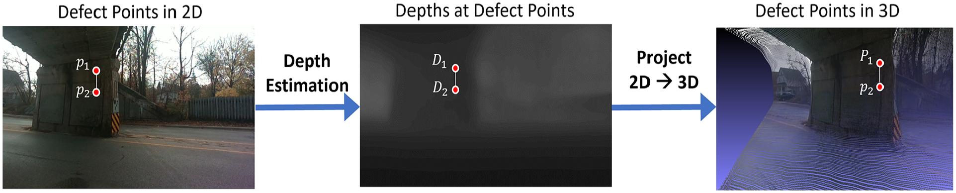
3D defect measurement through monocular depth estimation. 3D: three-dimensional.
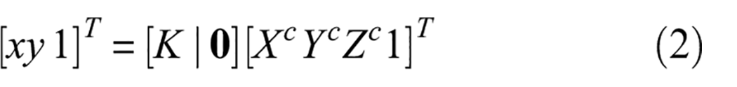
For actual measurement, the pixel coordinates selected are reprojected in 3D via a pinhole camera geometry. In Equation (7), the 3D coordinate can be computed by premultiplying its homogenous pixel coordinate vector (
The ability to recover the 3D information at each pixel can be used to obtain the quantification of the defect. As a potential application, inspectors quantify spalling using extreme points (i.e., maximum length and width), inspired by bridge inspection manual, Ontario Structural Inspection Manual (OSIM) pages 1–2–6, utilized by MTO. Inspectors manually select pairs of extreme points of a defect from the RGB image, projected at the points in 3D, and return their Euclidean distance. 24 The severity of the defect is classified based on these dimensions. Multiple defects can be measured if they are present in the same image. 24 Using the precomputed depth image, additional measurements can be made at low marginal computational cost. Thus, in addition to the maximum dimension required by OSIM, the users can also calculate a defect’s shorter dimension (i.e., secondary dimension), which is useful to estimate repair cost, shown in “Experiment” section.
Related work
The critical component of the proposed methodology involves utilizing monocular depth estimation, which estimates depth from a single two-dimensional (2D) image. While it is well understood that binocular vision enables depth perception, humans still navigate their surroundings, though at a reduced capacity using one eye. The widely accepted explanation is that humans can learn visual cues that provide insight about the depth of the scene. Many researchers have attempted to tackle monocular depth estimation and often to different ends. This typically impacts what “depth” means, such as relative (i.e., relatively consistent depths but not up to scale such as from SfM), ordinal (i.e., foreground verse background), or metric (i.e., meters). Since the proposed application in this study is to estimate the real size of the defect; thus, only metric depth estimation methods are reviewed.
The monocular depth estimation field took off after the introduction of deep CNNs. Eigen et al utilized a coarse-to-fine scale CNN network, trained with a scale-invariant loss. 32 Li et al. attempted to improve the pixel-level depth estimation through local feature similarity by first estimating super-pixel level, then pixel-level surface normal and depths, which are postprocessed with conditional random fields (CRFs). 33 Xu et al. utilized CRFs to integrate multiple-scale intermittent depths during depth up-sampling. 34 CRFs are a great way to enforce consistency and continuity in-depth predictions. Laina et al. proposed utilizing convolutional residual networks (i.e., ResNets) instead of AlexNet-inspired architecture first proposed by Eigen et al.35,36 The residual connections allowed the implementation of deeper networks and make the residual network able to learn depth up-sampling without CRFs for postprocessing. 35 Recently, deep residual networks have become the de facto standard for monocular depth estimation, with many researchers proposing incremental improvements. Fu et al. proposed to re-pose depth regression as an ordinal classification. 37 Yin et al. incorporated geometric constraints through an additional loss term that penalized the difference in the normal between some randomly chosen three points. 38 Lee et al. proposed a local planar guidance (LPG) layer module, which helps up-sampling encoded features with local planer assumption. 39
Most recently, transformer models, like many other computer vision tasks, have also begun to proliferate the monocular depth estimation studies.40–42 Transformer models have many advantages over deep CNNs mainly being able to learn long-range dependencies (i.e., global receptive field) through tokenization and attention mechanism, and a greater capacity to encode large amounts of data. 43 Where previously, CNN researchers proposed changes to models’ architectures, Ranftl et al. proposed a data-centric perspective for monocular depth estimation. 40 Such that instead of training and testing on a single dataset, Ranftl et al. set state-of-the-art benchmarks by training with various public RGB-D datasets (up to 12). To accomplish this, they first normalized depths of datasets and used a multiobjective loss function, which is necessary to overcome loss instability due to differences in the depths between datasets. 40 A limitation of the method is that at inference their model can only output relative depth maps, which have limited utility. Recently, Bhat et al. extended the work by Ranftl et al., by only training with relative depth datasets, with a metric-bin decoder which allows the fine-tuning to a metric depth dataset. 42
A challenge with using larger models with an increased number of parameters is the risk of overfitting. In the context of a vision model, a sufficiently large model can “memorize” the instances in the training set. Overfitting can result in poor model performance on unseen data as it is said that the model fails to generalize to the data. The ability of a model to generalize, known as “genralizability,” is important to its real-world applicability of monocular depth estimation in the civil domain, due to the sometimes bespoke nature of civil infrastructure and the high cost to collect additional data. For example, structural designs depend on local demand, collecting spatial data requires mobilization of sensors to site and site conditions may require additional safety and regulatory considerations. Consequently, the lack of civil RGB-D datasets has necessitated civil researchers in depth estimation to study more constrained problems and utilize smaller models.27,28
Conventionally, in defect detection (i.e., defect detection and segmentation), researchers fine-tune a large model by fixing early parameters and allowing latter parameters to be changed from the fine-tuning dataset. However, the conventional ideas of fine-tuning are not applicable to metric monocular depth estimation. 44 This is because metric depth values can depend heavily on the camera parameters and differences in distributions of depths between datasets can create unstable losses, which are detrimental to model training. 42
We recognize that the civil RGB-D dataset presented in this study is relatively small and limited in its range, particularly when compared to more established RGB-D benchmarks. Gathering a comprehensive RGB-D dataset for civil structure is inherently challenging due to the vast scale of structures and their restricted accessibility. This limitation could cause the risk of overfitting, especially when employing large, state-of-the-art transformer-based models for monocular depth estimation. Therefore, for domain-specific tasks, it may be more suitable to train a smaller, CNN-based model for monocular depth estimation. However, Bhat et al. have recently suggested the feasibility of “fine-tuning” a model designed for relative depth estimation to perform metric depth estimation. 42
Thus, in this work, the proposed civil RGB-D dataset is used to compare the model and generalizability performance between a representative CNN model and “Zero-shot Transfer by Combining Relative and Metric Depth: ZoeDepth” (ZOE), proposed by Bhat et al.. As a representative CNN-based monocular depth estimation model, we select “Big to Small: Multi-scale Local Planar Guidance for Monocular Depth Estimation,” proposed by Lee et al., popularly known as Big To Small (BTS). BTS is a great choice for learning monocular depth due to its strong performance on key benchmarks and ease of training due to its lightweight model. Additionally, BTS is uniquely suitable for civil applications due to its LPG module, which is a compatible inductive bias that can aid it the prediction of large planar surfaces, common of civil structures. In contrast, ZOE does not make any depth consistency assumption and requires much greater computational power to train and inference, yet, as it is able to leverage a much greater corpus of training data, it should exhibit greater model generalization than BTS. Thus, ZOE can exhibit greater model generalization than representative CNN methods, which have profound positive impact on real-world applicability of monocular depth estimation such as monocular defect quantification.
BTS uses a typical encoder–decoder architecture, where a CNN is used for feature extraction, and squeezed features are recovered using atrous spatial pyramid pooling and residual connections from the CNN encoder. At various stages of the decoder (scale), the up-sampled feature maps are used to predict depths via the LPG module. 39 The purpose of the LPG module is to convert the intermittent decoder features at each scale to the full input resolution, by explicitly regressing the four-dimensional plane coefficients at each pixel. The LPG module can better regularize depth predictions, with fewer learned parameters, which may be beneficial to model generalization. Finally, the full-resolution depth maps at each scale are concatenated, and a final convolutional layer is used to output the final depth prediction. 39
In contrast, ZOE utilizes a transformer encoder-decoder architecture as proposed by Ranftl et al., followed by their proposed metric depth learning module (metric bins). 42 The metric bins module utilizes multiscale features from the decoder and a multilayered perceptron (MLP) at each scale to predict which discrete depth range (depth bin) each pixel belongs. Such that for each pixel its coarse depth is the center of the depth range or depth bin center. To refine the depth prediction, Bhat et al. adjust bin center predictions with attractor points using another MLP along the depth interval. Finally, the adjusted depth bin centers are linearly combined by their probabilities, calculated using the log of the binomial probability predicted for each bin center. The metric bins module essentially poses depth estimation as a scale and shift problem, assuming the model has a good relative depth prediction. This allows ZOE to learn the meta scale and shift parameters of a particular dataset, and thus avoiding the potentially unstable losses during fine-tuning using metric depth data. Such that ZOE can leverage greater spatial understanding, gained from pretraining on a large corpus of diverse RGB-D datasets. In effect, a relatively small metric dataset can be used to fine-tune ZOE for a domain specific monocular metric depth estimation application.
RGB-D data collection
Hardware selection
Civil engineers inspect a wide variety of structures including bridges, culverts, dams, buildings, parking garages, and so on. We consider a hardware solution that may be practical for collecting spatial data in a wide range of inspectable structures. For example, the spatial sensor should be able to function both indoor, when inspecting from within, and outdoor, when inspecting from the exterior of a structure. Where indoor may have low-light and feature-scarce scenes, and inspecting from a structure’s exterior can present issues about access, which necessitates greater sensor range. Lastly, the sensor be economical and easy to utilize for rapidly generate RGB-D frames from multiple perspectives.
Among the many considered spatial sensing paradigms, such as structured light, stereo camera, SfM, and time-of-flight sensors, it was found that time-of-flight sensors are most able to meet the requirements outlined previously. For example, structure light sensors are not suitable for outdoor use, while stereo cameras and SfM rely heavily on image features, which may be unreliable for civil scenes.18,45,46 Additionally, there are two popular types of time-of-flight sensors: mobile LiDAR and static terrestrial laser scanners. 29 Terrestrial laser scanners are highly accurate and have a long sensing range; however, they are expensive and unsuitable to rapidly scan structures with complex geometries, due to the time-consuming task of relocating the scanner to obtain optimal coverage and diverse perspectives to create an RGB-D dataset for training.47,48 In contrast, mobile LiDAR is lower cost and can rapidly collect spatial data from the perspectives of the inspector, which makes it most suitable for creating an RGB-D dataset.49,50 With these considerations, we build a custom mobile LiDAR scanner to collect the RGB-D data from real-world structures.
Mobile scanning system
An objective of this work is to reduce the barrier for researchers to replicate the hardware and contribute their own scan data. To this end, only commercially available sensor and hardware are used, the spatial sensors used in this work the Livox Avia LiDAR and Intel Realsense D455 camera, shown in Figure 2. The Intel Realsense camera is mounted on top of the Livox Avia LiDAR, using a custom 3D printed bracket, additionally a bottom plate is attached below the LiDAR with a standard camera mount thread, allowing the sensor to be easily adaptable to different platforms. Figure 2 shows the scanner in a handheld and backpack configuration, which is ideal for the scanning of short-medium span overpass bridges, like those in “Experiment” section.
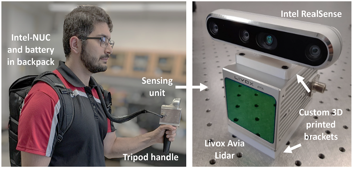
User carrying LiDAR scanner in backpack format (top). Custom-built handheld scanner equipped with Intel Realsense D455 camera and the Livox Avia for collecting dense depth images (bottom).
The Intel Realsense D455 camera is a highly modular, economical, robotic operating system compatible, computer vision camera.
51
The Intel Realsense’s RGB camera is capable of capturing images with a resolution of
To collect the depth data, the Livox Avia LiDAR sensor was used. The Livox Avia, like other LiDARs (e.g., Ouster Lidars), have a range of 3–200 m with an average depth measurement error of 1–2 cm. 52 Differently from rotating LiDARs, the Livox Avia is a semisolid-state LiDAR with a 70° field-of-view and scans in a nonrepeating rosette pattern. The nonrepeating rosette scanning pattern of the Livox Avia scans more points in the camera’s field-of-view, comparable to much more expensive spinning LiDARs. The high overlap between the camera and LiDAR field-of-view greatly aids in creating denser depth images after postprocessing in “Postprocessing” section.
For the camera and LiDAR to work as a unit, they need to have extrinsic calibration. In this work, extrinsic calibration was done after affixing the camera to the LiDAR using a custom 3D printed bracket, which bolts to existing mounting points on the LiDAR and camera housings. This allows the extrinsic calibrations to be embodied in the 3D printed mount, and thus researchers can directly 3D print and connect camera and LiDAR without additional calibrations steps. 53 Finally, the sensors were plugged into an Intel NUC mobile computer for collecting and storing data. In the backpack configuration as seen in Figure 2, the NUC, batteries, and miscellaneous hardware components are stowed in the backpack with a single wiring loom going over the user’s right shoulder, allowing for single-handed operation of the scanner. This setup enables a single operator to collect high-density RGB-D data of many types of civil infrastructure, for training monocular depth estimation in the civil domain.
Postprocessing
A challenge of integrating camera and time-of-flight sensors is that cameras take a near instantaneous snapshot of a scene, while LiDARs continuously send and evaluate the time to return of each laser. Where camera sensor’s resolutions are measured in millions of pixels a LiDAR sensor’s speed is measured in hundreds of thousand points per second. Thus, the disparity between LiDAR’s sampling rate and pixels per image results in very high sparsity in a depth image, which is unusable for deep learning tasks since sparse depth maps make inefficient supervision targets, resulting in poor training outcomes. To address this, issue depth accumulation was used, where a stream of LiDAR scan points is gathered to render a depth image corresponding to an RGB image. 54
Since the pose of the sensor also changes between sequential LiDAR scans, it is necessary to determine the relative poses of the sensor at each scan. To obtain the relative pose of the sensor, an open-source SLAM algorithm called R3LIVE was employed, which leverages the LiDAR scans, images, and IMU measurements to create a point cloud in the map frame. 55 A big problem with SLAM methods is drift, where small errors are compounded over time resulting in an incorrect odometry and point cloud map. 55 A popular way to mitigate drift is using loop-closure, where the user revisits a scanned location (e.g., the starting point), then the difference between relocalization pose and odometry are resolved using pose-graph optimization. 56 However, relocalization in civil environments is challenging and closing loops during inspection may not be practical (e.g., crossing the street). 57 Thus, to mitigate risk of drift, only the most recent LiDAR scans are considered to render the depth map, which assumes that local relative poses are relatively accurate. 54 In practice, the local point cloud map is a queue of some fixed size, where new points displace the longest existing points in the queue. In this work, the latest 250,000 points from the latest scans prior to a RGB image’s timestamp are stored, this is referred to as depth accumulation. This ensures that there are minimal errors between the local LiDAR point cloud and camera poses due to drift. Finally, the resulting accumulated LiDAR point cloud is projected onto the image plane of the RGB camera, assuming the pinhole camera model, using the camera pose estimated from SLAM. Figure 3 shows a visual representation of the accumulated LiDAR point cloud being projected on to an image frame.
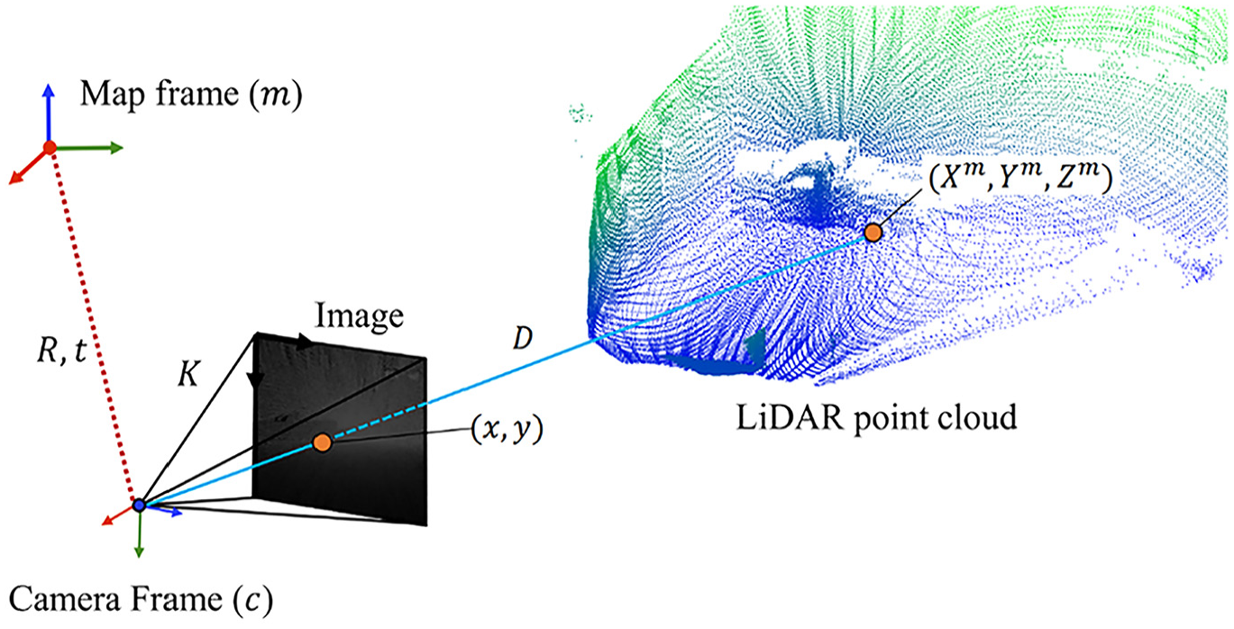
Depth image rendering from accumulated LiDAR point cloud using the pinhole camera model.
To render a depth image, we try to find the shortest length of a ray (
First, the accumulated point cloud needs to be transformed from the map frame to the camera frame. This transformation requires the extrinsic parameters, composed of the
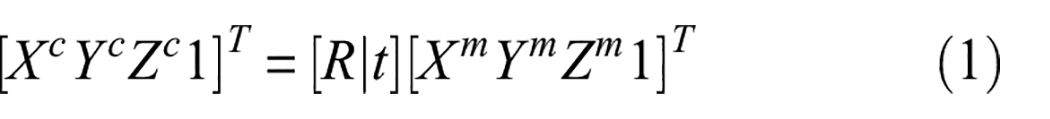
The transformation in Equation (1) ensures that the XY-plane is parallel to the image plane and thus the Z component represents the depth in the image. Thus,
Second, it is necessary to project each point in the camera frame to the image plane, per the pinhole (projective) camera model to obtain its depth. This projection requires
For each 3D point, the resulting x and y coordinates in the image plane were then rounded to the nearest integer such that each depth value is assigned to a specific pixel coordinate in the image.
Lastly, since the mapping between the set of 3D points in the camera frame to image pixel coordinates is not bijective, it can create an ambiguity about the depth in the depth image. For example, multiple 3D points could be projected to one pixel point. This is typically caused by occlusions due to ego-motion of the sensor. Then to resolve the correct depth image, we employed the depth buffer algorithm to guarantee that when multiple 3D points project onto the same image pixel, the one with the smallest depth value gets displayed. 58 This approach prioritizes selecting 3D points closer to the camera over those further away when producing the depth image.
This three-step process is repeated for each image with estimated pose from SLAM, which generates a dense depth image for each RGB image. We note that there are many configurations for postprocessing, such as number of accumulated points, points from past and future scans, image size, which can affect the density of the depth image and computational effort to render. These specific configurations will depend on the user’s application and thus we will provide the raw scan data, and the postprocessing scripts, along with this dataset.
For training monocular depth estimation in this work, images from the Intel Realsense are downscaled by a factor of 0.6, yielding a resolution of
Experiment
Bridge RGB-D datasets
The custom mobile scanning hardware was used to collect the data from five in-service bridges near downtown Kitchener, Ontario, Canada. These bridges support an elevated railway running East-West, crossing over Belmont St., Iron Horse Trail, Park St., King St., and Weber St. shown in Figure 4 (The order of the photos is from top to bottom and from left to right). These bridges are labeled as B1-B5.
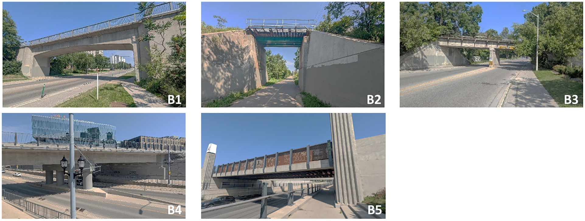
Five bridges utilized to construct the RGB-D dataset for this study.
The data collection took place from pedestrian-accessible paths and crossings surrounding each bridge. An effort was made to point the scanner to the bridge and to avoid scanning areas less than the minimum range of the LiDAR sensor (3 m). The sensor was held in front of the user at chest height, typically pointed in the direction of travel, the user can pitch the sensor, at the elbow, to ensure coverage of the bridge soffit. Images were collected at 30 Hz for the duration of each scanning session, which ranged from 3 to 7 min to scan a single bridge. In total, approximately 40,500 RGB-D frames were processed from all five bridges (B1: 7,294 frames, B2: 4,169 frames, B3: 7,024, B4: 10,523 frames, B5: 11,474 frames).
Figure 5 shows a sample RGB-D frames that include color and depth images. Where the lighter intensity pixels denote closer objects and vice versa, and the gray regions are pixels without depth data. The circular pattern of depth points results from the scanning pattern of the Livox Avia LiDAR, which utilizes a nonrepeating rosette pattern. Due to a small difference in the field of view between the Livox Avia LiDAR, 70° and the Intel Realsense D455, 90° there may be a lack of depth values at the border of the depth image (left and right of the depth image). This is most apparent when the sensor is stationary and is less apparent as the user moves and rotates the scanner to scan the structure.
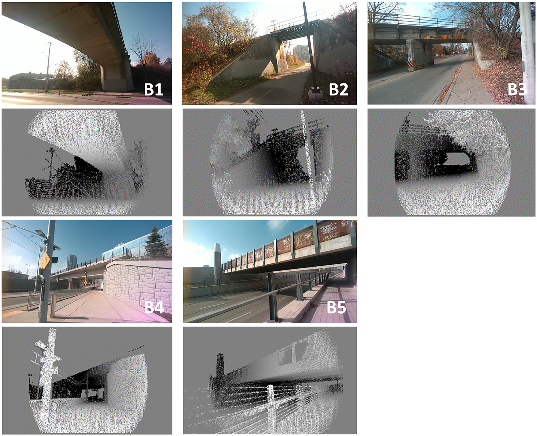
Sample RGB-D frames (RGB and depth images).
Due to the high sampling rate of the scanning system, the collected RGB-D frames may contain a significant number of redundant frames, such as subsequent frames with substantial overlap. Redundant frames do not significantly improve the accuracy of the depth estimation model and only increase the training time. 40 To address this issue, the frames from each bridge are down-sampled based on the location of the frame estimated from SLAM. Thus, to prepare the dataset, only those frames, where the relative displacement exceeded 10 cm from a previously chosen frame, were selected. Consequently, 7748 RGB-D bridge frames were selected to use for model development, in “Model development” section.
Model development
After postprocessing in “Post processing” section, the RGB-D images of
Key parameters for model training.
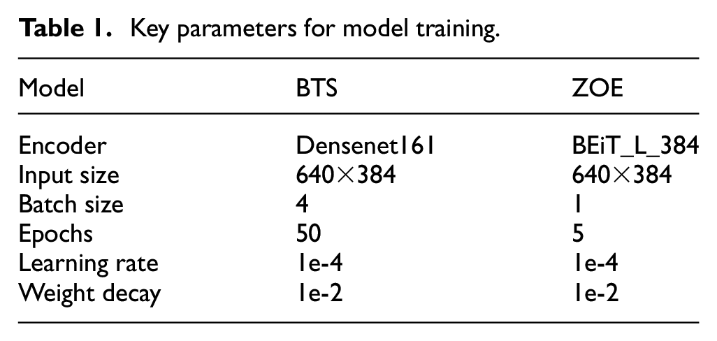
The models were evaluated using standard depth estimation metrics that have been recommended in various previous studies: average Absolute Relative error (AbsRel) in Equation (3), root mean square error (RMSE) in Equation (4), average log10 error (Log10) in Equation (5), and delta under thresholds (%) in Equation (6) 39 :
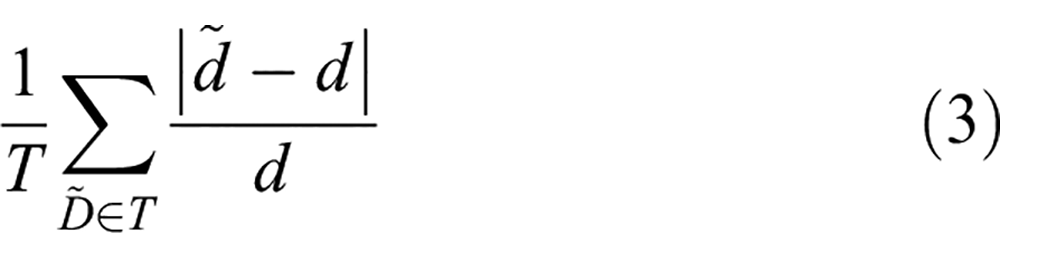
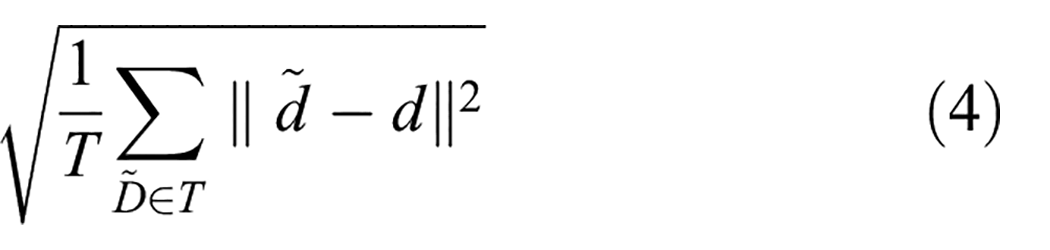
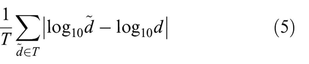
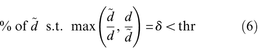
Here,
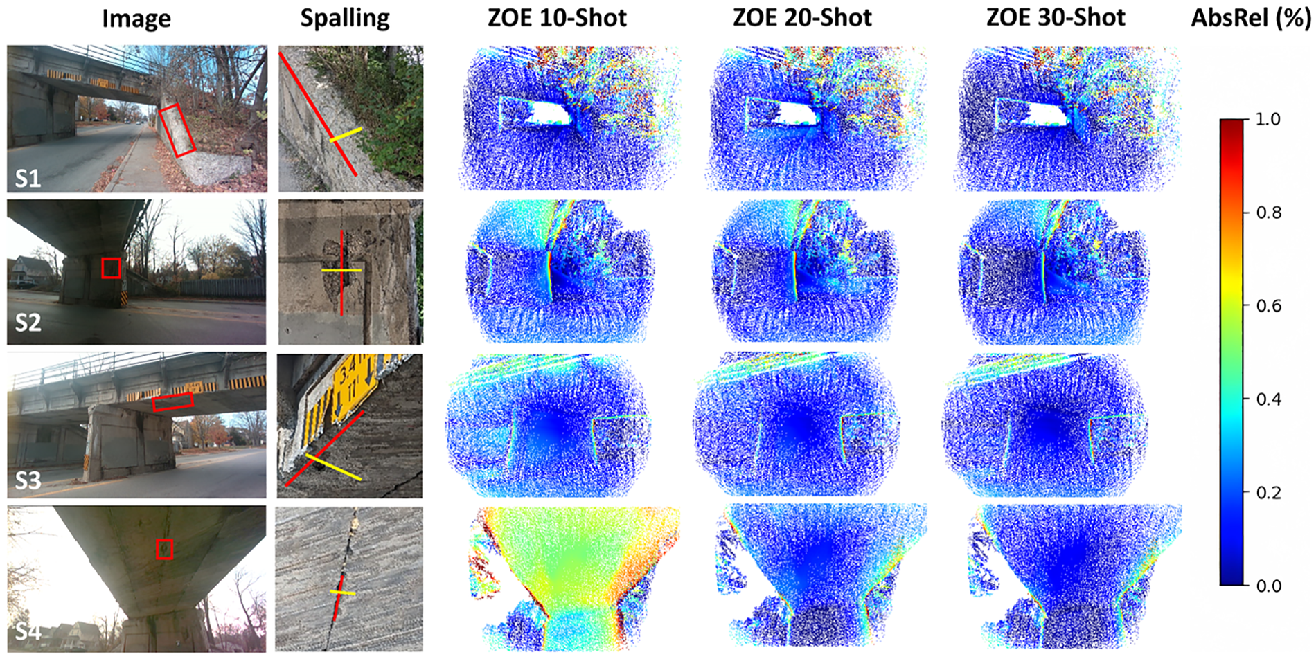
Comparison of AbsRel heatmaps for four spalling defects on bridge B3 using few-shot ZOE models.
Model generalizability
The main challenge with the bridge RGB-D dataset is that there are relatively few sequences and they are visually and structurally distinct. This must be expected because infrastructure is typically built to site requirements, and additional bridge RGB-D data are expensive and logistically challenging to obtain. Therefore, it is advantageous for a monocular depth model to learn robust depth cues that are relevant across various types of infrastructure. Essentially, the ability of the model to generalize is a crucial factor for its practical effectiveness in the real-world application of monocular defect quantification.
To evaluate the generalizability of BTS and ZOE in the civil domain, we test depth estimation performance in “zero-shot” and “few-shot” configurations using bridge RGB-D dataset. In the zero-shot configuration training was done (B1, B2, B4, and B5) sequences and inference on an unseen (B3) testing sequence. This is done to showcase the capacity of the model to learn robust depth cues for adapting to new scenes. With the zero-shot performance as a baseline, a smaller number of samples (10, 20, and 30 RGB-D frames) from the testing set (B3) into the training process, which is termed to “few-shot” in this work. The underlying idea is that the few-shot performance can further demonstrate the depth estimation capabilities of the model, by extrapolating from few testing samples (approximately 0.5, 1, and 1.5% of the B3 sequence), mixed into the training set, to infer the remainder of the testing sequence. This can simulate the effect of training with a more comprehensive bridge RGB-D dataset and provide insights about the applicability of monocular depth estimation models to inspections of more regular infrastructure (e.g., highway overpass bridge, parking garages).
Table 2 shows the model performance evaluation using the metrics shown in Equations (3)–(6) for BTS and ZOE in zero-shot, 10-shot, 20-shot, and 30-shot configurations. From Table 2, it is clear that ZOE greatly outperforms BTS model by demonstrating superior generalizability between the training sequences and testing sequence (zero-shot) and ability to generalize to the testing sequence with few samples (few-shot). Comparing the zero-shot performance, ZOE demonstrates a 4% reduction (i.e., approximately 20% improvement) in AbsRel error and a 13% increase in percentage under the 25% threshold. Similarly, with the few-shot models, ZOE is observed to perform significantly better than BTS. For example, from Table 2, ZOE 10-shot outperforms BTS 30-shot, and the ZOE 30-shot model nearly halves the AbsRel and Log10 error compared to the BTS 30-shot model. This can also be observed in the performance improvement between zero-shot and 30-shot performance, for example, the AbsRel error of BTS showed a 35.7% improvement, while ZOE showed a 52.3% improvement, between zero-shot and 30-shot. These findings indicate that ZOE is much more efficient and applicable for learning robust depth cues in civil engineering settings, like bridges, which are diverse in construction and have a high cost for data collection. This indicates that ZOE-like methods could be valuable in developing monocular depth estimation applications, such as defect quantification, within the civil engineering domain.
Evaluation of the model performance using various metrics in Equations (4)–(6).
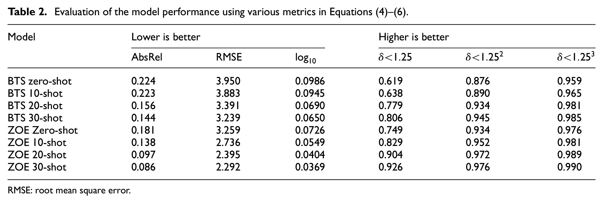
RMSE: root mean square error.
Defect quantification
The testing bridge B3 is a concrete slab bridge, with a center pier, built in 1931. A major issue for B3 is spalling of concrete on the abutment wall, central pier, and soffit. Spalling defects have the potential to expose underlying steel reinforcement in the structure, which results in accelerated structural degradation. Inspectors typically use a ruler to measures the length and width of the spalling defect, where the maximum length or width is used to severity, and the total area is used to create repair estimates. 24 However, this manual method can be complex and costly, in this case requiring traffic control and elevating equipment for inspectors to safely access and evaluate the damage. In contrast, we utilize monocular depth estimation to quantify spalling defects, from single images taken from the sidewalk.
From a preliminary walk-through, four spalling defects were identified in bridge B3, labeled S1-S4, as depicted in Figure 6. In order to find a relationship between model performance and spalling quantification accuracy, the ZOE few-shot models are used. Pairs of 2D points on the testing images, corresponding to the largest primary and secondary dimension of the spalling, corresponding to its length and width, are manually selected from images. Such that the same 2D points are projected into 3D using ground-truth and predicted depth images, to ensure consistency. The largest dimension is marked as the primary (in red), and the smaller as the secondary (in yellow). Then, these points’ pixel coordinates are converted into 3D coordinates in metric units using the inverse projection formula described in Equation (7). In Equation (7),
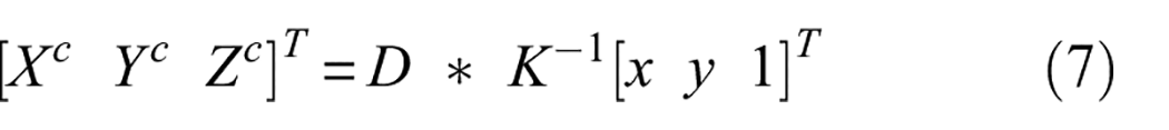
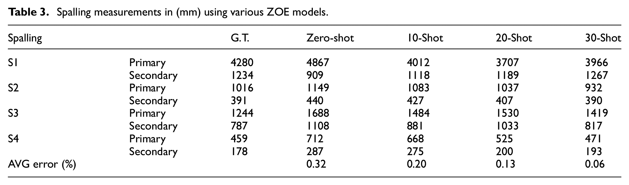
Table 3 reports the measurements of S1–S4 using ZOE models described in the preceding section. Differently from the global depth metrics in Table 2, each defect measurement is the result of sampling two pixel values in the depth prediction, which can sometimes result in outlying defect measurement results. However, on average measurement accuracy of ZOE zero-shot, 10-shot, 20-shot, and 30-shot models are 32, 20, 13, and 6%, respectively. We believe these results can be meaningfully improved with further research, as encouragingly even with 10 testing samples, at 20% average measurement error, the ZOE model can provide a rough estimate of the size of spalling damage, which may be useful with quantized damage severity and estimation methods. For example, OSIM classifies spalling severity in four categories by their maximum measurement: light (less than 150 mm), medium (between 150 and 300 mm), severe (between 300 and 600 mm), and very severe (more than 600 mm). 24 Moreover, for spalling repair estimates, it is common for the defect area to be rounded up to a convenient dimension (e.g., the nearest half meter (500 mm)), since loose concrete around the spalling may need to be chipped prior to the repair. 59
Spalling measurements in (mm) using various ZOE models.
To further understand the potential cause of measurement errors, the AbsRel heatmaps are plotted, which provide the per-pixel absolute percentage difference between the ground-truth depth and depth predictions in Figure 6. Where regions of low AbsRel error is shown in dark blue and clipped at a maximum AbsRel error of 100% in red.
The average defect measurement error is roughly correlated with the AbsRel metric of the model in Table 3. This indicates that a model’s performance can be used as a proxy for the quantification accuracy. However, it is also observed, from Figure 6, that depth prediction errors are not equally distributed. Where the sidewalk, roadway, bridge slab, and pier are generally well estimated, there are some error prone regions for example, at sharp depth transitions (i.e., bridge soffit to sky, bridge pier to abutment, and vegetation) and the bridge soffit. Particularly, the models have difficulty to inference the correct angle between the bridge soffit and pier, such that if the soffit and pier are not perfectly square, the greater the error in the soffit as it diverges from the ground-truth, as seen in the scene S2 and S4, in Figure 6. The spatial context of the bridge soffit is challenging to learn since images of the soffit typically contain fewer depth cues, and this difference can be observed when comparing the predictions between spalling S3 and S4, from Figure 6. Where spalling S3, near the side of the soffit, is more accurately measured compared to spalling S4 in the middle of the soffit. Encouragingly, S4 appears to be learnable; however, requiring additional samples compared to S1, S2, and S3.
Lastly, we utilized the ZOE models to measure the same spalling defects, S1–S4, from images collected with a personal smartphone, since they are commonly used by inspectors to collect images of defects. In this experiment, a Google Pixel 6a was used; however, any modern device may be utilized, as long the camera intrinsic can be obtained from its manufacturer. To control for metric depth ambiguity caused by difference in focal lengths, the cellular images have been scale- and crop-augmented such that the transformed image intrinsic (
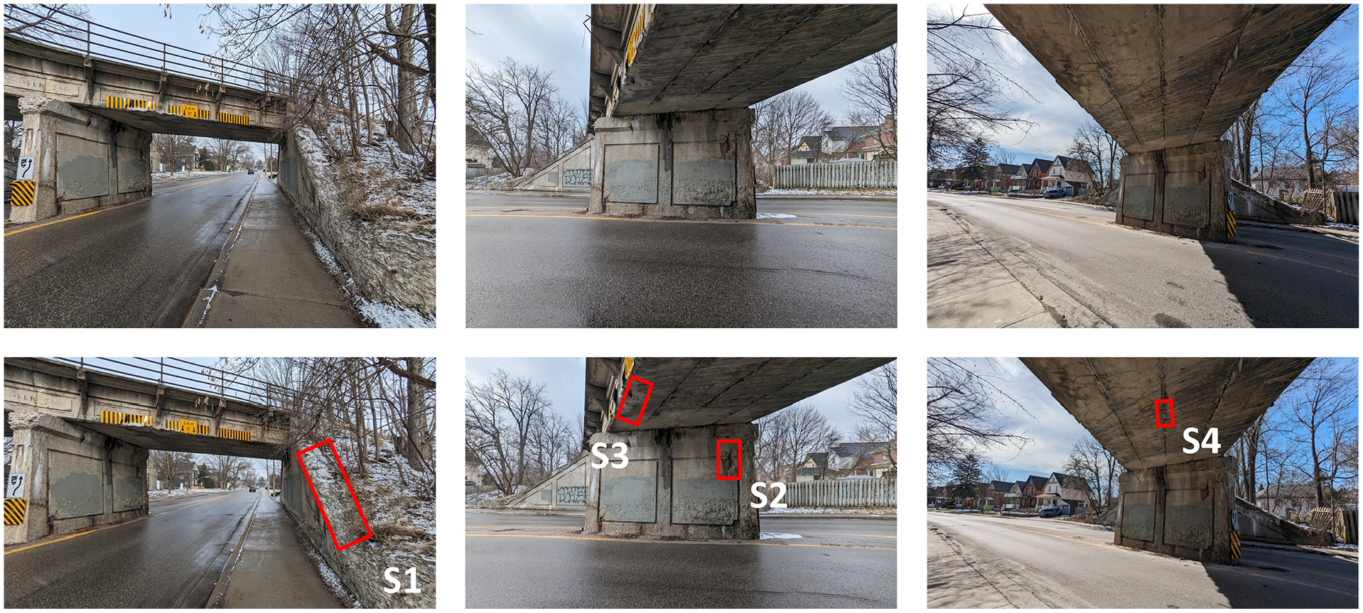
Raw (top) and augmented (bottom) images collected from Google Pixel 6a: S1-S4 are the spalling defects for evaluating quantification performance
Spalling measurements in (mm) from Google Pixel 6a images using ZOE.
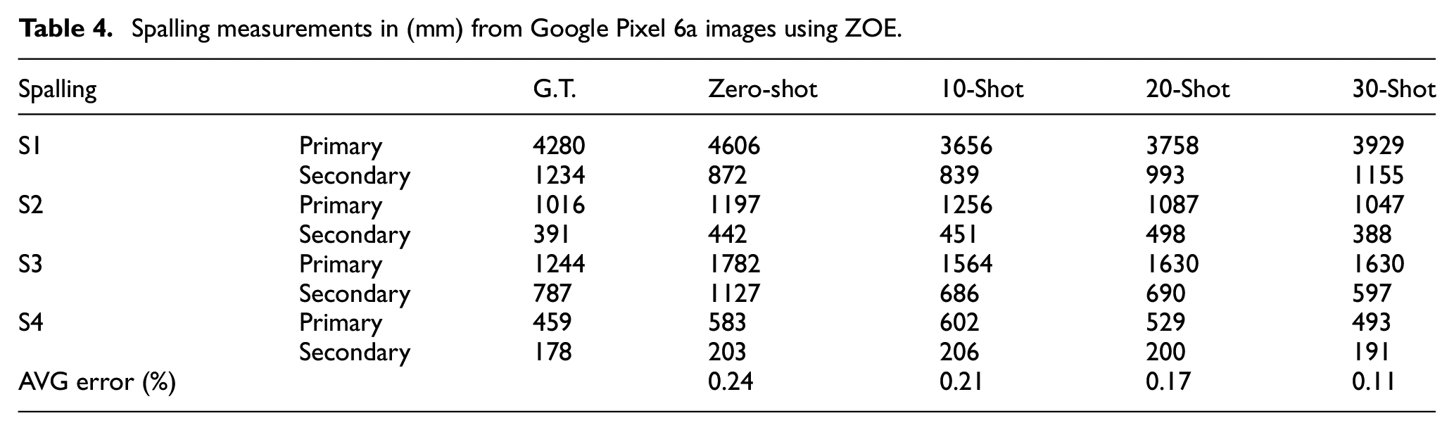
Despite previously transforming the camera intrinsics of the Pixel 6a, there exists many perceivable (i.e., sharpness, contrast, lighting, etc.) and imperceivable (i.e., rolling shutter, postprocessing artifacts) differences between Intel Realsense images. Due to the challenges to synchronize the camera a LiDAR, the training set only contains Intel Realsense RGBD frames, so we expect the depth estimation and thus defect measurement on Pixel 6a images to be worse. On average, we found there is a minor increase in measurement error between the Intel Realsense and Pixel 6a images. However, there are many confounding variables such as the time of day and relative position of the camera that can produce unexpected results. For example, we found that the zero-shot and 10-shot prediction of S4 is improved when using the Pixel 6a, which we believe is likely due to the greater dynamic range of the image and the image containing more of the pier and road, which likely helped the depth estimation. 39 This implies that a higher-quality camera can be beneficial to the future development of the mobile LiDAR system for collecting civil RGB-D data.
In summary, novel developments in monocular depth estimation can be an effective method to measure defects from single images with considerable accuracy. In this work, we focus on the ability of a monocular depth estimation model to generalize, as we believe generalizability is the biggest challenge for real-world application of monocular depth estimation in the civil domain. This is because there is a great diversity of structures in the civil domain and often a high cost to collect spatial data of those structures. In other words, models with high generalizability allow us to make the most of limited data, and we are optimistic that through collaboration with the research community, we can develop a more extensive civil RGB-D dataset. Such that, through this effort, we can facilitate a broad range of monocular depth estimation applications and research within the civil sector.
Conclusion
Defect quantification is an important part of visual structural inspections as it informs defect severity and repair cost estimates. In this work, it is shown that monocular depth estimation can be used to quantifing spalling defects from only a single images. This is enabled by a civil RGB-D dataset, collected using a custom 3D mobile LiDAR scanner. The civil RGB-D dataset is used to evaluate model generalizability performance of two metric monocular depth estimation models: BTS and ZOE. It was experimentally found that ZOE, based on a large vision-transformer model, significantly outperformed BTS, a CNN model, in zero-shot and few-shot configurations. The high generalizability characteristics of ZOE make it most suitable for civil domain applications, where RGB-D data of civil infrastructures is expensive to collect, and the diversity of the infrastructures is large. Lastly, the few-shot ZOE models were used to measure the size of the spalling damages, which were compared to the LiDAR measured ground-truth. While the measurement accuracies are fit for function, there is room for improved with additional training sequences, ZOE-like models with higher generalizability, and better hardware.
Depth estimation has many applications in the civil domain, such as semantic segmentation, path planning, localization. We hope that other researchers will share their scan data to create a comprehensive spatial civil infrastructure dataset to advance the development of vision-based infrastructure inspections.
Supplemental Material
sj-pdf-1-shm-10.1177_14759217251316532 – Supplemental material for Learning monocular depth estimation for defect measurement from civil RGB-D dataset
Supplemental material, sj-pdf-1-shm-10.1177_14759217251316532 for Learning monocular depth estimation for defect measurement from civil RGB-D dataset by Max Midwinter, Zaid Abbas Al-Sabbag, Rishabh Bajaj and Chul Min Yeum in Structural Health Monitoring
Footnotes
Declaration of conflicting interests
The author(s) declared no potential conflicts of interest with respect to the research, authorship, and/or publication of this article.
Funding
The author(s) disclosed receipt of the following financial support for the research, authorship, and/or publication of this article: We acknowledge the support from Rogers Communications, Mitacs through Mitacs Accelerate Program, and the Natural Sciences and Engineering Research Council of Canada [RGPIN-2020-03979].
Supplemental material
Supplemental material for this article is available online.
References
Supplementary Material
Please find the following supplemental material available below.
For Open Access articles published under a Creative Commons License, all supplemental material carries the same license as the article it is associated with.
For non-Open Access articles published, all supplemental material carries a non-exclusive license, and permission requests for re-use of supplemental material or any part of supplemental material shall be sent directly to the copyright owner as specified in the copyright notice associated with the article.