Sage Journals: Discover world-class research

Abstract

Self-supervised learning is a reliable learning mechanism in which a robot uses an original, trusted sensor cue for training to recognize an additional, complementary sensor cue. We study for the first time in self-supervised learning how a robot’s learning behavior should be organized, so that the robot can keep performing its task in the case that the original cue becomes unavailable. We study this persistent form of self-supervised learning in the context of a flying robot that has to avoid obstacles based on distance estimates from the visual cue of stereo vision. Over time it will learn to also estimate distances based on monocular appearance cues. A strategy is introduced that has the robot switch from flight based on stereo to flight based on monocular vision, with stereo vision purely used as “training wheels” to avoid imminent collisions. This strategy is shown to be an effective approach to the “feedback-induced data bias” problem as also experienced in learning from demonstration. Both simulations and real-world experiments with a stereo vision equipped ARDrone2 show the feasibility of this approach, with the robot successfully using monocular vision to avoid obstacles in a 5 × 5 m room. The experiments show the potential of persistent self-supervised learning as a robust learning approach to enhance the capabilities of robots. Moreover, the abundant training data coming from the own sensors allow to gather large data sets necessary for deep learning approaches.

Keywords

Persistent self-supervised learning stereo vision monocular depth estimation robotics

Introduction

It is generally acknowledged that robots operating in the real world benefit greatly from learning mechanisms. Learning allows robots to adapt to environments or circumstances not specifically foreseen at design time. However, the outcome of learning and its influence on the learning robot’s behavior can by definition not be predicted completely. This is a major reason for the delay in introducing successful learning methods such as Reinforcement Learning (RL) in the real world. For instance, with RL it is a major challenge to ensure an exploratory behavior that is safe for both the robot and its environment.¹

Learning from demonstration (LfD) can in this respect be regarded as more reliable. However, in the case of a mobile robot, LfD faces a “feedback-induced data bias” problem.^2,3 If the robot executes its trained policy on real sensory inputs, its actions will be slightly different from the expert’s. As a result, the trajectory of the robot will be different to when the human expert was in control, leading to a test data distribution that is different from the training distribution. This difference worsens the performance of the learned policy, further increasing the discrepancy between the data distributions. The solution proposed in Ross et al.^2,3 is to have the human expert provide novel training data for the sensory inputs experienced by the robot when being in control itself. This leads to an iterative process that requires quite a time investment of the human expert.

There is a relatively new learning mechanism for robots that combines reliability with the advantage of not needing any human supervision. Self-supervised learning (SSL) does not learn a control policy as LfD and RL, but rather focuses on improving the sensory inputs used in control. Specifically, in SSL, the robot uses the outputs of an original, trusted sensor cue to learn recognizing an additional, complementary sensor cue. The reliability comes from the fact that the robot has access to the trusted cue during the entire learning process, ensuring a baseline performance of the system.

Until now, the purpose of SSL has mostly been the exploitation of the complementarity between the sensor cues. To illustrate, perhaps the most well-known example is the use of SSL on Stanley, the car that won the grand DARPA challenge.⁴ Stanley used a laser scanner to detect the road ahead. The range of the laser scanner was rather limited, which placed a considerable restriction on the robot’s driving speed. SSL was used in order to extend the road detection beyond the range of the laser scanner. In particular, the laser scanner-based road classifications were used to train a color model of drivable terrain in the images from a camera. This color model was then applied to image regions not covered by the laser scanner. These image regions higher up in the image allowed to detect the road further away. The use of SSL permitted Stanley to speed up considerably and was an important factor in winning the competition.

A characterizing feature of many of the earlier SSL studies,^4–10 is that the complementary cue is always used in combination with the original sensor cue. More recent studies aim to replace the function of the original cue with that of the complementary cue.^11–14 For instance, in Baleia et al.,¹¹ the sense of touch is used to teach a vision process how to recognize traversable paths through vegetation with the goal of gradually reducing time-intensive haptic interaction. Hence, the learning of recognizing the complementary cue will have to persist in time. However, the consequences of this persistent form of SSL on the robot’s behavior when acting on the complementary cue have not been addressed in the above-mentioned studies.

The main contribution of this article is that we perform an in-depth study of the behavioral aspects of persistent SSL. We do so in the context of a scenario in which the robot should keep performing its task even when the supervisory cue becomes completely unavailable. Importantly, when the robot relies only on the complementary cue, it will encounter the feedback-induced data bias problem known from LfD. We suggest a novel behavior strategy during learning to handle this problem in persistent SSL. Specifically, we study a flying robot with a stereo vision system that has to avoid obstacles in a global positioning system (GPS)-denied environment. The robot uses SSL to learn a mapping from monocular appearance cues to stereo-based distance estimates. We have chosen this context because it is relevant for any stereo-based robot that needs to be robust to a permanent failure of one of its cameras. In computer vision, monocular distance estimation is also studied. There, the main challenges are the gathering of sufficient data (e.g., for deep neural networks) and the generalization of the learned distance estimation to an unforeseen operation environment. Both of these challenges are addressed to some extent by SSL, as learning data are abundant and the robot learns in the environment in which it operates. We regard SSL as an important supplement to machine learning for robots. Therefore, we end the study with a discussion on the position of (persistent) SSL in the broader context of robot and machine learning, comparing it among others with RL, LfD, and supervised learning.

The remainder of the article is set up as follows. First, we discuss related work. Then, we more formally introduce persistent SSL and explain our implementation for the stereo-to-mono learning. We analyze the similarity of the specific SSL case studied in this article with LfD approaches. Subsequently, we perform offline vision experiments in order to assess the performance of various parameter settings. Thereafter, we compare various learning strategies in simulation. The best learning strategy is implemented for experiments with a Parrot ARDrone2, and the results of these robotic experiments are analyzed. Finally, the broader implications of the findings on persistent SSL are discussed, and conclusions are drawn.

Related work

We study persistent SSL in the context of a stereo-vision equipped robot that has to learn to navigate with a single camera. In this section, we discuss the state-of-the-art in the most relevant areas to the study: monocular navigation and SSL.

Monocular navigation

The large majority of monocular navigation approaches focuses on motion cues. The optical flow of world points allows for the detection of obstacles¹⁵ or even the extraction of structure from motion, as in monocular simultaneous localization and mapping (SLAM).¹⁶ The main issue of using monocular motion cues for navigation is that optical flow only conveys information on the ratio between distance and the camera’s velocity. Additional information is necessary for retrieving distance. This information is typically provided by additional sensors,¹⁶ but can also be retrieved by performing specific optical flow maneuvers.^17,18

In contrast, it is well known that the appearance of objects in a single, still image does contain distance information. Successfully estimating distances in a single image allows robots to evaluate distances without having to move. In addition, many appearance extraction and evaluation methods are computationally efficient. Both these factors can aid the robot in the making of quick navigation decisions. Below, we give an overview of work in the area of monocular appearance-based distance estimation and navigation.

Appearance-based navigation without distance estimation

There are some appearance-based navigation methods that do not involve an explicit distance estimate. For instance, in de Croon et al.,¹⁹ an appearance variation cue is used to detect the proximity to obstacles, which is shown to be successful at complementing optical flow-based time-to-contact estimates. A threshold is set that makes the flying robot turn if the variation drops too much, which will lead to turns at different distances.

An alternative approach is to directly learn the mapping from visual inputs to control actions. In order to fly a quad rotor through a forest, Ross et al.³ use a variant of LfD²⁰ to acquire training data on avoiding trees in a forest. First a human pilot controls the drone, creating a training data set of sensory inputs and desired actions. Subsequently, a control policy is trained to mimic the pilot’s commands as good as possible. This control policy is then implemented on the drone.

A major problem of this approach is the feedback-induced data bias: A robot has a feedback loop of actions and sensory inputs, so its control policy determines the distribution of world states that it encounters (with corresponding sensory inputs and optimal actions). Small deviations between the trained controller and the human may bring the robot in unknown states for which it has received no training. Its control policy may generalize badly to such situations. The solution proposed in Ross et al.³ is a transitional model called DAgger,² in which actions from the expert are mixed with actions from the trained controller. In the real-world experiments in Ross et al.,³ several iterations have been performed in which the robot flies with the trained controller, and the captured videos are labeled offline by a human. This approach requires skilled pilots and significant human effort.

Many current studies focus on using deep RL²¹ to learn a mapping from images to actions. One of the most successful current attempts is the work in Sadeghi and Levine,²² which learns a deep neural network completely in simulation and then ports the network to a real robot in a yet unseen environment. The trained network performs quite admirably in the real environment. Key to the success of learning is to ensure a large variety of textures, lighting, and obstacle arrangements in simulation. Of course, if the real environment is still very different from the training environments, performance can degrade considerably.

Offline monocular distance learning

Humans are able to see distances in a single still image, and there is a growing body of work in computer vision utilizing machine learning to do the same. Interest in single image depth estimation was sparked by work from Hoiem et al.²³ and Saxena et al.^24,25 Hoiem’s automatic photo pop-up tries to group parts of the image into segments that can be popped up at different depths. Saxena’s Make-3D uses a Markov random field (MRF) approach to classify a depth per image patch on different scales. These studies focus on creating a dense depth map with a machine learning computer vision approach. Both methods use supervised learning on a large training data set. Some work was done on adopting variants of Saxena’s MRF work for driving rovers and even for MAVs. Lenz et al.²⁶ proposed a solution based on a MRF to detect obstacles on board an MAV, but it does not infer how far the objects are. Instead, it is trained offline to recognize three different obstacle class types. Any different objects could hence lead to navigation problems.

Recently, again focusing on creating a dense depth map from a single image, Eigen et al.²⁷ propose a multi-scale deep neural network approach trained on the KITTI data set, making it more resilient for practical robot data. Training deep neural networks require a large data set, which is often obtained by deforming training data or by artificially generating training data. Michels et al.²⁸ use artificial data to learn recognizing obstacles on a rover, but in order to generalize well it requires the use of a very realistic simulator. In addition, the same work reports significant improvement if the artificial data are augmented with labeled real-world data.

Other groups acquire training data for supervised learning by having another separate robot or system acquire data. This data are then processed and learned offline, after which the learned algorithm is deployed on the target robot. Dey et al.²⁹ use an RC car with a stereo vision setup to acquire data from an environment, apply machine learning on this data offline, and navigate a similar but unseen environment with an MAV based on the trained algorithm. Creating and operating a secondary system designed to acquire training data, however, is no free lunch. Moreover, it introduces inconvenient biases in the training data, because an RC car will not behave in a similar way both in terms of dynamics, camera viewpoint, and the path chosen through the environment.

None of the above methods have the robot gather the data and learn while in operation.

Self-supervised learning

The idea of SSL has been around since the late 1990s,³⁰ but the successful application of it to terrain classification on the autonomously driving car Stanley³¹ demonstrated its first major practical use. A similar approach was taken by Hadsell et al.,⁹ but now using a stereo vision system instead of a LIDAR system, and complex convolutional filters instead of simple and fixed color-based features. These approaches largely forgo the need for manually labeled data as they are designed to work in unseen environments.

In most studies on SSL for terrain classification, the ground truth is always used during operation. In contrast, two very recent studies have as goal that the robot takes some decisions based on the complementary sensor cue alone. Since the complementary cue then has to persist in the absence of the original cue, this form of SSL can be termed “persistent SSL.” Baleia et al.¹¹ study a rover with a haptic antenna sensor. In their application of terrain mapping, they try to map monocular cues to obstacles based on earlier events of encountering similar situations that resulted in either a hard obstacle, a traversable obstacle, or a clear path. The monocular information is used in a path-planning task, requiring a cost function for either exploring unknown potential obstacles or driving through a terrain on the current available information. Since checking whether a potential obstacle is traversable is costly (the rover needs to travel there in order for the antenna to provide ground truth on that), the robot learns to classify the terrain ahead with vision. On each sample an analysis is performed to determine whether the vision-based classifier is sufficiently confident: it either decides the terrain is traversable, not traversable, or unsure. In the unsure case, the sample is sensed using the antenna. Gradually this will become necessary less often, thus learning to navigate using its Kinect sensor alone. In Ho et al.,¹² a flying robot first uses optical flow to select a landing site that is flat and free of obstacles. In order for this to work, the robot has to move sufficiently with respect to the objects on the landing site. While flying, the robot uses SSL to learn a regression function that maps an (appearance-based) texton distribution to the values coming from the optical flow process. The learned function extends the capabilities of the robot, as after learning it is also able to select landing sites without moving (from hover). The article shows that if the robot is uncertain on its appearance-based estimates, it can switch back to the original optical flow-based cue.

The main contribution of this article is that we focus on the behavioral aspects of persistent SSL. We study how to best set up the behavior during the learning process, so that the robot will be able to keep performing its task when the original sensor cue becomes completely unavailable. Furthermore, we use stereo vision as the trusted, original cue, something which has not been done before in SSL. Concerning a comparison with the largest body of work on SSL that deals with terrain traversability classification, learning depth estimates directly is likely more complex. To illustrate, the robot would not only have to recognize sand, but it also has to make the difference between sand at 1-m distance and at 3-m distance. As mentioned above though, successful algorithms exist even to estimate complete dense depth maps from single images. In this article, since the emphasis is on behavior, we will deal with simplified environments and the estimation is restricted to the average depth in the field of view of the camera.

Methodology overview

In this section, we describe the persistent SSL learning mechanism and describe our implementation of this mechanism for our specific proof of concept case, monocular depth estimation in flying robots. Note that since our interest is in the behavioral aspects of persistent SSL, it is most important that the robot flies and learns in real time. Moreover, for the applicability to small flying robots, it is important that the processing for such SSL can be performed onboard, even considering the significant restrictions in onboard processing. The focus here is not yet on dealing with complex environments or on the accomplishment of missions like exploration or navigation. In this study, we investigate a very simple environment and obstacle avoidance behavior. We end this section with a description of the three learning behaviors that we compare with each other.

Persistent SSL principle

The persistent SSL principle is schematically depicted in Figure 1. In persistent SSL, an original, pre-wired sensory cue provides supervised outputs to a learning process that takes a different, complementary sensory cue as input. The goal is to be able to replace the pre-wired cue if necessary. When considering the system as a whole, learning with persistent SSL can be considered as unsupervised; it requires no manual labeling or pre-training before deployment in the field. Internally it uses a supervised learning method that in fact needs ground truth labels to learn. This ground truth is, however, assumed to be provided online and autonomously without human or outside interference.

Figure 1.

The persistent self-supervised learning principle.

In the schematic, the input variable x represents the sensory inputs available on board. The variables x_g and x_f are possibly overlapping subsets of these sensory inputs. In particular, function $g (x_{g})$ extracts a trusted ground truth sensory cue from the sensory inputs x_g. In classical systems, $g (x_{g})$ provides the required functionality on its own:

g : x_{g} \to y, x_{g} \subseteq x

(1)

The function $f (x_{f})$ is learned with a supervised learning algorithm in order to approximate $g (x_{g})$ based on x_f:

f : x_{f} \to \hat{y}, f \in F, x_{f} \subseteq x

(2)

\hat{f} = \underset{f \in F}{argmin} E [l (f (x_{f}), g (x_{g}))]

(3)

where

l (f (x_{f}), g (x_{g}))

is a suitable loss function that is to be minimized. The system can either choose or be forced to switch θ, so that λ is either set to

g (x_{g})

\hat{f} (x_{f})

for use in control. Future work may also include fusing the two, but in this article, we focus on using the complementary cue in a stand-alone fashion. It must be noted that while both

x_{g} \subseteq x

and

x_{f} \subseteq x

, in general it may be that x_f does not contain all necessary information to predict y. In addition, even if x_g = x_f, it is possible that F does not contain a function f that perfectly models g. The information in x_f and the function space F may not allow for a perfect estimate of

g (x_{g})

. On the other hand, there may be an

f (x_{f})

that handles certain situations better than

g (x_{g})

(think of landing site selection from hover, as in Ho et al.¹²). In any case, fundamental differences between

g (x_{g})

and

\hat{f} (x_{f})

are to be expected, which may significantly influence the behavior when switching θ. Handling these differences is of central interest in this article.

Stereo-to-mono proof of concept

Figure 2 presents a block diagram of the proposed proof of concept system in order to visualize how the persistent SSL method is employed in our application: estimating monocular depth with a flying robot. Input is provided by a stereo vision camera, with either the left or right camera image routed to the monocular estimator. We use a Visual Bag of Words (VBoW) method for this estimator. The ground truth for persistent SSL in this context is provided by the output of a stereo vision algorithm. In this case, the average value of the disparity map is used, both for training the monocular estimator and as an input to the switch θ. Based on the switch, the system either delivers the monocular or the stereo vision average disparity to the behavior controller.

Figure 2.

System overview. See the text for details.

Stereo vision processing

The stereo camera delivers a synchronized gray-scale stereo-pair image per time sample. A stereo vision algorithm first computes a disparity map, but often this is a far from perfect process. Especially in the context of an MAV’s size, weight and computational constraints, errors caused by imperfect stereo calibration, resolution limits, etc. can cause large pixel errors in the results. Moreover, learning to estimate a dense disparity map, even when this is based on a high quality and consistent data set, is already very challenging. Since we use the stereo result as ground truth for learning, we minimize the error by averaging the disparity map to a single scalar. A single scalar is much easier to learn than a full depth map and has been demonstrated to provide elementary obstacle avoidance capability.^28,32,33

The disparity λ relates to the depth d of the input image:

d \propto \frac{1}{λ}

(4)

Using averaged disparity instead of averaged depth fits the obstacle avoidance application better, because small but close by objects are emphasized due to the nonlinear relation of equation (4). However, linear learning methods may have difficulty mapping this relation. In our final design, we thus choose to learn the disparity with a nonparametric approach, which is resilient to nonlinearities.

Monocular disparity estimation

The monocular disparity estimator forms a function from the image’s pixel values to the average disparity in the image. Since the main goal of the article is to study SSL on board a drone in real time, efficiency of both the learning and execution of this function is very important. Hence, we converged to a computationally extremely efficient VBoW approach for the robotic experiments. We have also explored a deep neural network approach, but the hardware and time available for learning did not allow for having the deep neural learning on board the drone at this stage.

The VBoW method uses small image patches of w × h pixels, as successfully introduced in Varma and Zisserman³⁴ for a complex texture classification problem. First, a dictionary is created by clustering the image patches with Kohonen clustering (as in De Croon et al.³³). The n cluster centroids are called “textons.” In this work, two types of textons are used: normal intensity textons and gradient textons obtained similarly but based upon the gradient of the images. Gradient textures have been shown in Wu et al.³⁵ to be an important depth cue. An example dictionary of each is depicted in Figure 3. Gradient textons are shown with a color range (from blue = low, to red = high). The intensity textons in Figure 3 are based on grayscale intensity pixel values.

Figure 3.

The texton library used in the experiments. The right set of textons is based on pixel intensities, the left set contains (artificially colored) gradient textons (i.e., textons based on gradient images).

When an image is received, m patches are extracted from the W × H pixel image. Each patch is compared to the dictionary by means of a distance function, in order to form a texton occurrence histogram for the image; the texton bin with the smallest Euclidean distance to a given patch is increased by 1. The histogram is normalized to sum to 1. Then, each normalized histogram is supplemented with its Shannon entropy, resulting in a feature vector of size n + 1. The idea behind adding the entropy is that the variation of textures in an image decreases when the camera gets closer to obstacles.³³ To illustrate the change in texton histograms when approaching an obstacle, a time series of texton histograms can be seen in Figure 4. Note how the entropy of the distribution indeed decreases over time, and that especially the fourth bin is much higher when close to the poster on the wall. A machine learning algorithm will have to learn to notice such relationships itself for the robot’s environment, by learning a mapping from the feature vector to a disparity scalar. We have investigated different function representations and learning methods to this end.

Figure 4.

Approaching a poster on the wall. Left: monocular input. Middle: overlaid textons annotated with the color used in the histogram. Right: texton distribution histogram with the corresponding texton shown beneath it.

Control behavior

The proposed system uses a straightforward behavior heuristic to explore, navigate, and persistently learn a room. The heuristic is depicted as a finite state machine (FSM) in Figure 5. The FSM detects obstacles by means of a threshold t applied to the average disparity λ. In state 0, the robot flies in the direction of the camera’s principal axis. When an obstacle is detected ( $λ > t$ ), the robot stops and goes to state 1 in which it randomly chooses a new direction for the principal axis. It immediately passes to state 2 in which the robot rotates toward the new direction, reducing the error e between the principal axis’ current and desired direction. If in the new direction obstacles are far enough away ( $λ \leq t$ ), the robot starts flying forward again (state 0). Else, the robot continues to turn in the same direction as before (clockwise or counter clockwise) until $λ \leq t$ . When this is the case, it starts flying straight again (state 0). Choosing this rather straightforward behavior heuristic enables autonomous exploration based on only one scalar obtained from a distance sensor.

Figure 5.

The behavior heuristic FSM. λ is average disparity, e is the attitude error (meaning the difference between the newly picked direction and the current attitude), t_n the respective thresholds.

Performance

The average disparity λ, coming either from stereo vision or from the monocular distance estimation function $f (x_{f})$ , is thresholded for determining whether to turn. This leads to a binary classification problem, where all samples for which $λ > t$ are considered as “positive” (c = 1) and all samples for which $λ \leq t$ are considered as “negative” (c = 0). Hence, the quality of $\hat{f} (x_{f})$ can be characterized by a receiver operating characteristic (ROC) curve. The ground truth for the ROC curve is determined by the stereo vision. This means that a true positive ratio (TPR) of 1 and false positive ratio (FPR) of 0 lead to the same obstacle detection performance as with the stereo vision system. Generally, of course, this performance will not be reached, and the robot has to determine what threshold to set for a sufficiently high TPR and low FPR.

This leads to the question how to determine what a “sufficient” TPR/FPR is. We evaluate this matter in the context of the robot’s obstacle avoidance task. In particular, we first look at the probability of a collision with a given TPR and then at the probability of a spurious turn with a given FPR.

In order to model the probability of a collision, consider a constant velocity approach with input samples (images) $〈 x_{1}, x_{2}, \dots, x_{n} 〉$ of n samples long, ending at an obstacle. A minimum of u samples before actual impact, an obstacle must be detected by at least one TP or a FP in order to prevent a collision. Since the range of samples $〈 x_{(n - u + 1)}, x_{(n - u + 2)}, \dots, x_{n} 〉$ does not matter for the outcome, we redefine the approach range to be $〈 x_{1}, x_{2}, \dots, x_{(n - u)} 〉$ . Consider that for each sample x_i holds:

1 = p (T P | x_{i}) + p (F P | x_{i}) + p (T N | x_{i}) + p (F N | x_{i}),

(5)

since

p (F N | x_{i}) = p (T P | x_{i}) = 0

if x_i is a negative and

p (T N | x_{i}) = p (F P | x_{i}) = 0

if x_i is a positive. Let us first assume independent, identically distributed (i.i.d.) data. Then, the probability of a collision p_c can be written as:

\begin{array}{l} p_{c} = \prod_{i = 1}^{n - u} (p (F N | x_{i}) + p (T N | x_{i})) \\ = \prod_{i = 1}^{q} p (T N | x_{i}) \prod_{i = q + 1}^{n - u} p (F N | x_{i}), \end{array}

(6)

where q is a time step separating two phases in the approach. In the first phase all x_i are negative, so that any false positive will lead to a turn, preventing the collision. Only if all negative samples are correctly classified as negatives (true negatives), will the robot enter the second phase in which all x_i are positive. Then only a complete sequence of false negatives will lead to a collision, since any true positive will lead to a timely turn.

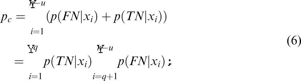
We can use equation (6) to choose an acceptable $T P R = 1 - F N R$ . Assuming a constant velocity and frame rate, it gives us the probability of a collision. For instance, let us assume that the robot flies forward at 0.50 m/s with a frame rate of 30 Hz. To avoid collisions, it has a minimal required detection distance of 1.0 m, while “positives” are defined to be closer than 1.5 m. This leads to 0.5 m of flight during which the robot can detect an oncoming collision, corresponding to s = 30 samples that all have to be classified as (false) negatives for a collision to occur. In the case of i.i.d. data, if we think a probability $p_{c} \leq 10^{- 6}$ is acceptable, then the desired $T P R \geq 1 - 2 ({log}_{2} (10^{- 6}) / 30) \sim 0.369$ .

The analysis of the effect of false positives is straightforward, as it can be expressed in the number of spurious turns per second or, equivalently if assuming a constant velocity, per meter traveled. With the same scenario as above, an FPR = 0.05 will on average lead to three spurious turns per traveled meter, which is unacceptably high. An FPR = 0.0017 will approximately lead to 1 spurious turn per 10 m.

The above analysis seems to indicate that quite many false negatives are acceptable, while there can only be very few false positives. However, there are two complicating factors. The first factor is that equation (6) only holds when X can be assumed i.i.d., which is unlikely due to the nature of the consecutive samples of an approach toward an obstacle. Some reasoning about the nature of the dependence is, however, possible. Assuming a strong correlation between consecutive samples results in a higher probability of x_i being classified the same as $x_{(i + 1)}$ . In other words, if a sample in the range $〈 x_{1} .. x_{m} 〉$ is an FN, the chance increases that more samples are FNs. Hence, the expected dependencies significantly impact performance of the system making equation (6a) best case scenario for FNs and a worst case scenario for FPs.

The system can be more realistically modeled as a Markov process as depicted in Figure 6. From this it can be seen that the system can be split in a reducible Markov process with an absorbing avoid state, and a chain of states that leads to the absorbing collision state. The values of the transition matrix Ω can be determined from the data gathered during operation. This would allow the robot to better predict the consequences of a chosen TPR and FPR.

Figure 6.

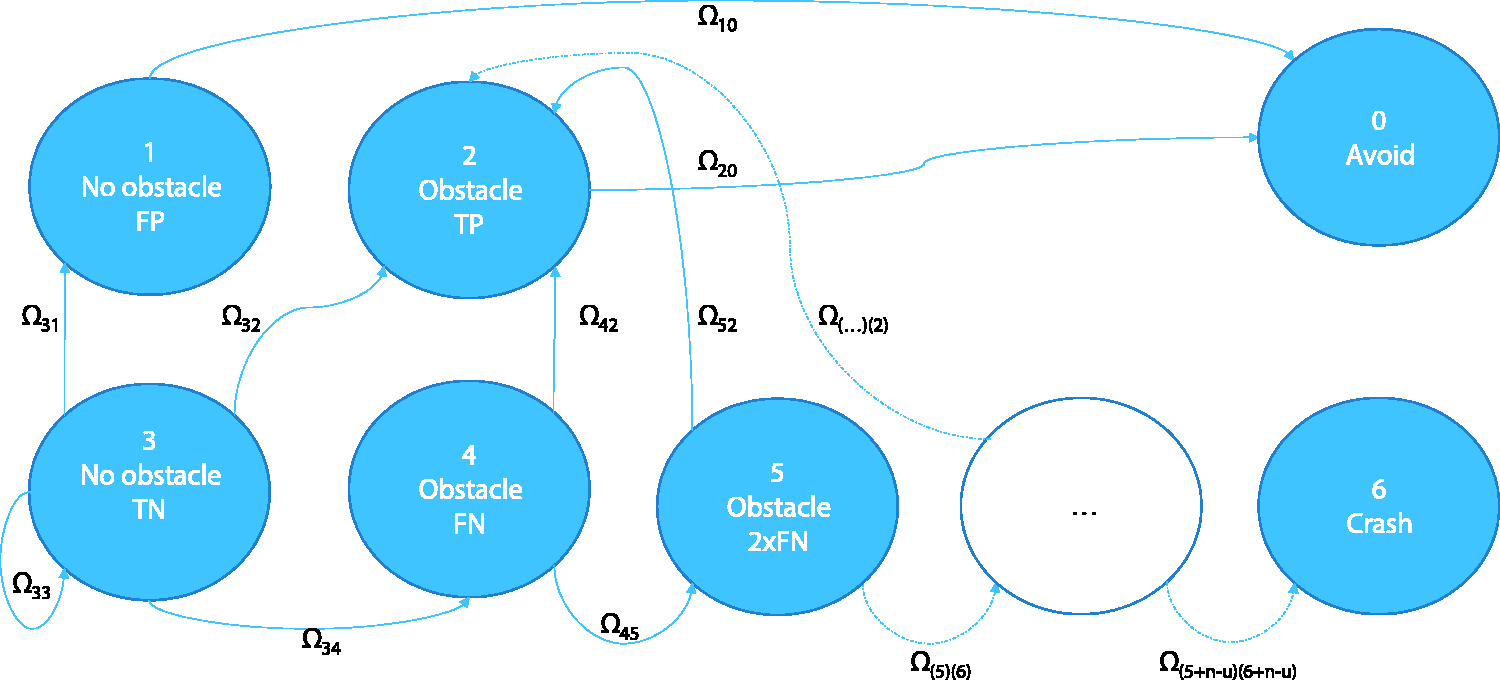
A Markov model of the probability of a collision. Due to the nature of the consecutive samples, state transition probabilities $Ω_{(5 + n) (6 + n + u)}$ are not equal to $Ω_{(3) (4)}$ but are likely to be relatively high. (Once one frame was wrongly classified as no obstacle, it is likely the upcoming frames will also be wrongly classified as they are similar.)

As an illustration of the effects of sample dependence, let us suppose a model in which each classification has a probability of being identical to the previous classification, $p (I (c_{i - 1}, c_{i}))$ . If not identical, the sample is classified independently. This dependency model allows us to calculate the transition $Ω_{4, 5}$ in Figure 6. Given a previous negative classification, the transition probability to another negative classification is: $Ω_{4, 5} = p (I (c_{i - 1}, c_{i})) + (1 - p (I (c_{i - 1}, c_{i}))) (1 - T P R)$ . If $p (I (c_{i - 1}, c_{i})) = 0.8$ and TPR = 0.95, $Ω_{4, 5} = 0.81$ . The probability of a collision in such a model is $p_{c} = Ω_{4, 5}^{(s - 1)} = 1.8 10^{- 3}$ , no longer an inconceivably small number.

This leads us to the second complicating factor, which is specific to our SSL setup. Since the robot operates on the basis of the ground truth, it should theoretically hardly ever encounter positive samples. Namely, the robot should turn when it detects a positive sample. This implies that the uncertainty on the estimated TPR is rather high, while the FPR can be estimated better. A potential solution to this problem is to purposefully have the mono-estimation robot turn earlier than the stereo vision-based one.

Similarity with LfD

The core of SSL is a supervised algorithm that learns the function $\hat{f} (x_{f})$ on the basis of supervised outputs $g (x_{g})$ . Normally, supervised learning assumes that the training data are drawn from the same data probability distribution $D$ as the test data. However, in persistent SSL, this assumption generally does not hold. The problem is that by using control based on $\hat{f}$ , the robot follows a control policy $π_{\hat{f}} \neq π_{g}$ and hence will induce a different state distribution, $D_{π_{\hat{f}}} \neq D_{π_{g}}$ . On these different states, no supervised outputs have been observed yet, which typically implies an increasing difference between $\hat{f}$ and g.

A similar problem of inducing a different state distribution is well known in the area of LfD.^2,3 Actually, we will show that under some mild assumptions, the persistent SSL problem studied in this paper is equivalent to an LfD problem. Hence, we can draw on solutions in LfD such as DAgger.²

The goal of LfD is to find a policy $\hat{π}$ that minimizes a loss function l under its induced distribution of states, from Ross et al.²:

\hat{π} = \underset{π \in Π}{argmin} E_{s \sim D_{π}} [l (s, π)]

(7)

where an optimal, teacher policy

π^{*}

is available to provide training data for specific states s.

At first sight, SSL is quite different, as it focuses only on the state information that serves as input to the policy. Instead of optimizing a policy, the supervised learning in persistent SSL can be defined as finding the function $f'$ that best matches the trusted function $g'$ under the distribution of states induced by the use of the thresholded version f for control:

\underset{f \in F}{argmin} E_{x \sim D_{π_{f}}} [l (f (x), g (x))]

(8)

meaning that we perform regression of f on states that are induced by the control policy π_f, which uses the thresholded version of f.

To see the similarity to equation (7), first realize that the stereo-based policy is in this case the teacher policy: $π_{g} = π^{*}$ . For this analysis, we simplify the strategy to flying straight when far enough away from an obstacle, and turning otherwise:

\begin{array}{l} π_{g} (s) : p (straight | s = 0) = 1 \\ p (turn | s = 1) = 1 \end{array}

(9)

where s is the state, with s = 1 when

g (x) > t_{g}

and s = 0 otherwise. Note that π_g is a deterministic policy, which is assumed to be optimal.

When we learn a function $\hat{f}$ , it generally will not give exactly the same outputs as g. Using $\hat{s} : = \hat{f} > t_{\hat{f}}$ will result in the following stochastic policy:

\begin{array}{l} π_{\hat{f}} (s) : p (straight | s = 0) = T N R \\ p (turn | s = 0) = F P R \\ p (turn | s = 1) = T P R \\ p (straight | s = 1) = F N R \end{array}

(10)

a stochastic policy which by definition is optimal,

π_{\hat{f}} = π_{g}

, if

F P R = F N R = 0

. In addition, then

D_{π_{\hat{f}}} = D_{π_{g}}

. Thus, if we make the assumption that minimizing

l (f (x), g (x))

also minimizes FPR and FNR, capturing any preference for one or the other in the cost function for the behavior

l (s, π)

, then minimizing f in equation (8) is equivalent to minimizing the loss in equation (7).

Learning schemes

The interest of the above-mentioned similarity lies in the use of proven techniques from the field of LfD for training the persistent SSL system. In this article, we study a well-known method from this field, named DAgger,² and compare it with two additional methods. All three learning schemes start with an initial learning period in which the drone is controlled purely by means of stereo vision. The three methods are different though as follows.

In the first learning scheme, the drone will continue to fly based on stereo vision for the remainder of the learning time. After learning, the drone immediately switches to monocular vision. For this reason, the first scheme is referred to as “cold turkey.”

In the second learning scheme, the drone will perform a stochastic policy, selecting the stereo vision-based actions with a probability β_i and monocular-based actions with a probability $(1 - β_{i})$ , as was proposed in the original DAgger article.² In the experiments, $β_{i} = 0.25$ .

In the third learning scheme, the drone will perform monocular-based actions, with stereo vision only used to override these actions when the drone gets too close to an obstacle. Therefore, we refer to this scheme as “training wheels.”

Offline vision experiments

In this section, we perform offline vision experiments. The goal of these experiments is to determine how good the proposed VBoW method is at estimating monocular depth, and to determine the best parameter settings.

To measure the performance, we use two main metrics: the mean square error (MSE) and the area under the curve (AUC) of an ROC curve. MSE is an easy metric that can be directly used as a loss function, but in practice many situations exist in which a low MSE can be achieved while inadequate performance is reached for the basis of reliable MAV behavioral control. The AUC captures the trade-off between TPR and FPR and hence is a good indication of how good the performance is in terms of obstacle detection.

We use two data sets in the experiments. The first data set is a video made on a drone during an autonomous flight using an onboard 128 × 96 pixels stereo camera. The second data set is a video made by manually walking with a higher quality 640 × 480 pixel stereo camera through an office cubicle in a similar fashion as the robot should move in the later online experiments. The data sets #1 and #2 used in this section are made available for download publicly.³⁶ An example image from each data set is shown in Figure 7.

Figure 7.

Example from data set #1 (left, 128 × 96 pixels) and data set #2 (right, 640 × 480).

Our implementation of the VBoW method has six main parameters, ranging from the number of intensity and gradient textons to the number of samples used to smooth the estimated disparity over time. An exhaustive search of parameters being out of reach, we have performed various investigations of parameter changes along a single dimension. Table 1 presents a list of the final tuned parameter values. Note that these parameter values have not only been optimized for performance. Whenever performance differences were marginal, we have chosen the parameter values that saved on computational effort. This choice was guided by our goal to perform the learning on board of a computationally limited drone. Below we will show a few of the results when varying a single parameter, deviating from the settings in Table 1 in the corresponding dimension.

Table 1.

Parameter settings.

Parameter	Value
Number of intensity textons	10
Number of gradient textons	10
Patch size	5 × 5
Subsampling samples	500
kNN	K = 5
Smooth size	4

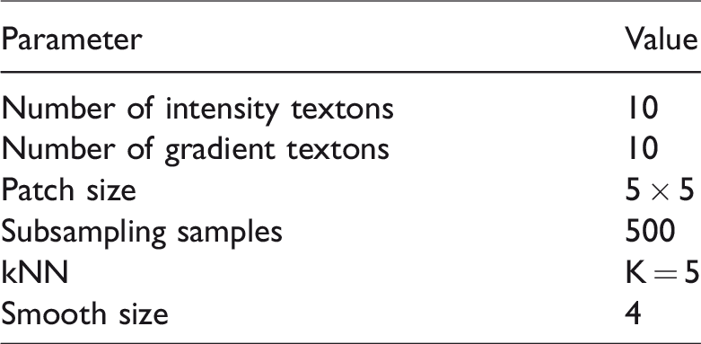
Figure 8 shows the results for different numbers of textons, $\in {4, 8, 12, 16, 20}$ , always consisting half out of pixel intensity and half of gradient textons. From the results, we can see that the performance saturates around 20 textons. Hence we selected this combination of 10 intensity and 10 gradient textons for the experiments.

Figure 8.

MSE and AUC number of textons. Dashed/solid lines refer to results on train/test set.

The VBoW method involves choosing a regression algorithm. In order to determine the best learning algorithm, we have tested four regression algorithms, limiting the choice mainly based on feasibility for implementing the regression algorithm on board a constrained embedded system. We have tested two non-parametric (kNN and Gaussian process regression) and two parametric (linear and shallow neural network regression) algorithms. Figure 9 presents the learning curves for a comparison of these regressors. Clearly, in most cases the kNN regression comes out best. A naive implementation of kNN suffers from having a larger training set in terms of CPU usage during test time, but after implementation on the drone, this did not become a bottleneck.

Figure 9.

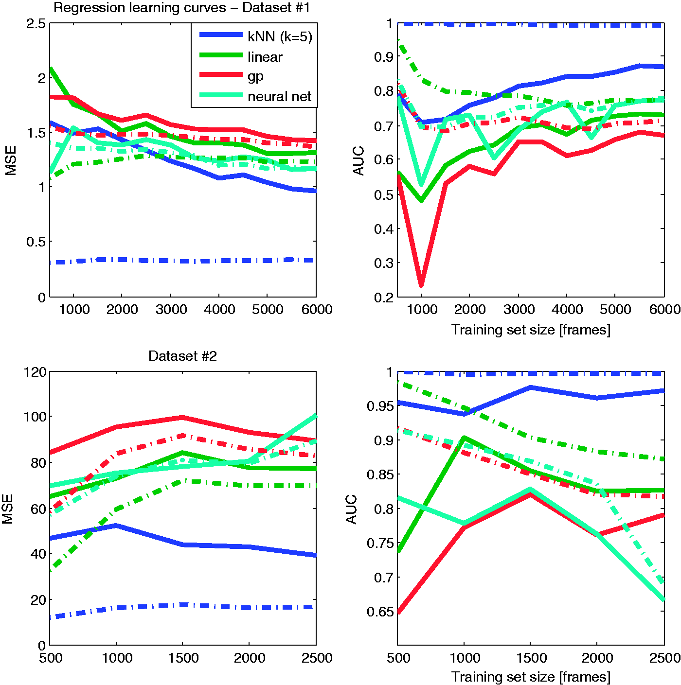
VBoW regression algorithms learning curves. Dashed/solid lines refer to results on train/test set.

The final offline results on the two data sets are quite satisfactory. They can be viewed online (note 1). After a training set of roughly 6000 samples, the kNN approximates the stereo vision-based disparities in the test set rather well. Given a desired TPR of 0.82, the learner has an FPR of 0.26. Considering the high inter-dependability of concurrent frames, this should be sufficient for usage of the estimated disparities in control.

Simulation experiments

We argued that a persistent form of SSL is similar to LfD. The relevance of this similarity lies in the behavioral schemes used for learning. In this section, we compare the three learning schemes, as introduced in the section Learning Schemes, in simulation.

Setup

We simulate a “flying” drone with stereo vision camera in SmartUAV,³⁷ an in-house developed simulator that allows for 3D rendering and simulation of the sensors and algorithms used on board the real drone. Figure 10 shows the simulated “office room.” The room has a size of 10 × 10 m, and the drone has an average forward speed of 0.5 m/s. All the vision and learning algorithms are exactly the same as the ones that run on board of the drone in the real experiments.

Figure 10.

SmartUAV simulation environment.

We compare the three learning schemes, cold turkey, DAgger, and training wheels, in simulation. As mentioned, these schemes all have the same initial training period with stereo vision being in control, but they differ in the remaining learning period. After all learning, the drone will use its monocular disparity estimates for control. The stereo vision remains active only for overriding the control if the drone gets too close to a wall. During this testing period, we register the number of turns and the number of overrides. The number of overrides is a measure of the number of potential collisions. The performed number of turns during testing is compared to the number of turns performed when solely using stereo vision, to evaluate the number of spurious turns. The initial learning period is 1 min, the remaining learning period is 4 min, and the test time is 5 min. These times have been selected to allow a full experiment on a single battery of the real drone.

Results

Table 2 contains the results of 30 experiments with the three learning schemes and a purely stereo-vision-controlled drone. The first observation is that “cold turkey” gives the worst results. This result was to be expected on the basis of the similarity between persistent SSL and LfD: the learned monocular distance estimates do not generalize well to the test distribution when the monocular vision is in control. The originally proposed DAgger scheme performs better, while the third learning scheme termed “training wheels” seems most effective. The third scheme has the lowest number of overrides of all learning schemes, with a similar total number of turns as a pure stereo vision run. The intuition behind this method being best is that it allows the drone to best learn from samples when the drone is beyond the normal stereo vision turning threshold. The original DAgger scheme has a larger probability to turn earlier, exploring these samples to a lesser extent. Double-sided statistical bootstrap tests³⁸ indicate that all differences between the learning methods are significant with p < 0.05.

Table 2.

Test results for the three learning schemes.

Method	Overrides	Turns
Pure stereo	N/A	45.6 ( $σ = 3.0$ )
1. Cold turkey	25.1 ( $σ = 8.2$ )	42.8 ( $σ = 3.7$ )
2. DAgger	10.7 ( $σ = 5.3$ )	41.4 ( $σ = 3.2$ )
3. Training wheels	$4.3$ ( $σ = 2.6$ )	40.4 ( $σ = 2.6$ )

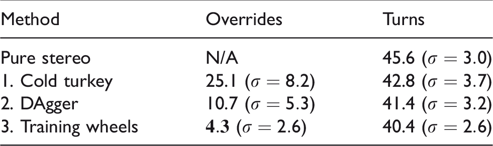
The average and standard deviation are given for the number of overrides and turns during the testing period. A lower number of overrides is better. In the table, the best results are shown in boldface.

The differences between the learning schemes are well illustrated by the positions the drone visits in the room during the test phase. Figure 11 contains “heat maps” that show the drone positions during turning (top row) and during straight flight (bottom row). The position distribution has been obtained by binning the positions during the test phase of all 30 runs. The results for each scheme are shown per column in Figure 11. Right is the pure stereo vision scheme, which shows a clear border around the straight flight trajectories. It can be observed that this border is best approximated by the “training wheels” scheme (second from the right).

Figure 11.

Simulation heatmaps, from left to right: cold turkey, DAgger, training wheels, stereo only. Top images are turn locations, lower images are the approaches.

Figure 12.

The used multicopter.

Robotic experiments

The simulation experiments showed that the “training wheels” setup resulted in the fewest stereo vision overrides when switching to monocular disparity estimation control. In this section, we test this online learning setup with a flying robot.

The experiment is set up in the same manner as the simulation. The robot, a Parrot ARDrone2, first explores the room with the help of stereo vision. After 1 min of learning, the drone switches to using the monocular disparity estimates with stereo vision running in the background for performing potential safety overrides. In this phase, the drone still continues to learn. After learning 4 to 5 min, the drone stops learning and enters the test phase. Again, also for the real robot the main performance measure consists of the number of safety overrides performed by the stereo vision during the testing phase.

The ARDrone2 is standard not equipped with a stereo vision system. Therefore, an in-house-developed 4 g stereo vision system is used,³⁹ which sends the raw images over USB to the ARDrone2 (see figure 12). The grayscale stereo camera has a resolution of 128 × 96 px and is limited to 10 fps. The ARDrone2 comes with a 1 GHz ARM cortex A8 processor and 128 MB RAM, and normally runs the Parrot firmware as an autopilot. For the experiments, we replace this firmware with the the open source Paparazzi autopilot software.^39,40 This allowed us to implement all vision and learning algorithms on board the drone. The length of each test is dependent on the battery, which due to wear has considerable variation, in the range of 8–15 min.

The tests are performed in an artificial room that has been constructed within a motion-tracking arena. This allows us to track the trajectory of the drone and facilitates post-experiment analysis. The room is approximately 5 × 5 m, as delimited by plywood walls. In order to ensure that the stereo vision algorithm gave reliable results, we added texture in the form of duct-tape to the walls. In five tests, we had a textured carpet hanging over one of the walls (Figure 13 left, referred to as “room 1”), in the other five tests it was on the floor (Figure 13 right, referred to as “room 2”).

Figure 13.

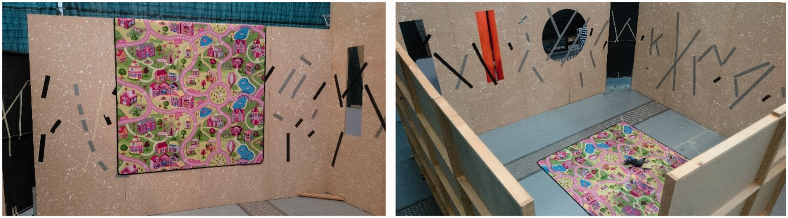
Two test flight rooms.

Results

Table 3 shows the summarized results obtained from the monocular test flights. Two main observations can be made from this table. First, the average number of stereo overrides during the test phase is 3, which is very close to the number of overrides in simulation. The monocular behavior also has a similar heat map to simulation. Figure 14 shows a heat map of the drone’s position during the approaches and the avoidance maneuvers (the turns). Again, the stereo-based flight performs better in the sense that the drone explores the room much more thoroughly and the turns happen consistently just before an obstacle is detected. On the other hand, especially in room 2, the monocular performance is quite good in the sense that the system is able to explore most of the room.

Figure 14.

Room 1 (plain texture) position heat map. Top row is the binned position during the avoidance turns, bottom row during the obstacle approaches, right column during stereo ground truth based operation, left column during learned monocular operation.

Table 3.

Test flight summary.

	Room 1					Room 2
Description	#1	#2	#3	#4	#5	#6	#7	#8	#9	#10	Avg.
Stereo flight time m:ss	6:48	7:53	2:13	3:30	4:45	4:39	4:56	5:12	4:58	5:01	4:59
Mono flight time m:ss	3:44	8:17	6:45	7:25	4:54	10:07	4:46	9:51	5:23	5:12	6:39
Mean square error	0.7	1.96	1.12	0.95	0.83	0.95	0.87	1.32	1.16	1.06	1.09
False positive rate	0.16	0.18	0.13	0.11	0.11	0.08	0.13	0.08	0.1	0.08	0.11
True positive rate	0.9	0.44	0.57	0.38	0.38	0.4	0.35	0.35	0.6	0.39	0.47
Stereo approaches	29	31	8	14	19	22	22	19	20	21	20.5
Mono approaches	10	21	20	25	14	33	15	28	18	15	19.9
Auto-overrides	0	6	2	2	1	5	2	7	3	2	3
Overrides ratio	0	0.72	0.3	0.27	0.2	0.49	0.42	0.71	0.56	0.38	0.41

Second, the selected TPR and FPR are on average 0.47 and 0.11. The TPR is rather low compared to the offline tests. However, this number is heavily influenced by the monocular estimator-based behavior. Due to the goal of the robot, avoiding obstacles slightly before the stereo ground truth recognizes them as positives, positives should hardly occur at al. Only in cases of FNs where the estimator is slower or wrong, positives will be registered by the ground truth. Similarly, the FPR is also lower in the context of the monocular-based behavior.

ROC curves of the 10 flights are shown in Figure 15. A comparison based on the numbers between the first five flights (room 1) and the last five flights (room 2) does not show any significant differences, leading to the suggestion that the system is able to learn both rooms equally well. However, when comparing the heat maps of the two situations in the monocular system in Figures 14 and 16, it seems that the system shows slightly different behavior. The monocular system appears to explore room 2 better, getting closer to copying the behavior of the stereo-based system. This is also pointed out by the peak in the heat map in the bottom row, left column of Figure 14; the binned position occurrence of the monocular behavior during the straights. It shows the behavior was affected by false positives, it sometimes turned too soon and too far from the walls, resulting in a peak in the middle of the room. Similarly, this is also visible when comparing the monocular turn locations (Figure 14, top row) to the stereo turn locations (Figure 14 top right). The stereo algorithm turns consistently close to the walls, while the monocular behavior shows a lot of spread and turns often quite far away from the walls. Interestingly, this problem partly disappears when more varied and natural texture is applied to the same room as shown by the results in Figure 16.

Figure 15.

Room 2 (carpet natural texture) position heat map. Top row is the binned position during the avoidance turns, bottom row during the obstacle approaches, right column during stereo ground truth based operation, left column during learned monocular operation.

Figure 16.

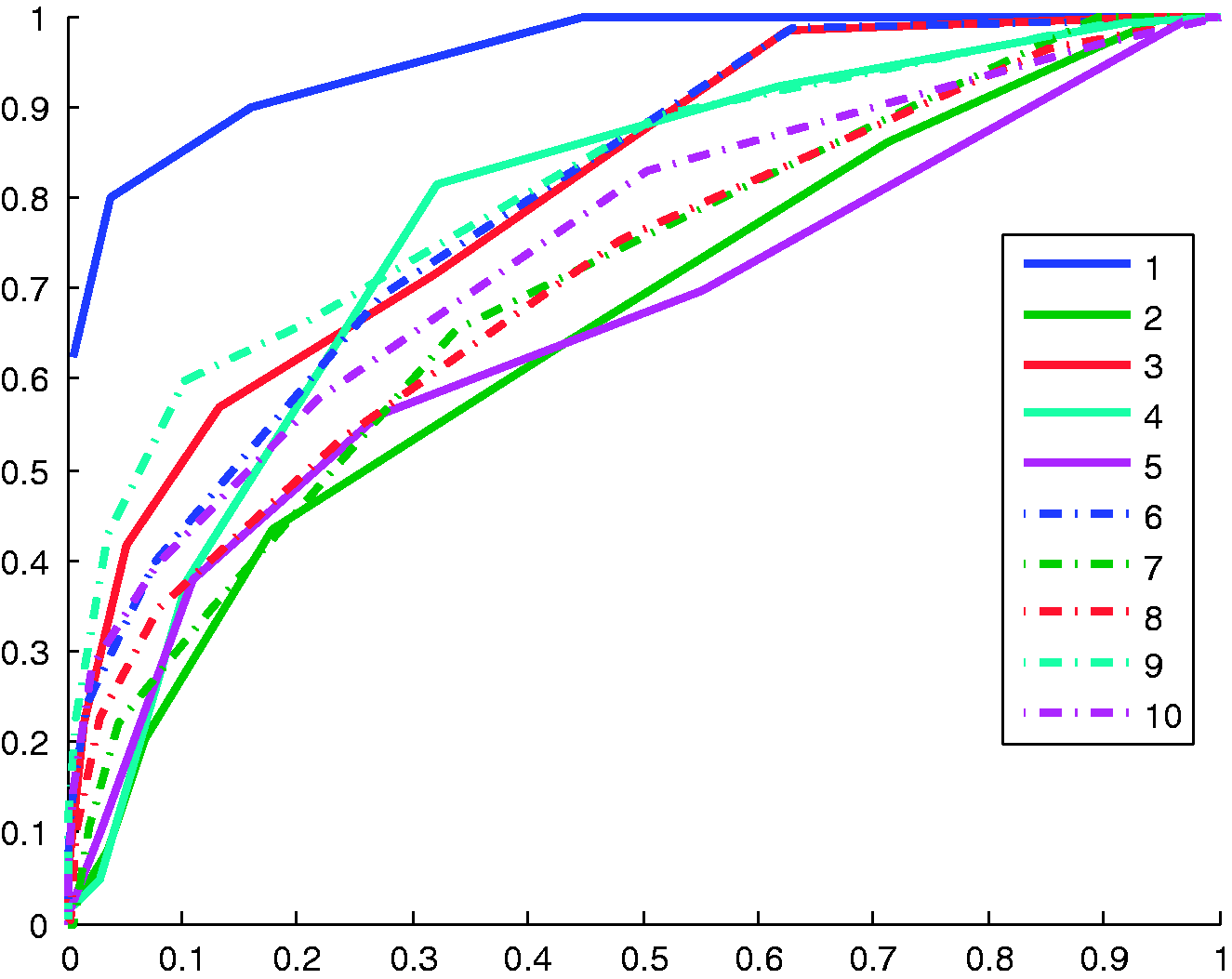
ROC curves of the 10 test flights. Dashed/solid lines refer to results on room #1/#2.

The experimental setup with the room in the motion tracking arena allows for a more in-depth analysis of the performance of both stereo and monocular vision. Figure 17 shows the spatial view of the flight trajectory of test #10 (note 2). The flight is segmented into approaches and turns which are numbered accordingly in these figures. The color scale in Figure 17(a) is created by calculating the theoretically visible closest wall based on the tracking the systems measured heading and position of the drone, the known position of the walls, and the FOV angle of the camera. It is clearly visible that the stereo ground truth in Figure 17(b) does not capture this theoretical disparity perfectly. Especially in the middle of the room, the disparity remains high compared to the theoretical ground truth due to noise in the stereo disparity map. The results of the monocular estimator in Figure 17(c) show another decrease in quality compared to the stereo ground truth.

Figure 17.

Flight path of test 10 in room 2. Monocular flight starts form approach 23. The meaning of the color of the flightpath differs per image; (a): the approximated disparity based on the external tracking system. (b): the measured stereo average disparity, (c): the monocular estimated disparity, (d): the error between the stereo disparity and monocular estimated disparity with dark blue meaning zero error, (e): error during FP, (f): error during FN. (e and f) only show the monocular part of the flight.

Discussion

We start the discussion with an interpretation of the results from the simulation and real-world experiments, after which we proceed by discussing persistent SSL in general and provide a comparison to other machine learning techniques.

Interpretation of the results

Using persistent SSL, we were able to autonomously navigate our multicopter on the basis of a stereo vision camera, while training a monocular estimator on board and online. Although the monocular estimator allows the drone to continue flying and avoiding obstacles, the performance during the approximately 10-min flights is not perfect. During monocular flight, a fairly limited amount of (autonomous) stereo overrides was needed while at the same time the robot was not fully exploring the room like when using stereo.

Several improvements can be suggested. First, we can simply have the drone learn for a longer time, accumulating training data over multiple flights. In an extended offline test, our VBoW method shows saturation at around 6000 samples. Using additional features and more advanced learning methods may result in improved performance if training set sizes increase.

During our tests in different environments, it proved unnecessary to tune the VBoW learning algorithm parameters to a new environment as similar performance was obtained. The learned results on the robot itself may or may not generalize to different environments; however, this is of less concern as the robot can detect a new environment and then decide to continue the learning process if the original cue is still available. In order to detect an inadequacy of the learned regression function, the robot can occasionally check the estimation error against the stereo ground truth. In fact our system already does so autonomously using its safety override. Methods on checking the performance without using the ground truth, e.g. by employing a learner that gives an estimate of uncertainty, are left for future work.

Deep learning

At the time of our robotic experiments, implementing state-of-the-art deep learning methods on-board a flying drone was deemed infeasible due to hardware restrictions. One of the major advantages of persistent SSL is the unprecedented amount of available training data. This amount of data will be more useful to more complex learning methods such as deep learning methods than to less complex, but computationally efficient methods such as the VBoW method used in our experiments. Today, with the availability of strongly improved hardware such as the NVidia Jetson TX1, close-to state-of-the-art models can be trained and run on-board a drone, which may significantly improve the learning results.

Persistent SSL in relation to other machine learning techniques

In order to place persistent SSL in the general framework of machine learning, we compare it with several techniques. An overview of this comparison is presented in Figure 18.

Figure 18.

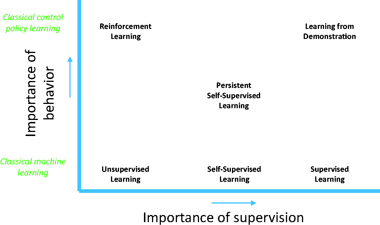
Lay of the machine learning land.

Un-/semi-/supervised learning

Unsupervised learning does not require labeled data, semi-supervised learning requires only an initial set of labeled data,⁴¹ and supervised learning requires all the data to be labeled. Internally, persistent SSL uses a standard supervised learning scheme, which greatly facilitates and speeds up learning. The typical downside of supervised learning—acquiring the labels—does not apply to SSL, since the robot continuously provides these labels itself.

A major difference between the typical use of supervised learning and its use in persistent SSL, is that the data for learning are generally assumed to be i.i.d. However, persistent SSL controls a behavioral component which, in turn, affects both the data set obtained during training as well as during testing time. Operation based on ground truth induces a certain behavior that differs significantly from behavior induced from a trained estimator, even more so for an undertrained estimator.

SSL

The persistent form of SSL is set apart in the figure from “normal” SSL, because the persistence property introduces a much more significant behavioral component to the learning. While normal SSL expects the trusted cue to remain available, persistent SSL assumes that the robot may sometimes act in the absence of the trusted cue. This introduces the feedback-induced data bias problem, which, as we have seen, requires specific behavior strategies for best learning the robot’s task.

Learning from demonstration

Imitation learning, or LfD, is a close relative to persistent SSL. Consider for instance teleoperation, an LfD scheme in which a (human or robot) teacher remotely operates a robot in order for it to learn demonstrated actions in its environment.²⁰ This can be compared to persistent SSL if we consider the teacher to be the ground truth function $g (x_{g})$ in the persistent SSL scheme. In most cases described in literature, the teacher shows actions from a control policy taken on the basis of a state instead of just the results from a sensory cue (i.e., the state). However, LfD does contain exceptions in which the learner only records the states during demonstration, e.g. when drawing a map through a 2D representation of the world in case of a path planning mission in an outdoor robot.⁴² Like persistent SSL, test time decisions taken in LfD schemes influence future observations which may or may not be contained in known demonstrated territory. However, one key difference between LfD and persistent SSL arguably sets them apart. All LfD theory known to the authors implicitly assumes the teacher is never the same entity as the learner. It may be that all relevant sensors are on the learner, and even that the learners body is used to execute teacher commands (like in teleoperation), but the teachers intelligence is always an external entity.

Reinforcement learning

Lastly, we compare persistent SSL with RL, which is a distinctively different technique.⁴³ In RL, a policy is learned using a reward function. Due to the evaluative feedback provided in RL, defining a good reward function is one of fundamental difficulties of RL known as reward shaping.^43,44 Since persistent SSL uses supervised feedback, reward shaping is less of an issue in persistent SSL, only requiring a choice of a loss function between $g (x_{g})$ and $f (x_{f})$ . Secondly, the initial exploration phase of RL often infers a lot of trial-and-error, making it a dangerous time in which a physical system may crash and be damaged. Although this particular problem is often solved by better initialization, e.g. by using for instance LfD or using policy search instead of value function-based approaches, persistent SSL does not require an untrained initialization phase at all as a reliable ground truth function guarantees a certain minimal correct behavior.

Persistent SSL differs from other learning techniques in the sense that no complete training data set is needed to train the algorithm beforehand. Instead it requires a ground truth $g (x_{g})$ , which must be available online in real time while training $\hat{f} (x_{f})$ , but can be switched off when $\hat{f} (x_{f})$ is learned to satisfaction. This implies that learning needs to be persistent and that the switch θ must be included in the model. Note that in cases where the environment of the robot may change, measures can be put in place to detect the output uncertainty of $\hat{f} (x_{f})$ . If the uncertainty goes up, the robot can switch back to using the ground truth function and learning can then be activated again. Developing such measures is, however, left for future work.

Feedback-induced data bias

The robot induces how its environment is perceived, meaning it influences the acquired training samples based on its behavior. The problems arising from this feedback-induced data bias are known from other machine-learning disciplines, such as RL and LfD.⁴³ In particular, Ross et al. have proposed DAgger² to solve a similar problem in the LfD domain, which iteratively aggregates the data set with induced training samples and the experts reaction to it. However, in the case of LfD, obtaining the induced training samples requires a careful engineered and often additional setup, while in persistent SSL, this functionality is inherently available. Secondly, the performance of the LfD expert (i.e., in many cases, a human) is not easy to control, often reacting too late or too early. The control policy of the persistent SSL ground truth override system can, on the other hand, be very deterministic. In the case of a DAgger application with drones flying through a forest,³ it proved infeasible to reliably sample the expert in an online fashion. Acquired videos had to be processed offline by the expert, hence the need for (offline ↔ online) iterations. Moreover an additional online human safety override interface was still necessary to prevent damage to the drone while learning. Thirdly, due to the cost of (and need for) iterative demonstration sessions, the emphasis of DAgger is on converging fast with needing as little expert sessions as possible. In persistent SSL, there are no costs for using the teacher signals coming from the original sensor cue. With persistent SSL, we can directly focus on effectively using the available amount of training samples instead of minimizing the number of iterations like in DAgger.

Another reason why persistent SSL handles the induced training sample issue better than other state of the art robot learning methods, is that in persistent SSL part of the learning problem itself can be easily separated and tested from the behavior; i.e. in a traditional supervised learning setting. In our proof of concept, this has allowed us to test the learning algorithms and thoroughly investigate its limits before deployment.

Conclusion

We have investigated the behavioral aspects of an SSL scheme, in which the supervisory signal is switched off after an initial learning period. In particular, we have studied an instance of such “persistent SSL” for the task of obstacle avoidance, in which the robot uses trusted stereo vision distance estimates in order to learn appearance-based monocular distance estimation. We have shown that this particular setup is very similar to LfD. This similarity has been corroborated by experiments in simulation, which showed that the worst learning strategy is to make a hard switch from stereo vision flight to mono vision flight. It is best to have the robot fly based on mono vision and using stereo vision only as “training wheels,” to take over when the robot would otherwise collide with an obstacle. The real-world robot experiments show the feasibility of the approach, giving acceptable results already with just 4–5 min of learning.

The findings also indicate interesting future venues of investigation. First, and perhaps most importantly, in the 4–5 min of the real-world experiments, the robot already experiences roughly 7000–9000 supervised learning samples. It is clear that longer learning times can lead to very large supervised data sets, which are suitable for deep learning approaches. Such approaches likely allow the learning to extend to much larger and more varied environments, such as outdoor forests or multiple rooms inside larger buildings. In addition, they could allow the learning to improve the resolution of disparity estimates from a single value to a full image size disparity map. Second, in the current experiments, the robot stayed in a single environment. We mentioned that a different environment can make the learned mapping invalid, and that this can be detected by means of the ground truth. Another venue, as studied in Ho et al.,¹² is to use a machine learning method with an associated uncertainty value. For instance, one could obtain uncertainty estimates by using a learning method such as a Gaussian Process or by using dropout with deep neural networks. This can help with a further integration of the behavior with learning, for instance by tuning the forward velocity based on the certainty. These venues together could allow for persistent SSL to reach its full potential, significantly enhancing the robustness of robots operating in real-world environments.

Footnotes

Declaration of conflicting interests

The author(s) declared no potential conflicts of interest with respect to the research, authorship, and/or publication of this article.

Funding

The author(s) received no financial support for the research, authorship, and/or publication of this article.

Notes

References

García

and Fernández

A comprehensive survey on safe reinforcement learning. J Mach Learn Res 2015; 16: 1437–1480.

Ross

Gordon

and Bagnell

JA.

A reduction of imitation learning and structured prediction. In: 14th International conference on artificial intelligence and statistics, Ft. Lauderdale, FL, USA, p. 15, 2011.

Ross

Melik-Barkhudarov

Shankar

et al . Learning monocular reactive UAV control in cluttered natural environments. In: 2013 IEEE international conference on robotics and automation, Karlsruhe, Germany, pp. 1765–1772, 2013.

Thrun

Montemerlo

Dahlkamp

et al . Stanley: the robot that won the darpa grand challenge. In: The 2005 DARPA grand challenge, pp. 1–43. Springer, 2007.

Lieb

Lookingbill

and Thrun

Adaptive road following using self-supervised learning and reverse optical flow. In: Sebastian T, Gaurav S. Sukhatme and Stefan S (eds.) Robotics: science and systems, 2005, MIT Press, Cambridge, Massachusetts, pp. 273–280.

Lookingbill

Rogers

Lieb

et al . Reverse optical flow for self-supervised adaptive autonomous robot navigation. Int J Comp Vision 2007; 74: 287–302.

Procopio

Mulligan

and Grudic

Learning terrain segmentation with classifier ensembles for autonomous robot navigation in unstructured environments.

J Field Robot 2009; 26: 145–175.

Bajracharya

Howard

Matthies

et al

Autonomous off-road navigation with end-to-end learning for the lagr program.

J Field Robot 2009; 26: 3–25.

Hadsell

Sermanet

Ben

et al

Learning long-range vision for autonomous off-road driving.

J Field Robot 2009; 26: 120–144.

10.

Muller

, Jackel

, LeCun

et al . Real-time adaptive off-road vehicle navigation and terrain classification. In: SPIE defense, security, and sensing, pp. 87410A–87410A. San Diego, California United States: International Society for Optics and Photonics, 2013.

11.

Baleia

Santana

and Barata

On exploiting haptic cues for self-supervised learning of depth-based robot navigation affordances. J Intellig Robot Syst 2015; 80(3-4): 455–474.

12.

De Wagter

Remes

BDW

et al . Optical flow for self-supervised learning of obstacle appearance. In: Intelligent robots and systems (IROS), 2015 IEEE/RSJ international conference, pp. 3098–3104. IEEE, September 28 - October 2, 2015, Congress Centre Hamburg, Hamburg, Germany.

13.

Lamers

Tijmons

De Wagter

et al . Self-supervised monocular distance learning on a lightweight micro air vehicle. In: Intelligent robots and systems (IROS), 2016 IEEE/RSJ international conference, Daejeon, Korea, October 9-14, 2016, pp. 1779–1784. IEEE, 2016.

14.

Gandhi

Pinto

and Gupta

Learning to fly by crashing. arXiv preprint arXiv:1704.05588, 2017.

15.

Mori

and Scherer

First results in detecting and avoiding frontal obstacles from a monocular camera for micro unmanned aerial vehicles. In: Proceedings—IEEE international conference on robotics and automation, Karlsruhe, Germany, pp. 1750–1757, 2013.

16.

Engel

Sturm

and Cremers

Scale-aware navigation of a low-cost quadrocopter with a monocular camera.

Robot Autonom Syst 2014; 62: 1646–1656.

17.

van Breugel

Morgansen

and Dickinson

MH.

Monocular distance estimation from optic flow during active landing maneuvers.

Bioinspirat Biomimet 2014; 9: 025002.

18.

de Croon

GCHE.

Monocular distance estimation with optical flow maneuvers and efference copies: a stability-based strategy.

Bioinspirat Biomimet 2016; 11: 016004.

19.

de Croon

GCHE

Groen

De Wagter

et al . Design, aerodynamics and autonomy of the DelFly. Bioinspirat Biomimet 2012; 7: 025003.

20.

Argall

Chernova

Veloso

et al . A survey of robot learning from demonstration. Robot Autonom Syst 2009; 57: 469–483.

21.

Guo

Lee

Wang

et al

. Deep learning for real-time Atari game play using offline Monte Carlo tree search planning. In: Proceedings of conference on neural information processing systems (NIPS), vol. 2600, Montréal, Canada, pp. 1–9, 2014.

22.

Sadeghi F and Levine S. (cad)2rl: real single-image flight without a single real image. arXiv preprint arXiv:1611.04201, 2016.

23.

Hoiem

Efros

and Hebert

Automatic photo pop-up.

ACM Trans Graph 2005; 24: 577.

24.

Saxena

Chung

and Ng

AY.

3-D depth reconstruction from a single still image.

Int J Comput Vis 2007; 76: 53–69.

25.

Saxena

Sun

and Ng

AY.

Make3D: learning 3D scene structure from a single still image. IEEE Trans Pattern Anal Mach Intellig 2009; 31: 824–840.

26.

Lenz

Gemici

and Saxena

Low-power parallel algorithms for single image based obstacle avoidance in aerial robots. In: IEEE international conference on intelligent robots and systems, Vilamoura, Algarve, Portugal, pp. 772–779, 2012.

27.

Eigen

Puhrsch

and Fergus

Depth map prediction from a single image using a multi-scale deep network. In: Advances in neural information processing systems, (NIPS 2014), Montréal, Canada, pp. 1–9, 2014.

28.

Michels

Saxena

and Ng

AY.

High speed obstacle avoidance using monocular vision and reinforcement learning. In: Proceedings of the 22nd international conference on machine learning, vol. 3, Bonn, Germany, August 07 - 11, 2005, pp. 593–600. ACM Press, 2005.

29.

Dey

Shankar

Zeng

et al . Vision and learning for deliberative monocular cluttered flight, pp.391-409. Springer, 2016.

30.

Yamauchi

Oota

and Ishii

A self-supervised learning system for pattern recognition by sensory integration.

Neural Netw 1999; 12: 1347–1358.

31.

Thrun

Montemerlo

Dahlkamp

et al . Stanley: the robot that won the DARPA grand challenge. Springer Tracts Adv Robot 2007; 36: 1–43.

32.

De Wagter

Tijmons

Remes

BDW

et al

. Autonomous flight of a 20-gram flapping wing MAV with a 4-gram onboard stereo vision system. In: IEEE international conference on robotics & automation (ICRA), number Section IV, 31 May - 07 Jun 2014, Hong Kong, China, pp. 4982–4987, 2014.

33.

De Croon

GCHE

De Weerdt

De Wagter

et al . The appearance variation cue for obstacle avoidance. IEEE Trans Robot 2012; 28: 529–534.

34.

Varma

and Zisserman

Texture classification: are filter banks necessary? 1 Introduction 2 A review of the VZ classifier. In: Computer vision and pattern recognition 2003 proceedings 2003 IEEE computer society conference, 2003, Madison, Wisconsin June 16-22, 2003.

35.

Ooi

and He

ZJ.

Perceiving distance accurately by a directional process of integrating ground information.

Nature 2004; 428: 73–77.

36.

van Hecke

Monocular obstacle avoidance with persistent self-supervised learning dataset. data.4TU.nl, 2017, Available at https://doi.org/10.4121/uuid:a3599d11-d56a-4402-93f8-2e7c22cf5dab

37.

De Wagter

and Amelink

MHJ.

Development of inertial navigation, onboard vision and adaptive control for autonomous long-distance mav operations. In: Conference: European micro air vehicle conference and competittion, Toulouse, France, 2007.

38.

Cohen

PR.

Empirical methods for artificial intelligence. IEEE Intellig Syst 1996; (6): 88.

39.

B.D.W. Remes, Dino Hensen, Freek Van Tienen, Christophe De Wagter, Erik Van der Horst, and G.C.H.E. De Croon. Paparazzi: how to make a swarm of parrot AR drones fly autonomously based on GPS. In: IMAV 2013: proceedings of the international micro air vehicle conference and flight competition, Toulouse, France, 17–20 September 2013.

40.

Brisset

Drouin

Gorraz

et al . The Paparazzi solution, MAV 2006, 2nd US-European Competition and Workshop on Micro Air Vehicles, Oct 2006, Sandestin, United States.

41.

Zhu

Semi-supervised learning literature survey. Sciences-New York, 2007, pp. 1–59 (1530). Computer Sciences, University of Wisconsin-Madison.

42.

Ratliff

Bradley

Bagnell

et al . Boosting structured prediction for imitation learning for imitation learning. In: Advances in neural information processing systems (NIPS), 2006, Vancouver, B.C., Canada, p. 54.

43.

Kober

Bagnell

and Peters

Reinforcement learning in robotics: a survey. Int J Robot Res 2013; 32: 1238–1274.

44.

Littman

ML.

Reinforcement learning improves behaviour from evaluative feedback.

Nature 2015; 521: 445–451.

Persistent self-supervised learning: From stereo to monocular vision for obstacle avoidance

Abstract

Keywords

Introduction

Related work

Monocular navigation

Appearance-based navigation without distance estimation

Offline monocular distance learning

Self-supervised learning

Methodology overview

Persistent SSL principle

Stereo-to-mono proof of concept

Stereo vision processing

Monocular disparity estimation

Control behavior

Performance

Similarity with LfD

Learning schemes

Offline vision experiments

Simulation experiments

Setup

Results

Robotic experiments

Results

Discussion

Interpretation of the results

Deep learning

Persistent SSL in relation to other machine learning techniques

Un-/semi-/supervised learning

SSL

Learning from demonstration

Reinforcement learning

Feedback-induced data bias

Conclusion

Footnotes

Declaration of conflicting interests

Funding

Notes

References