Sage Journals: Discover world-class research

Abstract

An advanced driving assistant system is one of the most popular topics nowadays, and depth estimation is an important cue for advanced driving assistant system. Depth prediction is a key problem in understanding the geometry of a road scene for advanced driving assistant system. In comparison to other depth estimation methods using stereo depth perception, determining depth relation using a monocular camera is considerably challenging. In this article, a fully convolutional neural network with skip connection based on a monocular video sequence is proposed. With the integration framework that combines skip connection, fully convolutional network and the consistency between consecutive frames of the input sequence, high-resolution depth maps are obtained with lightweight network training and fewer computations. The proposed method models depth estimation as a regression problem and trains the proposed network using a scale invariance optimization based on L2 loss function, which measures the relationships between points in the consecutive frames. The proposed method can be used for depth estimation of a road scene without the need for any extra information or geometric priors. Experiments on road scene data sets demonstrate that the proposed approach outperforms previous methods for monocular depth estimation in dynamic scenes. Compared with the currently proposed method, our method has achieved good results when using the Eigen split evaluation method. The obvious prominent one is that the linear root mean squared error result is 3.462 and the δ < 1.25 result is 0.892.

Keywords

Depth estimation monocular sequence fully convolutional neural network road scene

Introduction

Estimating depth from a single image is a very important problem in the computer vision field. In general, depth estimation is a key problem for many research topics such as three-dimensional (3-D) modeling, 3-D reconstruction, scene understanding, object detection and robotics, semantic segmentation, human activity recognition, and so on.

Most of the depth estimation methods predict depth from stereo images and achieved good performances. Stereo methods rely on stereo images captured from multiple cameras to ensure that the problem of depth prediction is well-posed, where depths are estimated using geometrical computations,¹ additional sensors,² and photometric or consistency checks.³ Although the stereo image method can obtain relatively accurate scene depth information, the depth result tends to be sparse. Furthermore, the estimated depth tends to be inaccurate when the distances considered are large, and a small matching error often causes a large depth estimation error.

Because of the ill-pose problem, estimate depth from a single image is much more challenging than depth estimation from stereo images. Previous studies using single image techniques focus on scene-dependent knowledge, for example, “Blocks World” model,⁴ shape from shading,⁵ and shape from the silhouette. Among these monocular methods, structure-from-motion (SfM)⁶ is the most successful one. It predicts depth with multiple images captured from a single camera at different time intervals. That is, it estimates camera translation between sequence image pairs by different temporal intervals, and then, estimate depth through camera motion. However, these models typically work for images with particular scenes structures, and therefore, they are not applicable to road scene depth estimations.

A method suggested by Saxena et al.⁷ considers each super-pixel extracted from the image as a plane with the same depth, and then infers the construction parameters of the super-pixel plane using a Markov random field (MRFs) to obtain the depth. In addition, the methods in the literature studies^8
–10 regard super-pixels as a plane of the same depth, and they estimate depth using the conditional random field (CRF). More recently, a data-driven method is often used to estimate the depth from the image, such as Karsch et al.^11,12 and Konrad et al.¹³ These methods match image features with the RGBD data set and predict depth by exploiting the relationship between the image features and the depth. However, these methods use handcrafted features, which result in low accuracy.

In recent years, the monocular image depth estimation method based on convolutional neural networks (CNNs) has achieved considerable success. Most studies initialize their networks with AlexNet¹⁴ or visual geometry group (VGG),¹⁵ and then, optimize network parameters according to their requirements and data set. Eigen et al.¹⁶ first proposed a solution for image depth estimation using CNNs. They estimate depth from a concise network with the photometric error between output and ground truth as loss function and pre-train the convolutional layers of the coarse-scale network on ImageNet. Eigen and Fergus¹⁷ later extend their work and develop a well-designed network that uses three scales of inputs to generate the more general features and refine predictions to higher resolutions, including surface normal estimation and per-pixel semantic labeling.

Unlike the above two methods, Roy and Todorovic¹⁸ combine CNN with Regression Forest for predicting depths in the continuous domain via regression. At every tree node, they filter the sample with a CNN associated with that nod and design CNN at every node of convolutional regression trees (CRTs) to obtain significantly fewer parameters. That, in turn, allows for robust training on a smaller data set. Also, some methods often combine CNN with CRFs or MRFs to achieve the post-processing of depth estimation and optimize the estimation results of deep networks. Liu et al.¹⁹ consider the continuous characteristic of the depth values formulated into a CRF learning problem. In particular, they use an end-to-end deep CNN network to learn the pairwise potentials of CRF with a deeply designed learning pipeline. Li et al.⁸ use the CRF to optimize the super-pixel-level depth estimation results obtained by CNNs. Wang et al.¹⁰ then proposed a method that predicts depth and semantic jointly. They first use a pre-trained CNN model to estimate the pixel-level depth and semantic labels. Then, they decompose the input image into segments to achieve further pixel-level results. By formulating the depth estimate and semantic problem into a hierarchical CRF, they achieve state-of-art results. Kim et al.²⁰ present a method for jointly predicting a depth map and intrinsic images from single-image input using a novel CNN architecture. The model includes a depth and intrinsic prediction network, a gradient scale network, and a joint CRF. The method in the literature²¹ has also achieved good results by designing a new CNN implementation where training can be performed end-to-end. Compared with other methods, the image depth estimation method based on CNN learning can achieve better real-time performances and consequently obtain better accuracy. The method in the literature²² treats the depth estimate as a multi-class classic problem and achieves a good depth estimation effect through a well-designed network.

Recently, the fully convolutional network (FCN) has achieved good results in object detection,^23,24 semantic segmentation,^25

–28 and depth estimation.^29,30 The skip connection structure used in FCN has been proven to merged the coarse and abstract information in different layers, this helps to extract the feature information of the input while making the output image the same size as the input image. Inspired by that, we use skip connection structure to learn the feature extraction in depth estimation problem and output pixel-level depth image. The methods in the literature studies^31,32 also use the FCN network structure for depth estimation, but the depth estimation part and pose estimation part of their network are separated. In their method, the deep estimation network part uses a single picture as input, and pose estimation network uses the front and back frame image of sequence or image pairs as input.

In this article, we are concerned with the challenge of monocular-based depth estimation. A fully CNN with skip connection based on a monocular video sequence is proposed to estimate depth. The network takes two neighboring images in a monocular video sequence as input and output pixel-level images. Skip connection and multi-layer deconvolution networks are used to preserve more information and output pixel-level results. With the integration framework that combines skip connection, FCN network and the consistency between consecutive frames of the input sequence, high-resolution depth maps are obtained with lightweight network training and fewer computations. The proposed method models depth estimation as a regression problem and trains the proposed network using a scale invariance optimization based on L2 loss function, which measures the relationships between points in the consecutive frames. The proposed method can be used for depth estimation of a road scene without the need for any extra information or geometric priors. Our network implicitly learns the pose relationship between the input images, which is conducive to the accuracy of the depth estimations results, and our method achieved good results on the KITTI data set.

The remainder of this article is organized as follows. Section “Network architecture” describes the details of our network architecture (subsection “Architecture”) and loss function (subsection “Loss function”) for depth estimation, and in section “Experiments,” the experimental setup (subsection “Experimental setup”), the evaluation metrics (subsection “Evaluation metrics”), the parameters settings (subsection “Experimental parameters”), and the experimental results (subsection “Experimental results”) are introduced. We conclude the article in the “Conclusion” section.

Network architecture

Architecture

Our purpose is to estimate the depth map corresponding to the road scene picture. Because of the ill-pose problem of a single picture, most methods now use additional information to constrain depth, such as optical flow information, CRF, motion information, and so on. Our method uses motion information, takes two pictures I and I ⁻¹ as input, and outputs a pixel-level depth map of single image I, where I and I ⁻¹ represent to two adjacent frames of the video sequence.

Inspired by the methods in literature studies,^16,33 we treat the depth estimation problem as a supervision problem. In other words, we have the picture of scenes and the corresponding ground truth of the scene during training. However, most monocular supervision methods take a single picture as input and have ill-pose problems and do not use important hidden information in the road scene video sequence. As shown in Figure 1, Eigen et al.¹⁶ and Xu et al.²¹ only take the single image as input and do not take advantage of the feature information of multiple images. We solve this problem by supervising the depth of prediction by taking two images I and I ⁻¹ as the input to the network.

Figure 1.

Sampling strategies for feature extraction. Eigen et al. use the classic CNN network structure and Xu et al. and our method use the FCN network structure. Eigen et al. and Xu et al. use single image as input, while our method takes two images as input. CNN: convolutional neural network; FCN: fully convolutional network.

Our FCN is inspired by FCN in the literature studies,^17,34 but we doubled the number of input layers to accommodate the doubling of the number of input images and made some modifications to accommodate the depth estimation instead of the semantic segmentation. As shown in Figure 2, different from the Kuznietsov et al.³⁵ and SfM-net,³⁶ we use an FCN to simultaneously predict the depth and obtain motion implicitly. And Kuznietsov et al.³⁵ use binocular images as input and additional binocular targeting information as supervision, while we use the front and back frames as input. Unlike SfM-net,³⁶ because we treat depth estimation as supervised learning, we do not have a pose network part, which means we have fewer network parameters and shorter training time.

Figure 2.

Sampling strategies for image inputs. Different from Kuznietsov et al.³⁵ and SfM-net,³⁶ we treat depth estimation as supervised learning, and our pipeline is more concise as we do not require additional pose information.

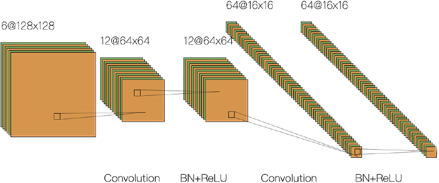
The proposed network architecture is illustrated in Figure 3. The network architecture consists of two parts: a convolution (encoder) part and a deconvolution (decoder) part.

Figure 3.

Network architecture.

The convolution part takes two consecutive frames of a video sequence as input, and it uses the global view of the input scene to predict the structure of the overall depth map. It follows the typical architecture of a convolutional network. To accommodate twice the amount of input, we set the first layer of the conventional part as six channels, and the subsequent convolution layers are modified accordingly to fit the number of channels of the first layer. Further, the conventional part consists of repeated applications of unpadded convolutions. Each layer of the convolution part is a convolution block. To get better features, different convolution blocks use different filters for the input image to select relevant feature representations. Rectified Linear Units (ReLUs) are used as an activation function for the convolution block, and max-pooling layers are performed between these convolutional blocks to encode the global information. The number of features in the first convolution layer of each convolution block is twice the number of features in the last convolution layer of the upper layer convolution block. Specifically, the size of the first convolutional layer in each convolution block is half the size of the input layer before downsampling. Suppose the input size is $h_{i} * w_{i}$ . The size of the convolutional layer after downsampling is $h_{o} * w_{o}$ with stride s. The length and width of the output convolutional layer are expressed as $h_{o} = [\frac{h_{i}}{s}]$ and $w_{o} = [\frac{w_{i}}{s}]$ , respectively. The structure in each convolution block is shown in Figure 4. And the convolutional layer is obtained by convolving the previous convolutional layer and performing a modified linear activation of the ReLU. Also, max-pooling operations are not performed in inner layers to restore the spatial information of features.

Figure 4.

Convolution structure in the convolution block.

The deconvolution part results in an output image containing the depth of each pixel. Each layer of the deconvolution part includes several deconvolution layers, and each deconvolution layer contains two parts: upsampling layer obtained by upsampling the feature map through deconvolution and feature layer obtained by concatenating the corresponding feature map from the convolution part. The skip connection is added so that the information of the convolution layer is merged into the feature layer. The advantage is that more image information is integrated during the learning process of the upsampling parameter, thereby improving the accuracy of the learning of the upsampling parameter. And the final output of the deconvolution part is the depth information of each pixel of the input image.

During training, the network architecture consists of five convolutional blocks and five deconvolution layers. Specifically, the first two convolution blocks contain two convolutional layers, and the last three convolutional blocks contain three convolutional layers. The convolution kernel size in all five convolutional blocks is 3 * 3, and the convolution kernel of the convolutional layer in each convolution block is the same as the convolution kernel of the convolutional block. It should be noted that the size of the convolution kernel refers to the settings of other networks, such as Res-Net. It can be seen from another article that this parameter is a better parameter selected and is an empirical value. During the experiment, we also tried to use a 5 * 5 convolution kernel instead of a 3 * 3 convolution kernel, but the effect became worse. We think that the possible reason is that the size of different objects in the road scene dataset is quite different, and the 3 * 3 convolution kernel may have better feature extraction results.

A three-layer convolution connection layer is performed between the convolution part and the deconvolution part. The convolution kernel size used in the convolution connection layer is 1 * 1 to unify the channel of features. ReLU is used as activation functions for the convolution layer. At the same time, to prevent overfitting the model, a dropout is applied after the first two convolution connection layers.

Loss function

The conventional method of image depth estimation based on deep learning is often used to consider depth estimation as a classification problem, and the image depth value is treated as a category label or the super-pixels in the image. Then the CRF is used to further optimize the depth value of the pixels in each super-pixel or block. However, if each pixel in the image is directly subjected to deep estimation based on FCN deep learning, the depth estimation problem can be regarded as a regression problem, which can make the loss function simpler. A standard loss function for optimization in regression problems is the L2 loss function, which often achieves good results. Our method performs scale invariance optimization based on the standard L2 loss function. Suppose y and $\tilde{y}$ represent the ground truth value and the predicted depth value. Then, the loss function can be defined as

L (y, \tilde{y}) = \sum_{i} d_{i}^{2} - \frac{λ}{n^{2}} {(\sum_{i} d_{i})}^{2}

where $d_{i}^{2} = ‖y_{i} - {\tilde{y}}_{i}‖$ represents the L2 distance between the ith pixel of the real depth image and the ith pixel of the predicted depth image. $λ \in [0, 1]$ is used to balance the relationship between the two items, n is the number of valid points in the image. We set $λ = 0.5$ as the balance between L2 loss and scale-invariant optimization loss. This parameter is a hyper-parameter and is set according to experience. As given in Table 1, the appropriate parameter results in good absolute-scale predictions while slightly improving qualitative output, and the inappropriate parameter will make some of the indicators in the result worse.

Table 1.

λ parameter setting.

	Threshold $δ < 1.25$	Threshold $δ < {1.25}^{2}$	Threshold $δ < {1.25}^{3}$	Rel	Linear RMSE	Log RMSE
$λ = 0.1$	0.850	0.820	0.976	0.122	4.280	0.227
$λ = 0.9$	0.882	0.897	0.967	0.127	4.870	0.253
$λ = 0.5$	0.892	0.970	0.988	0.119	3.462	0.162

Rel: Abs relative difference; Linear RMSE: linear root mean squared error; Log RMSE: log root mean squared error.

During the training process, there are many pixel points with insufficient depth information or nonexistence in the target depth map, especially at the target edge, window, or smooth surface. These points are filtered out and only the valid points are used to calculate the loss function.

Experiments

In this section, we introduce the training and test data sets, the parameters during the training process, and the evaluation criteria of the prediction results. We train our model on the raw versions KITTI,³⁷ which is an open outdoor scenes data set. The binocular video sequence is used from the data set. During the training process, left and right image data are used as training samples respectively to increase the number of training images. Note that the left and right sequences in the binocular are only regarded as monocular video sequences of the road scene during the training process, and the left and right sequences are completely independent and do not affect each other. The reason for using the left and right sequences as the training data set is merely to increase the number and diversity of training samples.

Experimental setup

KITTI data set

The KITTI data set³⁷ is a widely used road scene data set, and it consists of a variety of outdoor scene pictures obtained from a binocular camera and ground truth obtained from radar sensor. To be able to perform comparison experiments fairly, we use the same training data and test data used by Eigen et al.,¹⁶ that is, 39,810 images for train and 4424 images for test split from 58 scenes from “City,” “Residential,” and “Road” categories.

Because the depth of the KITTI data set is obtained at different times using a rotating radar scanner. Therefore, there may be large errors in the ground truth depth used for training. We choose the average depth of the closest pixels to eliminate larger error pixels. Besides, radar only provides ground truth measures for the lower half of the scene. And to compare the fairness of the experiment, we use the same training set data processing method as Eigen et al.,¹⁶ we use the bottom part of the image as input to train our model. The output prediction results are only tested for the bottom half of the input test image.

Data augmentation

The training data were augmented with random online transformations to make the data set have more variability. For the data sets used in this study, the main data set expansions include:

Rotation: Training images and ground truth are rotated by $r \in [- 5, 5]$ degrees,

Color: RGB channels of training images are scaled globally by a random value $c \in [0.8, 1.2]$ , and

Flips: Training images and ground truth images are flipped with 0.5 probability.

The rotation of the image can overcome the jitter of the image during the shooting to some extent. The change in color can reflect the evolution of illumination, which can reduce the precision of the prediction result. The flips of images are geometry-preserving, which can increase the diversity of training data.

Note that all data augmentation operations are performed for the two consecutive frames input into the system. In other words, the transformation of the input current frame and the consecutive previous frame is the same. Also, during data augmentation, the geometric space of the dataset is unchanged, and the coordinate system is stable. During the test, no transformation is performed on the input image.

Evaluation metrics

We compared our proposed approach with other state-of-the-art single-camera depth estimation methods. The comparison method was evaluated by the Accuracy with threshold thr (ACC), Abs relative difference (Rel), linear root mean squared error (Linear RMSE), and log root mean squared error (Log RMSE). The benchmark metrics for our comparisons are:

Accuracy with threshold $δ : max (\frac{y_{i}}{{\tilde{y}}_{i}}, \frac{{\tilde{y}}_{i}}{y_{i}}) = δ < thr$

Abs relative difference: $\frac{1}{| T |} \sum_{y \in T} | y_{i} - {\tilde{y}}_{i} | / {\tilde{y}}_{i}$

RMSE (linear): $\sqrt{\frac{1}{| T |} \sum_{y \in T} {‖y_{i} - {\tilde{y}}_{i}‖}^{2}}$

RMSE (log, scale-invariant): $\sqrt{\frac{1}{| T |} \sum_{y \in T} {‖log y_{i} - log {\tilde{y}}_{i}‖}^{2}}$

where y and

\tilde{y}

represent the true depth value and the predicted depth value, and T is the total number of effective pixel points.

Experimental parameters

We train our model using a single Nvidia GTX K40c GPU. The network parameters are initialized with random initialization. Specifically, we use 39,810 images of the KITTI data set for train and 4424 images as validation items and train our model using stochastic gradient descent (SGD) with a batch size of 12. The learning rate is set to 0.001 at the first 10 epochs and change to 0.0001 at the next 20 epochs. Because there is no additional re-projection process and pose-CNN or the process of generating super-pixels to obtain other information, our training time rarely takes only about 15 h. During the test, we can get the depth map of the input image in about 0.1 s.

In the training process, the input data is downsampled, and half of the size of the original image data is used as the input of the network structure. Furthermore, as the image size in the KITTI data set is 344 * 1152, and only the lower half of the image is used as the training sample so that the input image size is 86 * 576.

The FCN model is divided into a convolution part and a deconvolution part. The convolution part includes five convolution blocks and three convolution connection layers. Each convolution block is followed by a max-pooling layer; there is no max-polling layer between convolution layers in the same convolution block. The input of the convolution part is two consecutive frames with RGB channels, and the two images have a total of six channels. In our method, the stereo relationship in the left and right images is not required, and therefore, depth estimation can be completed only using the monocular image sequence. The deconvolution part consists of five layers of deconvolution. Each deconvolution layer is an upsampling process. The final output is the depth estimate of the gray channel, and some parameters of the convolution part of the deep network are set as listed in Tables 2 and 3; the parameters of the deconvolution part are listed in Table 4.

Table 2.

Convolution part parameter setting.

Convolution part
L	Conv1		Conv2		Conv3			Conv4			Conv5
L	1–1	1–2	2–1	2–2	3–1	3–2	3–3	4–1	4–2	4–3	5–1	5–2	5–3
K	3	3	3	3	3	3	3	3	3	3	3	3	3
s	1	2	1	2	1	1	2	1	1	2	1	1	2
i_chns	6	64	64	128	128	256	256	256	384	384	384	512	512
o_chns	64	64	128	128	256	256	256	384	384	384	512	512	512
i_size	86/576	86/576	43/288	43/288	22/144	22/144	22/144	11/72	11/72	11/72	6/36	6/36	6/36
o_size	86/576	43/288	43/288	22/144	22/144	22/144	11/72	11/72	11/72	6/36	6/36	6/36	3/18
Ratio	1	1/2	1/2	1/4	1/4	1/4	1/8	1/8	1/8	1/16	1/16	1/16	1/32
Input	im	1–1	1–2	2–1	2–2	3–1	3–2	3–3	4–1	4–2	4–3	5–1	5–2

Table 3.

Convolution connection part parameter setting.

Convolution connection part
L	Conv_fc1	Conv_fc2	Conv_fc3
K	1	1	1
S	1	1	1
i_chns	512	4096	4096
o_chns	4096	4096	1024
i_size	3/18	3/18	3/18
o_size	3/18	3/18	3/18
Ratio	1/32	1/32	1/32
Input	Conv5–3	Conv_fc1	Conv_fc2

Table 4.

Deconvolution part parameter setting.

Deconvolution part
L	DeConv_1	DeConv_2	DeConv_3	DeConv_4	DeConv_5
K	5	5	5	5	5
i_chns	512 + 1024	512 + 384	384 + 256	256 + 128	128 + 64
o_chns	512	384	256	128	1
i_size	3/18	6/36	11/72	22/144	43/288
o_size	3/36	11/72	22/144	43/288	86/576
Ratio	1/16	1/8	1/4	1/2	1
Input	Conv5–3 + Conv_fc3	DeConv_1 + Conv4–3	DeConv_2 + Conv3–3	DeConv_3 + Conv2–2	DeConv_4 + Conv1–2

Experimental results

Experimentation was performed using random 28 scenes from the “City,” “Road,” “Campus,” and “Residential” scenes of the KITTI data set. Figure 5 shows examples of the results obtained during the test. Every three rows of the figure constitute a group. The top row of each group is the input; the middle row is the ground truth, and the bottom of each group is the output of our proposed network. The value of the depth is normalized to [0–255].

Figure 5.

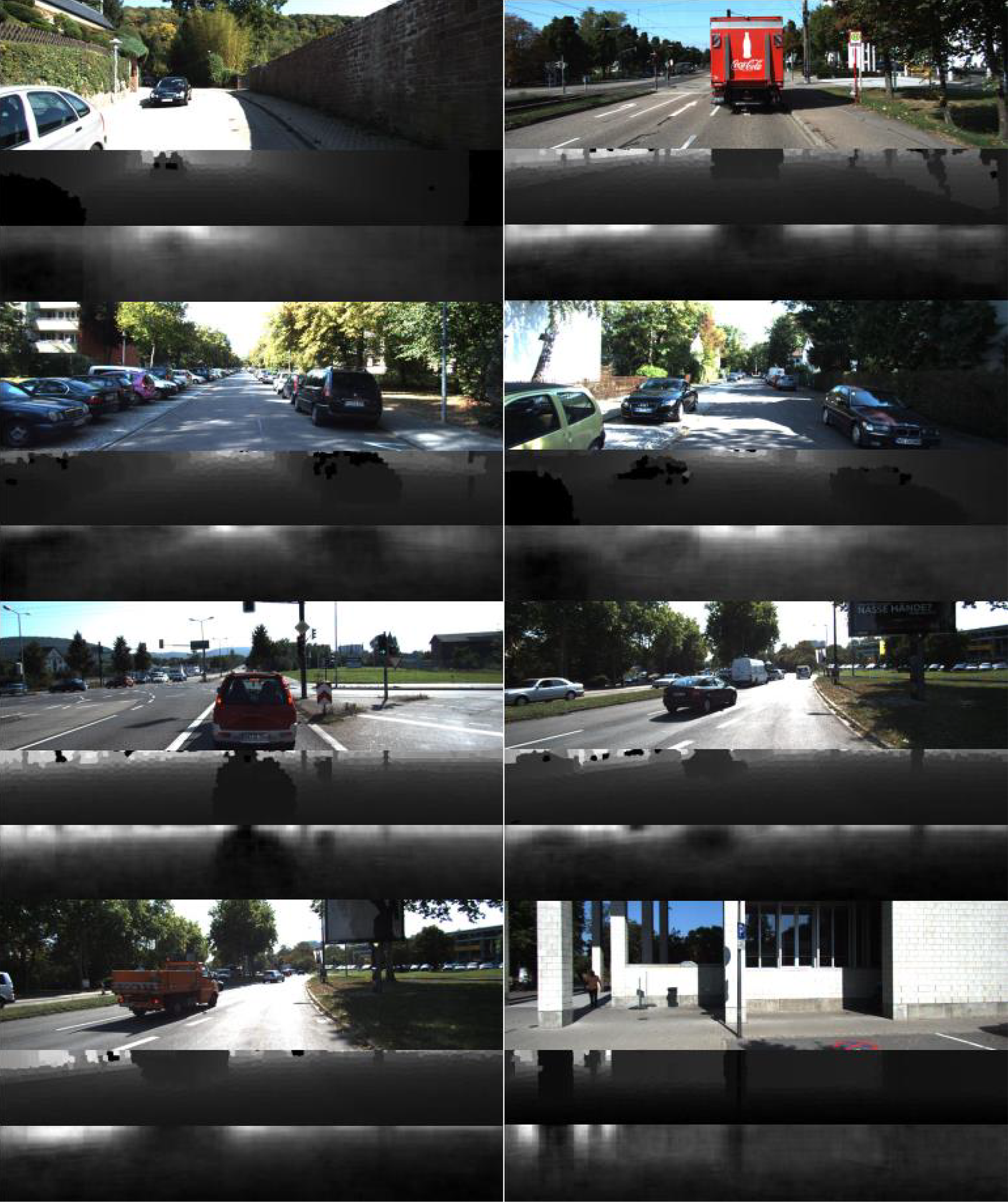
Example predictions from our algorithm. Every three rows of the figure constitute a group. For each input image, we show input (top row of each group), ground truth (middle row of each group), and output (bottom of each group). The values of the depth are normalized to [0–255].

As shown in Figure 5, the proposed method accurately predicts the depth of road scene images. It is also good for deep prediction in some details, such as small target objects in road scenes. Furthermore, the method can fill the holes existing in the real depth map of the road scene and obtain continuous depth information.

In Table 5, we compare our model with several popular methods. Besides, we set our method as a baseline and change our model to “single image input with skip connection” and “image sequence input without skip connection” as two comparative experiments. All the methods in the table used the same evaluation indicators, namely six indicators of $δ < 1.25$ , $δ < {1.25}^{2}$ , $δ < {1.25}^{3}$ , Rel, Linear RMSE, and Log RMSE. The higher the value of the first three indicators, the higher the accuracy.

Table 5.

Comparison on the KITTI data set.

	Threshold $δ < 1.25$	Threshold $δ < {1.25}^{2}$	Threshold $δ < {1.25}^{3}$	Rel	Linear RMSE	Log RMSE
Mean	0.556	0.752	0.870	0.412	9.635	0.444
Saxena et al. (Make3D)⁷	0.601	0.820	0.926	0.280	8.734	0.361
Eigen et al. (coarse)¹⁶	0.679	0.897	0.967	0.194	7.216	0.273
Eigen et al. (coarse + fine)¹⁶	0.692	0.899	0.967	0.190	7.156	0.270
Liu et al. (pre-train)³⁸	0.613	0.858	0.949	0.236	7.421	0.101
Liu et al. (fine-train)³⁸	0.656	0.881	0.958	0.217	7.046	0.096
Cao et al.³⁹	0.703	0.976	0.987	0.214	6.156	0.082
Mancini et al. (single img)⁴⁰	0.311	0.572	0.764	—	7.542	0.574
Mancini et al. (opt + img)⁴⁰	0.421	0.679	0.813	—	6.863	0.504
Xu et al.²¹	0.698	0.923	0.981	0.169	4.710	0.673
Wang et al. (DDVO)³²	0.808	0.946	0.983	0.147	5.183	1.014
Our (single input)	0.878	0.950	0.970	0.135	4.620	0.490
Our (no skip connection)	0.820	0.931	0.969	0.150	5.500	0.482
Our	0.892	0.970	0.988	0.119	3.462	0.162

Rel: Abs relative difference; Linear RMSE: linear root mean squared error; Log RMSE: log root mean squared error; 3-D: three dimensional; DDVO: differentiable direct visual odometry. Best performance is indicated with bold.

When compared to other methods, it can be observed that our method achieved the best evaluation results, when the thresholds $δ < 1.25$ and $δ < {1.25}^{3}$ . In particular, when $δ < 1.25$ , the accuracy of our method is nearly 0.2 higher than the second-place result. When the threshold is $δ < {1.25}^{2}$ , the second-highest accuracy is achieved with a score of 0.970, which is close to the accuracy of the first. These three δ threshold indicators indicate that the difference between our predicted value and the real value is the smallest in all comparison methods. Our method achieves the best evaluation results with an evaluation value of 0.119, which is nearly 0.1 lower than the second-place method in Rel. In Linear RMSE, our method achieved the first evaluation effect, and its evaluation value is far lower than in the second place. These two indicators show that the continuity of our predicted depth map has also achieved good results.

When compared to different versions of our methods, Table 5 shows that the results of the model with consecutive frames and skip connection is better than the incomplete models. The model of image sequence input without skip connection achieves better performance than the model of single image input with skip connection in $δ < 1.25$ , $δ < {1.25}^{2}$ , $δ < {1.25}^{3}$ , and Linear RMSE. The comparative experiment shows that the accuracy of the result is much worse when “skip” is removed from the network, and the accuracy of using only a single picture as input is not good enough. By comparison, we find that the combination of image sequence input and skip connection can get good results. We think that the consecutive frames can take more information, such as optical flow and consistency between consecutive frames, into the framework. Unlike the methods using stereo images, we take two neighboring images in a monocular video sequence as input. The proposed method does not need to estimate motion between images, which has fewer parameters and can achieve more integrated end-to-end training.

Of course, there are some methods that have achieved good results, such as Fu et al.³³ and Li et al.²² By comparison, we find that our method is not as good as the above two methods. We think the reasons may be as follows. First, the method proposed in this article is our earliest experiment. Second, we did not introduce additional information, nor did we perform detailed feature extraction on the ground truth values.

Conclusion

We proposed a method for depth estimation of road scene video images based on the FCN network and skip connection. The method takes continuous image frames and corresponding real depth information as input, and skip connection and multi-layer deconvolution networks are used to preserve more information and output pixel-level results. With the integration framework that combines skip connection, FCN network and the consistency between consecutive frames of the input sequence, high-resolution depth maps are obtained with lightweight network training and fewer computations. The proposed method models depth estimation as a regression problem and trains the proposed network using a scale invariance optimization based on L2 loss function, which measures the relationships between points in the consecutive frames. The whole neural network is constructed by image convolutional coding and deconvolution decoding, which overcomes the problem that the traditional method based on CNN cannot output a full-scale depth estimation map. Further, the method adopts the convolutional coding part and the deconvolution decoding part of the convolutional layer hopping link to realize a more flexible network structure, and it provides more reference information for the subsequent decoding part, compared with simple upsampling. The method can achieve better depth estimation results. In the experimental part of this article, we demonstrated that our approach performs surprisingly well.

In future work, we think that unsupervised learning or half-supervised learning is very important for depth estimation due to the lack of annotation data. Compared with supervised approaches, unsupervised approaches or half-supervised approaches could predict depth through minimizing the image reconstruction error without ground truth of input images during train. The key areas of our future work include unsupervised learning methods and multi-sensor fusion. The spacing-increasing discretization³³ strategy and deep attention-based classification²² strategy give us a lot of inspiration. We believe that the methods are very worthy of reference for our future work.

Footnotes

Acknowledgement

The authors would like to thank the reviewers for spending their valuable time on this article.

Declaration of conflicting interests

The author(s) declared no potential conflicts of interest with respect to the research, authorship, and/or publication of this article.

Funding

The author(s) disclosed receipt of the following financial support for the research, authorship, and/or publication of this article: This work was supported by the National Natural Science Foundation of China (61773245, 61603068, 61806113), Natural Science Foundation of Shandong Province (ZR2018ZC0436, ZR2018PF011, ZR2018BF020), Key Research and Development Program of Shandong Province (2018GGX101053), Scientific Research Foundation of Shandong University of Science and Technology for Recruited Talents (2017RCJJ061, 2017RCJJ062, 2017RCJJ063), and Taishan Scholarship Construction Engineering.

ORCID iDs

Zhiguo Zhang

Chunyang Sheng

References

Strecha

Fransens

Van Gool

Combined depth and outlier estimation in multi-view stereo. In: 2006 IEEE Computer Society conference on computer vision and pattern recognition (CVPR’06), vol. 2, New York, NY, USA, 17–22 June 2006, pp. 2394–2401. IEEE.

Liu

Dobaie

, et al. Autonomous road detection and modeling for UGVs using vision-laser data fusion. Neurocomputing 2018; 275: 2752–2761.

Sun

Zheng

Shum

. Stereo matching using belief propagation. IEEE T Pattern Anal Mach Intell 2003; 25(7): 787–800.

Gupta

Efros

Hebert

. Blocks world revisited: image understanding using qualitative geometry and mechanics. In: European conference on computer vision, 5 September 2010, pp. 482–496. Cham: Springer.

Zhang

Tsai

Cryer

, et al. Shape-from-shading: a survey. IEEE T Pattern Anal Mach Intell 1999; 21(8): 690–706.

Snavely

Seitz

Szeliski

. Photo tourism: exploring photo collections in 3D. In: ACM transactions on graphics (TOG), vol. 25, 1 July 2006, pp. 835–846. New York: ACM.

Saxena

Sun

. Make3D: learning 3D scene structure from a single still image. IEEE T Pattern Anal Mach Intell 2009; 31(5): 824–840.

Shen

Dai

, et al. Depth and surface normal estimation from monocular images using regression on deep features and hierarchical CRFs. In: Proceedings of the IEEE conference on computer vision and pattern recognition, Boston, MA, USA, 7–12 June 2015, pp. 1119–1127.

Liu

Salzmann

Discrete-continuous depth estimation from a single image. In: Proceedings of the IEEE conference on computer vision and pattern recognition, Columbus, OH, USA, 23–28 June 2014, pp. 716–723.

10.

Wang

Shen

Lin

, et al. Towards unified depth and semantic prediction from a single image. In: Proceedings of the IEEE conference on computer vision and pattern recognition, Boston, MA, USA, 7–12 June 2015, pp. 2800–2809.

11.

Karsch

Liu

Kang

. Depth extraction from video using non-parametric sampling-supplemental material. In: Proceedings of the 12th European conference on computer vision, vol. part V, pp. 775–788. Berlin: Springer, 2012.

12.

Karsch

Liu

Kang

. Depth transfer: depth extraction from video using non-parametric sampling. IEEE T Pattern Anal Mach Intell 2014; 36(11): 2144–2158.

13.

Konrad

Wang

Ishwar

. 2D-to-3D image conversion by learning depth from examples. In: 2012 IEEE Computer Society conference on computer vision and pattern recognition workshops (CVPRW), 16–21 June 2012, Providence, RI, USA, pp. 16–22. IEEE.

14.

Krizhevsky

Sutskever

Hinton

. ImageNet classification with deep convolutional neural networks. In: Proceedings of the 25th international conference on neural information processing systems, vol. 1, Lake Tahoe, NV, USA, pp. 1097–1105. Red Hook, NY: Curran, pp. 1097–1105.

15.

Simonyan

Zisserman

. Very deep convolutional networks for large-scale image recognition. arXiv preprint arXiv:14091556, 2014.

16.

Eigen

Puhrsch

Fergus

. Depth map prediction from a single image using a multi-scale deep network. In: Advances in neural information processing systems, Montreal, Canada, 8–13 December 2014, pp. 2366–2374.

17.

Eigen

Fergus

Predicting depth, surface normal and semantic labels with a common multi-scale convolutional architecture. In: Proceedings of the IEEE international conference on computer vision, Santiago, Chile, 7–13 December 2015, pp. 2650–2658.

18.

Roy

Todorovic

Monocular depth estimation using neural regression forest. In: Proceedings of the IEEE conference on computer vision and pattern recognition, Las Vegas, NV, USA, 27–30 June 2016, pp. 5506–5514.

19.

Liu

Shen

Lin

. Deep convolutional neural fields for depth estimation from a single image. In: Proceedings of the IEEE conference on computer vision and pattern recognition, Boston, MA, USA, 7–12 June 2015, pp. 5162–5170.

20.

Kim

Park

Sohn

, et al. Unified depth prediction and intrinsic image decomposition from a single image via joint convolutional neural fields. In: European conference on computer vision, Boston, MA, USA, 7–12 June 2015, pp. 143–159. Cham: Springer.

21.

Ricci

Ouyang

, et al. Multi-scale continuous CRFs as sequential deep networks for monocular depth estimation. In: Proceedings of CVPR, vol. 1, Honolulu, HI, USA, 4 July 2017.

22.

Xian

Shen

, et al. Deep attention-based classification network for robust depth prediction. In: Asian conference on computer vision, Perth, Australia, 2–6 December 2018, pp. 663–678. Cham: Springer.

23.

Dai

, et al. R-FCN: object detection via region-based fully convolutional networks. In: Advances in neural information processing systems, Barcelona, Spain, 20–21 May 2016, pp. 379–387.

24.

Lin

Dollár

Girshick

, et al. Feature pyramid networks for object detection. In: Proceedings of the IEEE conference on computer vision and pattern recognition, Honolulu, HI, USA, 21–26 July 2017, pp. 2117–2125.

25.

Ronneberger

Fischer

Brox

. U-Net: convolutional networks for biomedical image segmentation. In: International conference on medical image computing and computer-assisted intervention, Shenzhen, China, 13–17 October 2019, pp. 234–241. Cham: Springer.

26.

Chen

Papandreou

Kokkinos

, et al. DeepLab: semantic image segmentation with deep convolutional nets, atrous convolution, and fully connected CRFs. IEEE T Pattern Anal Mach Intell 2017; 40(4): 834–848.

27.

Badrinarayanan

Kendall

Cipolla

SegNet: a deep convolutional encoder-decoder architecture for image segmentation. IEEE T Pattern Anal Mach Intell 2017; 39(12): 2481–2495.

28.

Qiu

Zhuang

Yan

, et al. RGB-DI images and full convolution neural network-based outdoor scene understanding for mobile robots. IEEE T Instrum Meas 2019; 68: 27–37.

29.

Godard

Mac Aodha

Brostow

. Unsupervised monocular depth estimation with left-right consistency. In: Proceedings of the IEEE conference on computer vision and pattern recognition, Honolulu, HI, USA, 21–26 July 2017, pp. 270–279.

30.

Zhou

Brown

Snavely

, et al. Unsupervised learning of depth and ego-motion from video. In: Proceedings of the IEEE conference on computer vision and pattern recognition, Honolulu, HI, USA, 21–26 July 2017, pp. 1851–1858.

31.

Godard

Mac Aodha

Firman

, et al. Digging into self-supervised monocular depth estimation. In: Proceedings of the IEEE international conference on computer vision, Seoul, South Korea, 27 October–2 November 2019, pp. 3828–3838.

32.

Wang

Miguel Buenaposada

Zhu

, et al. Learning depth from monocular videos using direct methods. In: Proceedings of the IEEE conference on computer vision and pattern recognition, Salt Lake City, UT, USA, 18–23 June 2018, pp. 2022–2030.

33.

Gong

Wang

, et al. Deep ordinal regression network for monocular depth estimation. In: Proceedings of the IEEE conference on computer vision and pattern recognition, Salt Lake City, UT, USA, 18–23 June 2018, pp. 2002–2011.

34.

Long

Shelhamer

Darrell

Fully convolutional networks for semantic segmentation. In: Proceedings of the IEEE conference on computer vision and pattern recognition, Boston, MA, USA, 7–12 June 2015, pp. 3431–3440.

35.

Kuznietsov

Stuckler

Leibe

Semi-supervised deep learning for monocular depth map prediction. In: Proceedings of the IEEE conference on computer vision and pattern recognition, Honolulu, HI, USA, 21–26 July 2017, pp. 6647–6655.

36.

Vijayanarasimhan

Ricco

Schmid

, et al. SfM-Net: learning of structure and motion from video. arXiv preprint arXiv:170407804, 2017.

37.

Geiger

. Are we ready for autonomous driving? The KITTI vision benchmark suite. In: Computer vision and pattern recognition, Providence, RI, USA, 16–21 June 2012, pp. 3354–3361.

38.

Liu

Shen

Lin

, et al. Learning depth from single monocular images using deep convolutional neural fields. IEEE Trans Pattern Anal Mach Intell 2016; 38(10): 2024–2039.

39.

Cao

Shen

. Estimating depth from monocular images as classification using deep fully convolutional residual networks. IEEE Trans Circuits Syst Video Technol 2018; 28: 3174–3182.

40.

Mancini

Costante

Valigi

, et al. Fast robust monocular depth estimation for obstacle detection with fully convolutional networks. In: IEEE/RSJ international conference on intelligent robots and systems (IROS), Daejeon, South Korea, 9–14 October 2016, pp. 4296–4303. IEEE.

Depth estimation for a road scene using a monocular image sequence based on fully convolutional neural network

Abstract

Keywords

Introduction

Network architecture

Architecture

Loss function

Experiments

Experimental setup

KITTI data set

Data augmentation

Evaluation metrics

Experimental parameters

Experimental results

Conclusion

Footnotes

Acknowledgement

Declaration of conflicting interests

Funding

ORCID iDs

References