
Abstract
Devices that measure our physical, medical and mental condition have entered our daily life recently. Such devices measure our status in a continuous manner and can be useful in predicting future medical events or can guide us towards a healthier life. It is therefore important to establish that such devices record our behaviour in a reliable manner and measure what we believe they measure. In this article, we propose to measure the reliability and validity of a newly developed measuring device in time using a longitudinal model for sequential kappa statistics. We propose a Bayesian estimation procedure. The method is illustrated by a validation study of a new accelerometer in cardiopulmonary rehabilitation patients.
Introduction
The future in many scientific domains lies in devices recording continuously and in real-time biological, physical, behavioural or environmental information. These devices offer the possibility to study individuals in their natural environment and can provide real-time personalized feedback. For example, physical activity can be assessed in real-time using activity trackers. The devices produce intensive longitudinal data, characterized by a large amount of observations (e.g., thousands), often very close in time (e.g., every second) and collected on every individual of a sample over a short time period (Bolger and Laurenceau (2013)).
Despite the diversity of uses and purposes, it is imperative for all these devices to be reliable (provide consistent measurements) and valid (measure what it is meant to be measured). Lack of reliability and validity can lead to incorrect conclusions from scientific studies and unreproducible research (Munafo et al.(2017)Munafo, Nosek, Bishop, Button, Chambers, Percie du Sert, Simonsohn, Wegenmakers, Ware, and Ioannidis). The picture is equally bleak for every day users, who will be unable to assess changes in any biological, physical, behavioural or environmental information provided by the measurement instruments. Reliability refers to the ability in differentiating between items in a population. This is an essential property of a measurement scale, especially when assessing the correlation with other measures because of the well-known attenuation effect. On top of good reliability, good agreement is also sometimes imperative, as in clinical decision-making where the decision depends on the score provided by observers/devices. Agreement is also an important concept when studying criterion validity, where the measurement instrument is calibrated against an established method. The established method is often regarded as a ‘gold standard’ measuring the ‘true value’ of the quantity to be determined. However, it is frequent that also the reference method is subject to measurement error. In that case, the comparability of the new and the reference methods is assessed by the degree of agreement between them.
It is important to assess reliability and agreement in realistic settings on the target user groups on top of controlled laboratory conditions. Subjects may behave differently in real life as compared to laboratory settings, impacting the reliability/agreement levels. This was the case in the CAM study (Annegarn et al.(2011)Annegarn, Spruit, Uszko-Lencer, Vanbelle, Savelberg, Schols, Wouters, and Meijer), motivating this article. The CAM study was designed to validate a new accelerometry sensor, the Movement in a bOX (MOX, initially named CAM) in real conditions. The MOX can categorize body activity as non-weight bearing (e.g., lying or sitting), weight bearing (e.g., standing) or dynamic (e.g., walking). This device was developed to be an objective alternative to questionnaires when measuring physical activity during the revalidation of patients with chronic organ failure. During one hour of unconstrained activity, 10 patients with chronic organ failure were videotaped in a revalidation centre while their body activity was continuously recorded with the MOX, worn simultaneously on the leg and on the trunk for comparative purposes. The aims were (a) to determine the validity of the new accelerometry sensor through the agreement level between MOX recordings and human observations of body activity on the videotape considered as the reference method; (b) to assess temporal stability of the validity levels (e.g., validity levels can decrease because of device shifts); and (c) to determine the influence of the body location where the device is held on the validity levels.
When two observers (or devices) classify items (subjects/objects) on nominal scales, Cohen's kappa coefficient (Cohen (1960)) is an appropriate agreement measure and the intraclass kappa coefficient (Kraemer (1979)) an appropriate reliability measure. Kappa coefficients have the particularity to take the marginal probability distribution of the observers into account, which is often a desirable property. These coefficients were extended over the years to account for predictors under various study designs including longitudinal settings. However, intensive longitudinal data, as produced by accelerometers, differ from longitudinal data in many respects (Walls and Schafer (2006)). First, they often show complex trajectories, including cyclic patterns or chaotic elements over time that can wildly vary between subjects. If poorly modelled, biased estimates of agreement and reliability levels can be obtained. Second, observations close in time often exhibit serial correlation. Ignoring this correlation will lead to incorrect conclusions regarding the reliability and agreement levels. In particular, reliability and agreement are likely to be overestimated, resulting in daily-life use of measurement instruments less reliable and valid than expected. Third, studies with intensive longitudinal data often involve a small number of subjects (10 in the CAM study) due to the high costs of studies involving these cutting edge technologies and many observations per subject (3 600 in the CAM study) due to the recording speed and storage properties of the electronic devices. The combination of these two latter facts leads to computational problems and instability in the parameter estimates when using the existing unit-specific models (Gajewski et al.(2007)Gajewski, Hart, Bergquist-Beringer, and Dunton; Hsiao et al.(2011)Hsiao, Chen, and Kao; Vanbelle et al.(2012)Vanbelle, Mutsvari, Declerck, and Lesaffre; Tsai (2012); Vanbelle and Lesaffre (2015)), such as multilevel models, and population-based approaches (Klar et al.(2000)Klar, Lipsitz, and Ibrahim; Williamson et al.(2000)Williamson, Lipsitz, and Manatunga; Gonin et al.(2000)Gonin, Lipsitz, Fitzmaurice, and Molenberghs), like generalized estimating equations. This is especially true when the number of measurement occasions surpasses the number of participants (Little et al.(2017)Little, Wang, and Gorrall), as in the CAM study and therefore prevents the use of these methods in the current context.
One simple solution is to summarize the information over time intervals and therefore reduce the number of repeated measurements. For example, define one minute intervals and determine the time spent under each body activity within these intervals. Then, the aforementioned methods on the reduced data could eventually be applied. This practice, encountered in behavioural sciences (Rapp et al.(2011)Rapp, Carroll, Stangeland, Swanson, and Higgins; Liu et al.(2016)Liu, Zhou, Palumbo, and Wang), should be avoided in the context of agreement studies. The most obvious reason is that summary measures can perfectly agree (e.g., two methods recorded 25 seconds duration in non-weight bearing posture) when perfect disagreement is observed in the raw data (e.g., the first method recorded the 25 first seconds and the second method the 25 last seconds of the interval as non-weight bearing posture). Ignoring these disagreements can lead to incorrect conclusions when using the measurement instrument to study process dynamics.
This let us to develop a new partial-Bayesian methodology, on the ground of Vanbelle and Lesaffre (2015), permitting the direct evaluation of the impact of predictors on the agreement levels obtained on intensive longitudinal data. The new method extends the method of Vanbelle and Lesaffre (2015) in two ways. First, it permits to summarize the information over time intervals without loss of information over disagreement in the raw data. Second, the method permits to account for possible correlation both within and between time intervals. We describe the motivating data in Section 2. After extending the definition of the kappa coefficient to intensive longitudinal data in Section 3, we introduce the methodology to model agreement obtained on intensive longitudinal data in Section 4. The results of the CAM study are presented in Section 5. A simulation study is conducted in Section 6. Finally, the methodology is discussed in Section 7.
Motivating data: The CAM study
Patients with chronic organ failure are generally characterized by an inactive lifestyle to avoid the unpleasant sensation of dyspnea. Decreased weight-bearing activities and postures in daily life (e.g., walking and standing) are important triggers in the development and/or progression of lower-limb muscle atrophy, muscle weakness and exercise intolerance in patients with chronic organ failure (Annegarn et al.(2011)Annegarn, Spruit, Uszko-Lencer, Vanbelle, Savelberg, Schols, Wouters, and Meijer). To implement daily physical activity as an outcome measure of cardiopulmonary rehabilitation, Annegarn et al.(2011)Annegarn, Spruit, Uszko-Lencer, Vanbelle, Savelberg, Schols, Wouters, and Meijer wanted to validate in real settings a new accelerometry sensor, the MOX, developed within Maastricht University by the service point Activity Monitoring.
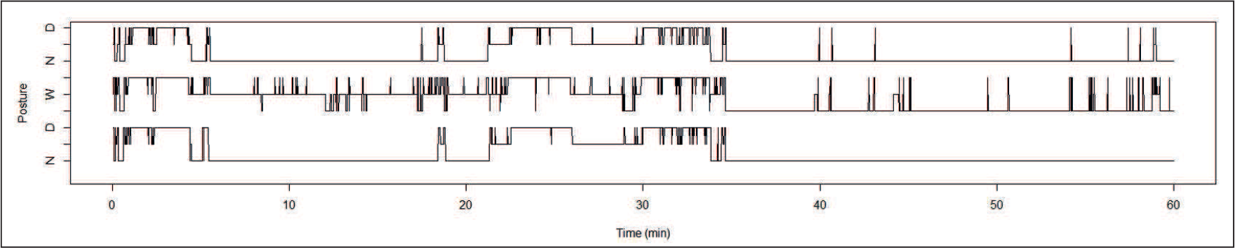
To that end, 10 patients were recruited during their rehabilitation programme at CIRO+, a centre of expertise for chronic organ failure in Horn (The Netherlands). The patients were asked to wear the MOX at two different body places simultaneously, namely on the leg (frontal part of the thigh) and on the trunk (lower back) for one hour during their daily activities. These patients were also videotaped everywhere when wearing the MOX, except in the toilets. The subject's activity (non-weight bearing posture, weight bearing posture or dynamic activity) was also determined every second on the video by a researcher, blinded to the values obtained with the MOX. The records of one subject are displayed in Figure 1.
CAM study. Activity (N = non-weight bearing posture, W = weight-bearing posture and D = dynamic activity) recorded with the video (bottom), the MOX worn on the trunk (middle) and on the leg (top) for one subject
CAM study. Activity (N = non-weight bearing posture, W = weight-bearing posture and D = dynamic activity) recorded with the video (bottom), the MOX worn on the trunk (middle) and on the leg (top) for one subject
The aims were (a) to determine the validity of the new sensor in real settings through the agreement level between MOX recordings and human observations of body activity on the videotape considered as the reference method; (b) to assess temporal stability of the validity levels (e.g., validity levels can decrease because of device shifts); and (c) to determine the influence of the body location where the device is held on the validity levels.
In this article, we focus on the distinction between non-weight bearing postures (NWBP) on one hand and weight-bearing postures and dynamic activities on another hand, because these two latter positions have both to be encouraged during the rehabilitation process.
Introduction
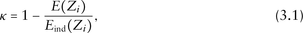
Kappa coefficients are defined in terms of population parameters similarly to Vanbelle (2016). Consider two fixed observers classifying a sample of items (subjects or objects) from population
Cohen's kappa coefficient is defined as
where
The definition of the kappa coefficients is based on independent
Suppose that two observers (or devices) classify on a binary scale a sequence of
Let
Suppose that the observation period is divided into small time intervals. The intervals can be of unequal lengths but assume, for notational convenience that the sequence of
The first condition holds by construction of the time intervals. The second condition is not necessarily met. However, taking the average probability over a time interval corresponds to temporal aggregation, a smoothing technique used in time series analysis (see, e.g., Silvestrini and Veredas (2008)). In particular, flow aggregation consists in taking the sum of variables over time intervals as aggregated variable. Finally, the third condition does not hold. Observations close in time are very likely to be correlated. To relax this third assumption, the binomial distribution is replaced by a beta-binomial distribution. The additional overdispersion parameter in the beta-binomial distribution
The random variable
Then, the agreement coefficient in the

Equation 3.2 also defines
Statistical model
The aim is to relate the agreement coefficient
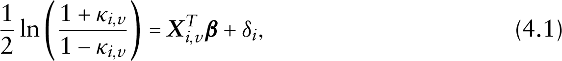
where
In the same way, the probability to be classified in category 1 will be related to predictors through the random effects model

where
Suppose now that we have followed up subjects intensively in a short period of time providing continuous measurements from different observers or measurement devices. From the records we establish whether or not they agree. Namely, suppose that we obtained

is considered where the index
The within-interval correlation is captured through the overdispersion parameter in the beta-binomial distributions. By considering beta-binomial distributions, the correlation between observations belonging to the same time interval is an intraclass correlation coefficient and is therefore restricted to be positive. Values close to 0 indicate heterogeneity in the observations within time intervals while values close to 1 indicate homogeneity. This could help in determining the adequacy of the time intervals length. Namely, a relatively high intraclass correlation means that observations within a time interval are homogeneous, supporting the temporal aggregation assumption.
Between-interval correlations
Between-interval correlations of derived measures from the intensive longitudinal data may give extra insight in the stability of these measures over time. One popular choice in this context, is again the intraclass correlation. However, in the presence of a binary outcome and covariates the intraclass correlation is less straightforward to compute. Goldstein et al. (2002) Goldstein, Browne, and Rasbash developed three approaches to estimate the intraclass correlation for binomial random variables. To be used in our context, we extended their simulation approach to beta-binomial random variables in the Bayesian framework. We refer to Appendix B for the calculation of the intraclass correlation for kappa coefficients (Eqn. 4.1) and marginal probabilities (Eqn. 4.2).
Bayesian estimation
Maximum likelihood estimation of the model parameters from the above pseudo-likelihood proves to be quite difficult. We therefore adopted the partial-Bayesian approach suggested in Vanbelle and Lesaffre (2015) using Markov chain Monte Carlo (MCMC). The frequentist coverage of Bayesian confidence intervals has been shown to be excellent in Vanbelle and Lesaffre (2015) and is often quite good, see, for example, Lesaffre and Lawson (2012). It is also often better than using the Delta method, which needs asymptotic arguments and often leads to too narrow confidence intervals (Efron (1992)), especially if non-linear functions are involved, as it is the case in Eqn. 4.1. Because of the limited number of subjects, parsimony was needed in the modelling approach. The two overdispersion parameters,
We used vague priors which express the lack of prior information on the parameters. For the regression coefficients
CAM study
The activity (non-weight bearing, weight bearing, dynamic) of 10 patients with chronic organ failure was recorded every second during 1 hour by the new accelerometry sensor, the MOX, worn simultaneously on the leg and on the trunk. The patients were also videotaped when wearing the device and the activity was then assessed every second by a researcher. The video is considered as the reference method. The agreement level between the new device and the video is determined. Agreement levels obtained for the trunk and the leg are then compared.
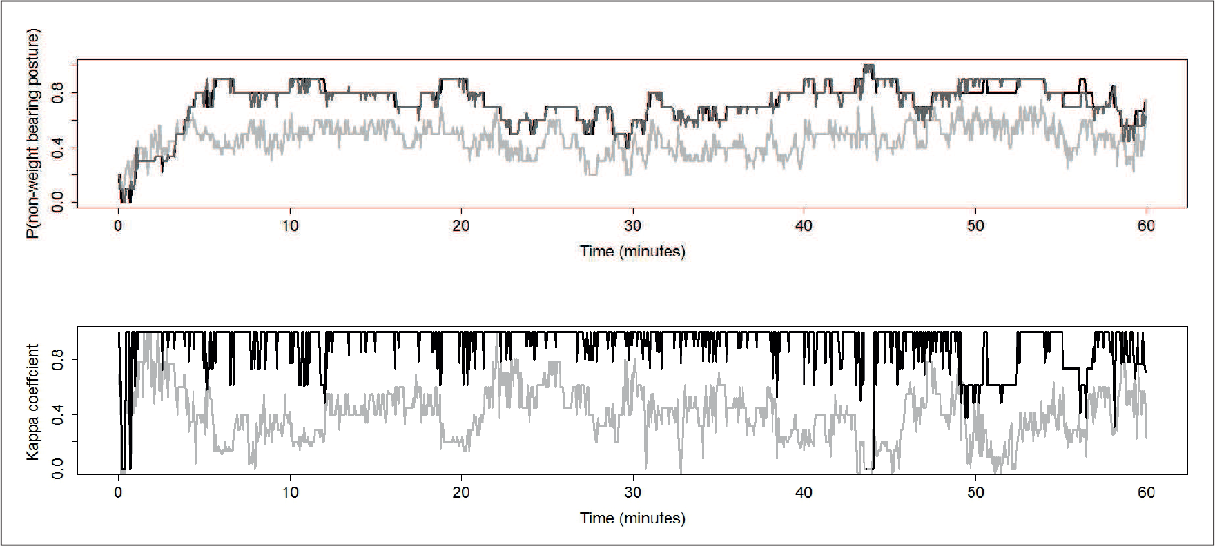
The probability to be in a non-weight bearing posture (NWBP) and the agreement level between the MOX and the video assessments are displayed in Figure 2 over the one hour observation period. These quantities were determined over 2 seconds intervals to be graphically displayed. The probability to be in a NWBP seems to vary over time and differs markedly between MOX (trunk) on one hand and MOX (Leg) and video on the other hand. This will obviously lead to different agreement levels for the MOX(trunk) and the MOX(leg). A burnin period of 5 minutes after the device placement was discarded from the data when applying the modelling approach as all patients were standing to have the MOX device installed.
CAM study. Top: Evolution of the probability of being in a NWBP over the one hour observation period with the MOX worn on the trunk (light grey), on the leg (dark grey) and by the observer on the video (black). Bottom: Agreement (kappa) between the video and the MOX worn on the leg (black) and on the trunk (light grey)
CAM study. Top: Evolution of the probability of being in a NWBP over the one hour observation period with the MOX worn on the trunk (light grey), on the leg (dark grey) and by the observer on the video (black). Bottom: Agreement (kappa) between the video and the MOX worn on the leg (black) and on the trunk (light grey)
No specific pattern in the shape of the evolution over time of the probability to be in a NWBP was expected or of direct interest since patients were studied in unconstrained real conditions at different moments of the day. The probability to be in NWBP is therefore modelled non-parametrically using low-rank thin plate splines (Wood (2003)). This leads to the following hierarchical probit regression model for the marginal probabilities
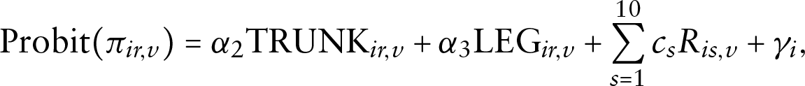
where TRUNK equals 1 if the device is the MOX worn on the trunk and equals 0 otherwise, LEG equals 1 if the device is the MOX worn on the leg and equals 0 otherwise. The coefficients
For the agreement, the interest is in the existence of any trend in the evolution of the agreement levels over time (i.e., stability of agreement) and in the comparison of the agreement level between the video and the MOX worn at two body places. This leads to the following model,

where TRUNK2 equals 1 if the agreement between the MOX(trunk) and the video is considered and 0 if the agreement between the MOX(leg) and the video is considered. The coefficients
For modelling purposes, we analysed the data twice, once with time intervals of 30 seconds and once with time intervals of 60 seconds. The data and R code are available as supplementary Web material. The posterior distribution of the marginal probability distribution and the agreement levels is summarized in Table 1 for 30 and 60 seconds intervals by using 10 equally spaced knots. The results with 10, 15 and 20 equally spaced knots were very similar (not shown).
Posterior distribution of the hierarchical probit regression model corresponding to the marginal probability distribution of the devices and the regression model for the agreement coefficient for 30 and 60 seconds intervals using 10 knots
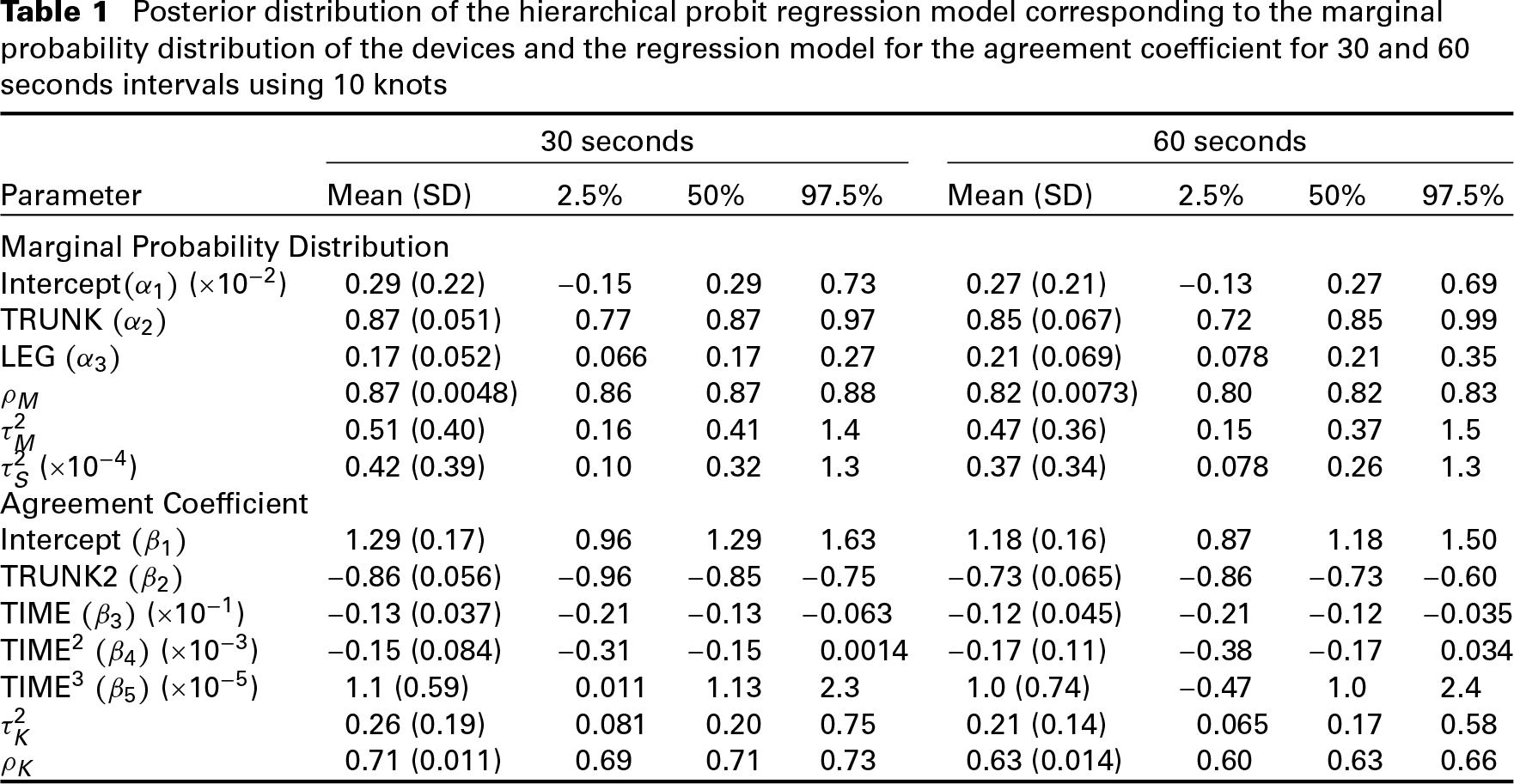
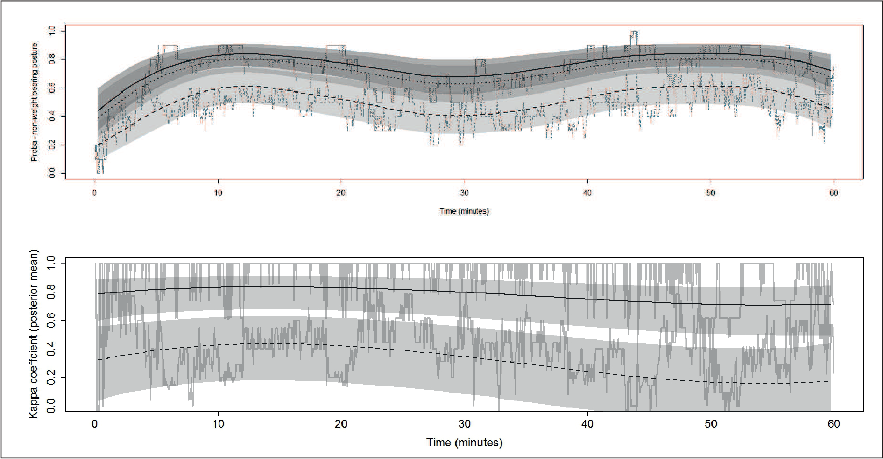
As seen in Table 1, the parameter estimates obtained with the 30 seconds model and the 60 seconds model are very similar. Given the random effects, the probability of recording NWBP differs between the video and the MOX worn at the two body places. The level of agreement between the MOX and the video records decreases with time and is higher for the MOX worn on the leg than on the trunk. The posterior distribution, obtained by averaging over the random effects, is depicted in Figure 3 for the marginal probability distribution and the agreement with pointwise 95% equal-tailed credibility intervals.
CAM study. Posterior distribution obtained by averaging over the random effects (pointwise 95% equal-tailed credibility interval) of the marginal probability distribution for the three devices (top) and of the agreement levels (bottom) when considering time intervals of 30 seconds. In the top panel, plain line is for video, dotted line for MOX(leg) and dashed line for MOX(Trunk). In the bottom panel, plain line is for MOX(leg) vs video and dashed line for MOX(Trunk) vs video
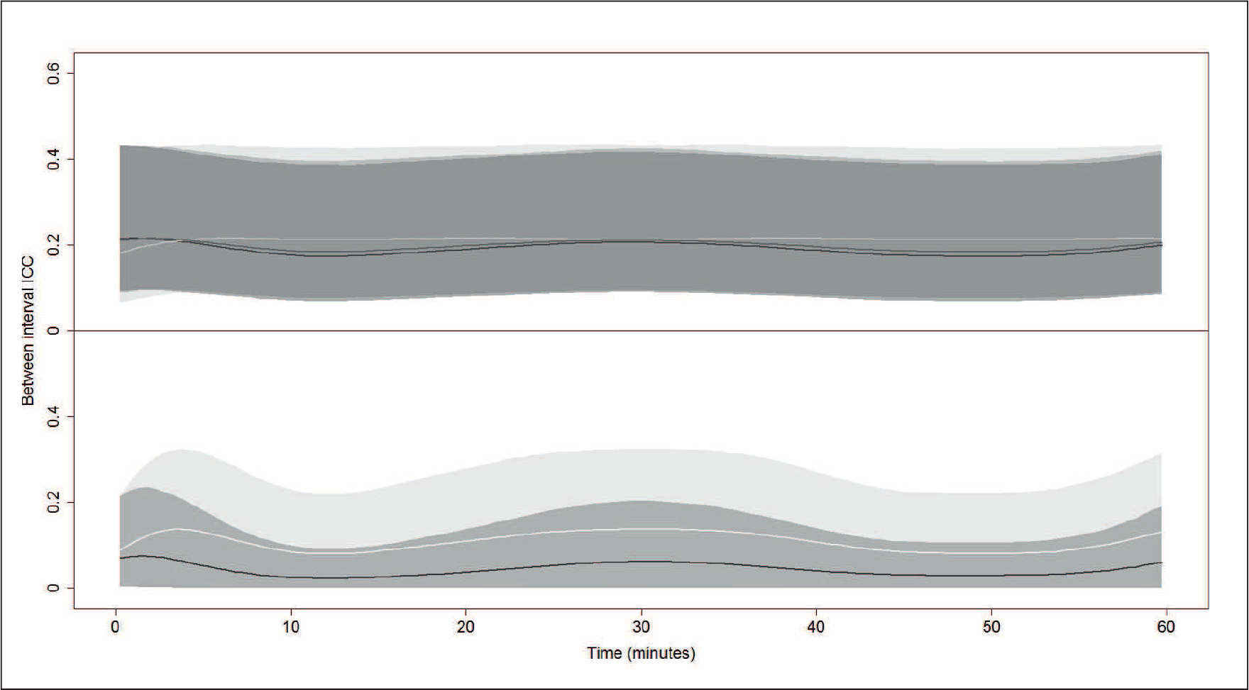
For 30 seconds intervals, the within-interval correlation is 0.87 [0.86,0.88] for the devices marginal probabilities and 0.71 [0.69,0.73] for the agreement coefficients. The between-interval correlation, as assessed by the intraclass correlation, is depicted over time in Figure 4 for each device. While the intraclass correlation is close and constant over time for the 3 device marginal probabilities, it is further apart for the two agreement coefficients.
CAM study. Posterior distribution obtained by averaging over the random effects (pointwise 95% equal-tailed credibility interval) of the between-interval intraclass correlation coefficient for devices marginal probabilities (top) and agreement coefficients (bottom) when considering time intervals of 30 seconds. In the top panel, black is for video, dark grey for MOX(leg) and light grey for MOX(Trunk). In the bottom panel, black is for MOX(leg) vs video and light grey for MOX(Trunk) vs video
Thus, we can conclude from our modelling exercise that the level of agreement with the video is better when the MOX was worn on the leg than on the trunk. This difference was however not observed in laboratory settings on healthy subjects (Annegarn et al.(2011)Annegarn, Spruit, Uszko-Lencer, Vanbelle, Savelberg, Schols, Wouters, and Meijer). Misclassification when the MOX was worn on the trunk mainly occurred because patients leaned forward while sitting to increase their ventilatory capacity. This forward sitting posture was classified as standing when the MOX was worn on the trunk, because gravitational accelerations in the anterior-posterior signal were in the range of the standing posture. A decrease of the agreement level between the MOX and the video was also observed over time. It is well known that kappa coefficients are influenced by the marginal probability distribution. The combination of a change of the probability of being in a NWBP over time with a small sample size could be partially responsible for variation in the agreement coefficient over time. However, this could be also an indication that the observation period was not long enough for the agreement level to reach a stable level or that the device shifted from the original position with time, decreasing the agreement levels.
Binary bivariate intensive longitudinal data were simulated using state-space models as follows. For every subject (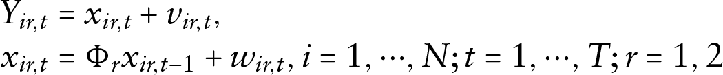
with

The corresponding correlation between
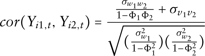
When the random variables

This permits to express
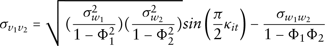
and therefore specify values for 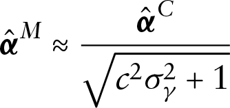
with 
Two scenarios were envisaged:
Scenario 1: Scenario 2:
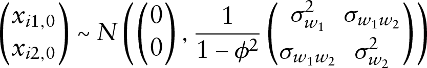
Starting values for the state equation were randomly chosen as
Before being analysed, the simulated bivariate AR(1) normal process was dichotomized at the value (0,0) to lead to a bivariate binary process. Data were summarized over intervals of 60 time points, leading to 15 time intervals. A total of 3 000 iterations with 2 000 burnin iterations were sufficient to attain convergence. The type I error rate, equal to the proportion of times the 95% equal-tailed credible interval does not cover the theoretical parameter values was determined for each simulation condition and reported in Table 2. For a simulation scheme with 1 000 simulated samples, the type I error rate is expected to be between 0.036 and 0.064.
Summary of the posterior distribution of the hierarchical agreement model over 1 000 simulated samples
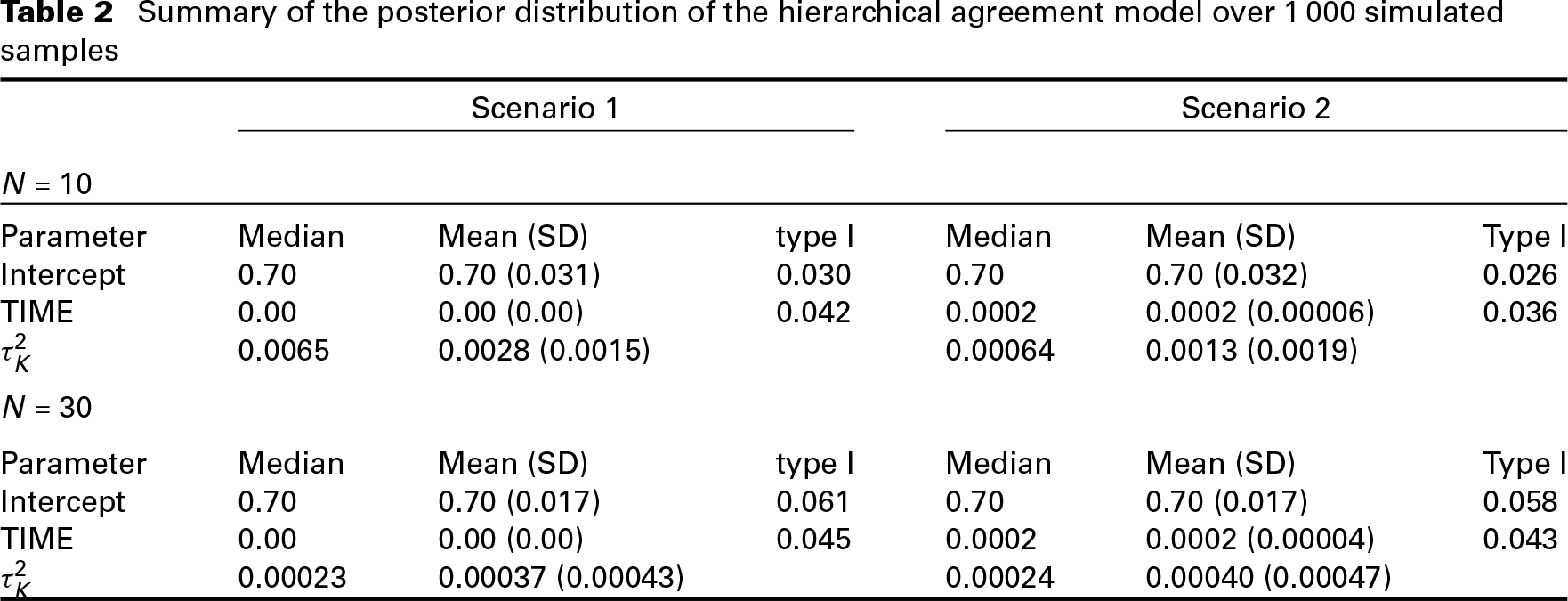
As seen in Table 2, the type I error is somewhat conservative for the intercept when the sample size is equal to 10. All simulation schemes led to a small random effect variance.
With the advent of measurement devices worn continuously by people to measure physical activities and medical conditions in daily life, we predict that intensive longitudinal data will become available abundantly in the future, especially in medical and psychological research. We argue that such devices will become increasingly important. For instance, some insurance companies are tracking your vitality using the measuring devices and offer rewards for those who have collected enough vitality points. In addition, such devices are currently incorporated in clinical trials. It is therefore important that such measuring devices reflect the true status of your activity over time.
In this article, we developed a methodology to study agreement in the presence of binary intensive longitudinal data. This method can be implemented in standard Bayesian software (e.g., Jags). We considered small time intervals and supposed that over the small time intervals, the agreement followed a beta-binomial distribution, accounting for the serial correlation within time intervals. We then proposed a partial-Bayesian methodology to directly evaluate the impact of categorical and continuous predictors, on Cohen's or the intraclass kappa coefficient. This method highlighted the effect of the position on the body where the MOX device was worn on the agreement level with the video records. The level of agreement with the video was better when the MOX was worn on the leg than on the trunk.
Several aspects of the proposed methodology need to be discussed. First, we believe that temporal aggregation makes sense. This is also confirmed by the large intra-interval correlation of 0.87 for the marginal probability distributions and 0.71 for the agreements. However, the length of the time intervals was arbitrarily fixed. The choice was suggested by the nature of the data (patients with chronic organ failure are not likely to change their position every second during rehabilitation). The length of the time intervals should be carefully chosen to consider all important pattern particularities in the data and to limit the effect of the assumption that the probability to be in a certain position is constant within time intervals (temporal aggregation). If the length of the time interval is too long, some pattern in the data can be hidden or some assumption (e.g., constant probability within an interval) might be breached. On the other hand, very short time intervals can lead to too much computational burden. Moreover, due to the small sample size, an additional assumption of constant overdispersion parameter for all time intervals and subjects had to be assumed. The use of constant overdispersion for all time intervals seems reasonable in this particular case since patients were observed under unconstrained conditions. There was therefore no reason to expect variation. For larger sample sizes, overdispersion parameters could further be modelled over time according to subject characteristics.
Second, choices were made to model the distribution of the data. First, the probability to classify items in category 1 and the probability to disagree were modelled using a beta-binomial distribution to account for possible correlation between the outcomes obtained at the different time points. The beta-binomial distribution was preferred over existing alternatives (see, e.g., Diniz et al.(2010)Diniz, Tutia, and Leite) because the distribution is available in Jags. Using alternative methods require to write explicitly the likelihood function. Second, the probit link function was used to model the probability to classify subjects in category 1. The logit link function is another option. The probit link was preferred because of the relationship between the kappa coefficient and the tetrachoric correlation coefficient under particular circumstances used in the simulation section (see Lord et al.(1968)Lord, Novick, and Birnbaum). Third, Fisher link function was introduced as a convenient way for modelling the kappa coefficient. This link function was chosen because it was developed to model the correlation coefficient (Fisher (1915)). Kappa coefficients present a similar behaviour. The complementary log-log function is an alternative. Fourth, splines were used to describe the evolution over time of the probability to be in non-weight bearing posture. This choice is motivated by the fact that we were not interested in the shape of the time evolution. When the evolution of the probability to classify items in category 1 is of interest, a parametric model should be preferred. Alternative splines approaches led to similar results in the present example.
Third, the method is based on a pseudo-likelihood rather than the full-likelihood. Vanbelle and Lesaffre (2015) have shown that in the context of multilevel modelling, using only part of the likelihood leads to somewhat higher standard errors for agreement coefficients when compared with a full-Bayesian approach, occurring principally for low agreement values, generally of little practical interest. Only limited simulation results were shown in the current context because of the difficulty to simulate bivariate binary intensive longitudinal data with a given trend in the agreement. Some conservatism was observed for the intercept when the sample size was equal to 10. Given the approximation between marginal and conditional parameters and given that the relationship between the tetrachoric coefficient and the kappa coefficient are only valid when the marginal probability distribution of the observers is exactly equal to 0.5, these simulation results are promising. More extended simulations are however needed.
In conclusion, we proposed a method to directly evaluate the effect of covariates on the level of agreement in the presence of binary continuous records. Future research to extend the method to continuous and ordinal scales is needed. An extension to spatio-temporal continuous records could be envisaged. \appendix
Footnotes
Supplementary material
Supplementary materials for this article, including data and R code, are available from
Acknowledgements
The authors thank the reviewers for their valuable comments. The authors are also grateful to Dr K. Meijer (Maastricht University) for providing the data and to Ayfer Ezgi Yilmaz, Department of Statistics, Hacettepe University, Ankara, Turkey.
Declaration of conflicting interests
The authors declared no potential conflicts of interest with respect to the research, authorship and/or publication of this article.
Funding
The authors disclosed receipt of the following financial support for the research, authorship and/or publication of this article: This research is part of project 451-13-002 funded by the Netherlands Organisation for Scientific Research.