Sage Journals: Discover world-class research

Abstract

The focus of this paper is on reducing vibrations and capturing energy from a three degrees-of-freedom (3DOF) dynamical system. The system consists of a damped spring-pendulum with an elliptical pivot path at a constant angular velocity and a connected rigid body experiencing external harmonic forces and moments. An independent electromagnetic energy harvesting system has been integrated into the structure, utilizing the motion of a magnet within a coil. The optimization efforts target both energy harvesting (EH) and vibration reduction capabilities. The second kind of Lagrange’s equations are used to formulate the governing kinematic equations, which are then solved asymptotically using the multiple-scales technique (MST), producing novel and precise results up to the third approximation. Various resonance cases are identified, with three examined concurrently. The time evolution of the solutions, as well as the modified phases and amplitudes, are analyzed through graphical representations, taking into account the influential parameters of the system. Graphical plots of phase portraits successfully depicted the system’s stable dynamics. The power output and current time profiles of the electromagnetic device are presented to demonstrate the impact of various parameters on system behavior. Analysis of stability and instability areas reveals that the system exhibits stable performance across a wide range of parameters. This model is gaining significance in contemporary applications, especially in control sensors used across various sectors such as industry, construction, automotive, transportation, and infrastructure.

Keywords

Nonlinear oscillations energy harvesting perturbation techniques resonance fixed points stability

Introduction

Over the past few decades, a great deal of study has been done on reducing damaging vibrations in a variety of architectural structures, including robotic limbs, high-rise buildings, bridges, spires, and turbines.¹ Vibration energy is an intriguing new energy source that is both sustainable and renewable. The process involves converting vibrational kinetic energy into unstable electrical power by scavenging, or the use of large amplitude vibrations for energy harvesting. Vibrations, mechanical strain, and stress in mechanical systems can all be effectively captured by this process. Furthermore, EH has shown to be a perfect option for supplying power to tiny gadgets such as wireless sensors.^2,3

The limitation of reliable power sources has spurred the growing adoption of mobile and cordless technologies into daily routines. Depending on bulky batteries that require frequent replacement for certain devices poses significant challenges. Hence, integrating EH as the primary power source for small-scale systems emerges as a practical solution. Leveraging sources such as sunlight, vibrations, and heat enables the swapping of temporary energy reservoirs with consistently charged energy storage components for a continuous power supply.^4–6 Energy extraction from these origins employs electromagnetic conversion, electrostatic, or piezoelectric methods. However, the oscillations produced usually function within lower frequency ranges, resulting in comparatively modest power outputs. As a result, the EH from these mechanisms typically falls within the micro to milliwatt range.^7–13

Electromagnetic energy harvesters harness the principles of Faraday’s induction law, which dictates that any alteration in the magnetic field surrounding a wire coil will induce an electromotive force within the coil. This phenomenon occurs when a magnet moves relative to the coil.¹⁴ Electrostatic transmutation, on the other hand, employs capacitors to convert mechanical energy into an electric field. By utilizing a variable capacitor, it functions as a current source capable of powering an electric circuit.¹⁵ Meanwhile, piezoelectric materials generate an electric field when subjected to pressure, leading to voltage generation when deformed under stress.¹⁶

In Ref. [17], the MST is employed to analyze an electromagnetic elastic-pendulum harvester model, focusing specifically on a two-to-one ratio of vibratory energy harvesters. In Ref. [18], the authors explore techniques for minimizing vibrations and capturing energy from a spring-pendulum system that moves along an elliptical trajectory. The pendulum’s structure is modified to integrate a separate electromagnetic harvesting system. In Ref. [19], the nonlinear movement of a connected damped pendulum to electromagnetic and piezoelectric devices is explored, employing approximate solutions and graphical representations to assess EH performance.

In Ref. [20], a novel strategy is introduced to enhance the efficiency of energy harvesting under low excitation conditions. This method involves incorporating a piezoelectric element attached to an inverted beam and pendulum system. Validation of this approach is achieved through an extensive finite element model, yielding valuable insights and simulations. Additionally,²¹ investigates the application of a pendulum-based harvester to tap into the energy generated by vibrations from high-speed train motion. Expanding on this theme, Ref. [22] taps into the behavior of the base of a double pendulum under excitation to generate electric energy on a small level. Notably, there exists a qualitative alignment between numerical and experimental outcomes. Meanwhile, Ref. [23] introduces a magnetic rolling pendulum tailored for EH, showcasing remarkable energy production in various resonance modes. This system utilizes a magnetically levitated permanent magnet, effectively addressing issues related to mechanical damping.

To simulate EH within a particular excitation range, researchers create a nonlinear dielectric elastomer pendulum,²⁴ and their results are rigorously analyzed by experimentation. Furthermore, Ref. [25] presents a simple double pendulum oscillator device that may be easily adjusted to change its inherent frequency and effectively transfer wave dynamics into electrical energy. Moreover, Ref. [26] performs a comprehensive analysis of experimental and theoretical aspects related to the dynamic motion of several pendulum systems in a magnetic field. Whereas Ref. [27] and Ref. [28] explore the stability of dynamical systems combined with EH mechanisms, demonstrating how vibrations can be transformed into useful electrical energy resources. Continuing with Ref. [29], the authors presented a meticulous numerical exploration of an auto-parametric pendulum-absorber paired with a composite EH arrangement. Their analysis extends to evaluating the electrical efficacy within the system and its adherence to various electrical standards. Meanwhile, in Ref. [30], an EH scheme centered on a dynamic pendulum-absorber coupled with an electromagnetic harvester is delved.

A novel method for simultaneous EH and vibration attenuation is presented in Ref. [31], where an electromagnetic harvester is linked to an auto-parametric pendulum that acts as the absorber. Examining this new hybrid harvester in detail demonstrates that the effectiveness of vibration mitigation is unaffected. Especially, the energy extracted from the chaotic and rotating motion of the pendulum turns out to be significant. In Ref. [32], authors unveil a pendulum configuration incorporating two separate electromagnetic harvesters, one of which integrates a direct current (DC) electric motor onto the pendulum’s axis. The obtained outcomes reveal a significant enhancement in EH capability, albeit with potential trade-offs in vibration suppression performance. Transitioning to Ref. [33], the vibration-damping device evolves into an EH apparatus and vibration-dampening system, adept at counteracting undesired vibrations and furnishing voltage for low-power applications like wireless sensors. In Ref. [34], an exhaustive numerical analysis is presented for a semi-active suspension system equipped with an absorber engineered for both vibration reduction in the primary structure and energy generation. This absorber, a pendulum-tuned mass absorber, is controlled using a magnetic levitation harvesting mechanism, illustrating a multifaceted solution to EH and vibration control.

In Ref. [35], the authors explored the synergy between EH and vibration control by employing a specially designed pendulum-absorber in conjunction with nonlinear vibration absorbers optimized for energy extraction. The obtained results highlighted on the effectiveness of integrating an energy recovery device in attenuating vibrations, especially at lower frequencies. Meanwhile, in Ref. [36], a novel configuration of a pendulum-absorber harvester is introduced, leveraging magnets to enhance both vibrations damping and EH capabilities. By combining theoretical insights with empirical investigations, this innovative setup outperforms conventional devices in terms of both vibration attenuation and energy extraction efficiency. Turning to Ref. [37], the harmonic balance method took center stage in exploring the response and stability of mechanical and electrical systems for EH. Here, a harvesting system comprising fixed magnets at one end of a tube, with a movable third magnet, undergoes thorough scrutiny regarding its parameters' impact on responsiveness and energy retrieval, particularly in proximity to the main resonance. The energy harvesting resources for railways, various harvesting methods with their pros and cons, and their applications in the industry were explored in Ref. [38]. The authors introduced and compared different models and prototypes of energy harvesters. The potential applications and future challenges are also discussed to highlight key principles for designing railway energy harvesters.

Investigating nonlinear vibrations in 3DOF systems enables engineers to better predict and control the behavior of structures and machinery under real-world conditions. In such a system, there are three independent generalized coordinates. They typically correspond to three different modes of vibration or motion.³⁹

In linear systems, the relationship between forces and displacements follows Hooke’s Law and the equations of motion are linear differential equations. The system’s response can be superposed, meaning that if the system is subjected to multiple forces, the resulting motion is the sum of the responses to each force. Whereas in nonlinear systems the relationship between forces and displacements is not linear. This can result from nonlinearities in the springs, and dampers, or due to interactions between different parts of the system. Nonlinearities introduce complexities such as amplitude-dependent frequencies, bifurcations, and chaotic behavior.⁴⁰ The equations governing this system are typically derived from Lagrangian mechanics or Newton’s laws. Nonlinear systems can have multiple equilibrium points. Stability analysis involves studying how small perturbations affect these equilibrium points. They can exhibit chaotic behavior, where small changes in initial conditions lead to drastically different outcomes. Tools such as Lyapunov exponents and Poincaré maps are used to analyze chaos.⁴¹ Nonlinear vibrations are important in various engineering applications, including mechanical systems with large deflections, aerospace structures, and vehicle suspension systems. Understanding these vibrations helps in designing systems that can withstand or avoid undesirable resonances and ensure safety and performance.

Our work meticulously outlines the mathematical representation and operational principles, employing the MST to derive approximate solutions aligned with a novel 3DOF vibrating dynamical system according to its generalized coordinates. This system involves a spring-pendulum system where the pivot point travels an elliptical route at a constant angular speed, coupled with a rigid body connected to the spring. It is influenced by an external harmonic force and moments. Additionally, it features an independent electromagnetic EH device, which utilizes the movement of a magnet within a coil to enhance its functionality. Furthermore, equations of modulation are formulated to address resonance scenarios, while dynamic response curves near resonance regions inform assessments of system stability. Historical variations of solutions over time also undergo meticulous scrutiny, solidifying the device’s potential for transformative applications. Phase portraits serve as visual aids in depicting the system’s enduring behavior. Through plotted output power and current time histories of the electromagnetic device, the influence of various parameters on the system’s dynamics becomes evident. Detailed scrutiny of adjusted phases and amplitudes showcases the impact of the body’s physical parameters at each scenario. Moreover, phase planes are meticulously presented to validate the existence of stable fixed points (FPs) under steady-state conditions. In-depth nonlinear stability analysis employing the Routh-Hurwitz criteria (RHC) is undertaken and thoroughly deliberated upon. This rigorous examination sheds light on the system’s robustness and resilience in the face of dynamic perturbations, enriching our understanding of its intricate behavior. Through this analysis, regions of stability and instability are explored, indicating that the system maintains stability over a broad spectrum of parameters. This examined system holds growing significance in contemporary contexts, especially in applications concerning sensor control across diverse sectors such as industry, construction, automotive, transportation, and infrastructure.

Choosing an elliptical path for the pivot point of a pendulum in a vibrating system can offer diverse advantages and compelling dynamic behavior, such as:

This trajectory can more precisely mimic specific real-world movements than simple linear or circular paths, which is particularly beneficial in scenarios where the pivot point’s motion isn’t restricted to a single axis or a basic geometric pattern. This motion induces two-dimensional harmonic excitation, which can produce more complex resonance phenomena and mode interactions, useful for investigating the system’s response in more realistic conditions.⁴²

Moreover, by adjusting the parameters of the elliptical path (such as the major and minor axes lengths and the frequency of motion), the energy input into the system can be precisely controlled. This allows for fine-tuning the excitation to achieve desired vibrational characteristics. The nonlinearities of the vibrating systems can be introduced through this motion, offering extensive opportunities to study nonlinear behavior, stability, bifurcations, and chaos in forced vibrating systems. In many practical engineering systems, the pivot point of a pendulum or similar mechanism may follow an elliptical trajectory due to design constraints or operational conditions. Studying such paths can provide insights that are directly applicable to real-world systems, such as robotics, aerospace, and mechanical engineering. In certain instances, an elliptical path can simulate the effects of gravitational forces in a varying field, with the changing orientation of the path representing the gravitational force components in different directions.⁴³

Thus, employing an elliptical path can offer a more comprehensive understanding of the system’s dynamics and aid in designing more effective control strategies for practical applications.

Characterization of the problem

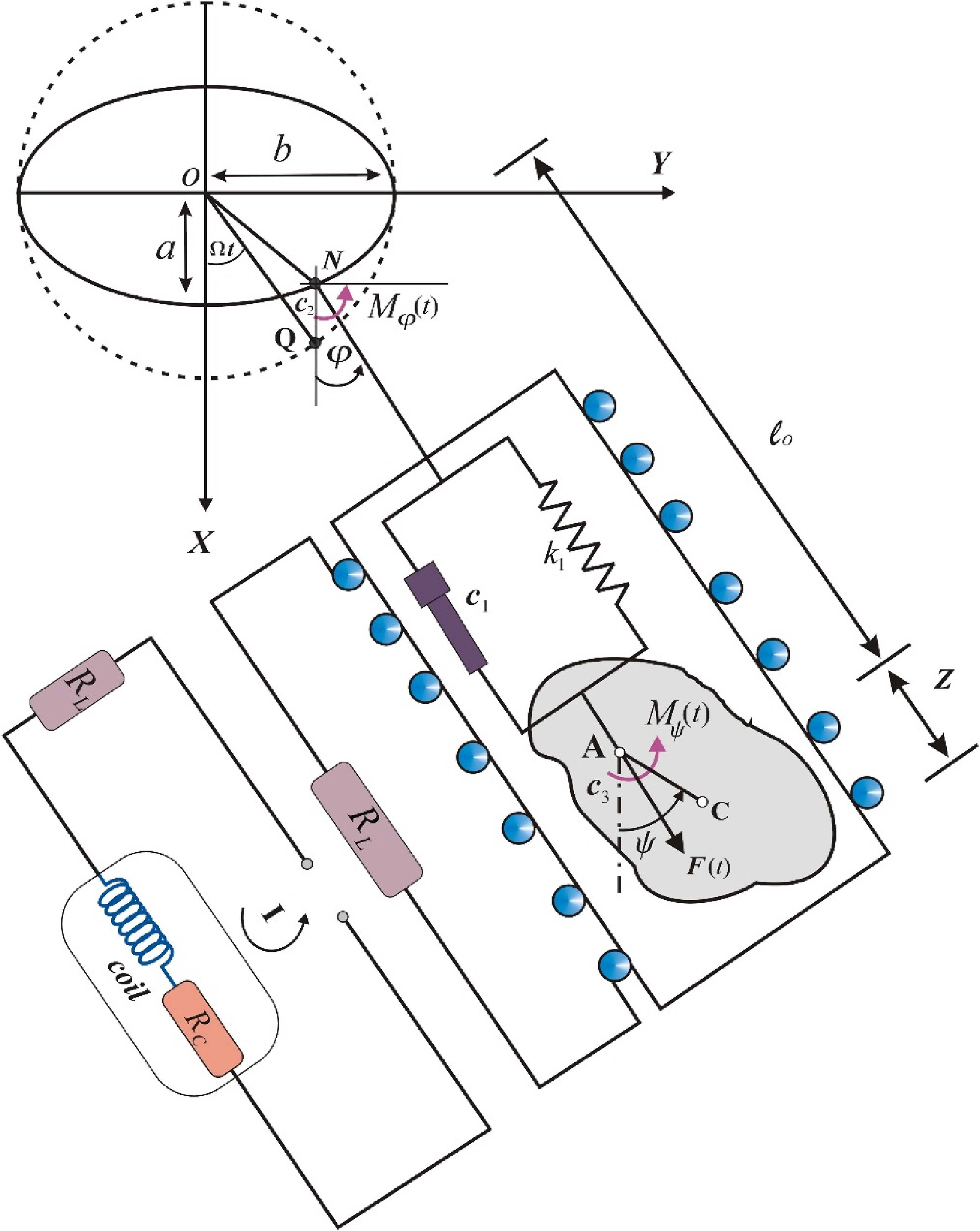
Let’s consider the nonlinear vibrations of a 3DOF dynamical system. Here, we examine the motion of a rigid body constrained to move within a plane, hanging from a point $A$ to one end of a weightless spring possessing a specific stiffness value $k$ . The spring’s other end is fastened to a mobile location $N$ , tracing an elliptical path characterized by major and minor axes denoted by $2 b$ and $2 a$ , respectively. Considering a point $Q$ depicted in Figure (1), which serves as the projection of the moving point $N$ onto an auxiliary circle $b$ and maintaining a steady angular velocity $Ω$ . Hence, the coordinates of $N$ can be formulated after a specific duration of time as follows:

X_{N} = a \cos Ω t, Y_{N} = b \sin Ω t .

(1)

Figure 1.

A schematic diagram of the examined dynamical system.

The rigid body’s characteristics are defined by its mass $m$ , its moment of inertia $U_{A}$ about the axis passing through the point $A$ and perpendicular to the plane’s motion. Point $C$ indicates the body’s center of mass, and the distance $p = AC$ representing its eccentricity. The spring’s damping coefficient is denoted by $C_{1}$ , while $C_{2}$ and $C_{3}$ are the rotatory damping coefficients at the points of rotation $N$ and $A$ , respectively. Considering $l = l_{0} + Z_{s t}$ is the length of the spring at the static equilibrium position after time $t$ , where $l_{0}$ is the spring’s natural length and $Z_{s t} = \frac{m g}{k}$ represents the static elongation, the acceleration due to gravity is denoted as $g$ . All play important roles in the system.

Moreover, the system under study is connected to an electromagnetic device that enables the extraction of electrical power. This is achieved by harnessing the current $I$ generated from the magnet’s oscillations within a coil. The electric component of the harvester is made up of various elements, including the load resistor $R_{L}$ , coil’s inductance $L_{i n d}$ , the resistance of a coil $R_{C}$ , and coil length $L_{c o i l}$ , as shown in Figure (1).

The motion is considered under the influence of harmonic external force $F (t) = F_{0} \cos Ω_{1} t$ , and moments $M_{φ} (t) = M_{1}^{*} \cos Ω_{2} t$ and $M_{ψ} (t) = M_{2}^{*} \cos Ω_{3} t$ . Here, $F_{0}, M_{s}^{*} (s = 1, 2)$ and $Ω_{j} (j = 1, 2, 3)$ are the amplitudes and frequencies of the external force $F (t)$ and the moments $M_{φ} (t), M_{ψ} (t)$ , respectively.

To derive the equations of motion (EOM), we scrutinize the variables representing the spring’s elongation $Z$ , as well as the angular displacements $φ$ and $ψ$ at $N$ and $A$ , respectively.

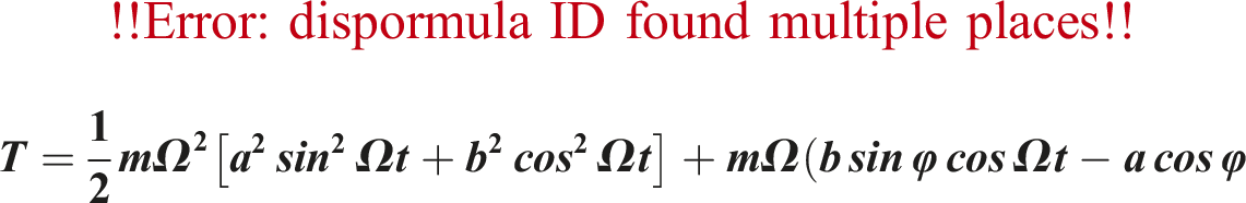
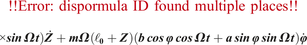
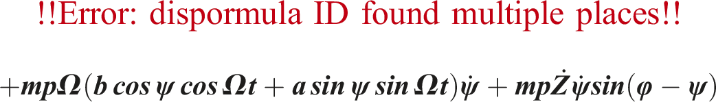
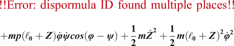
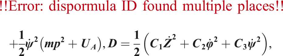
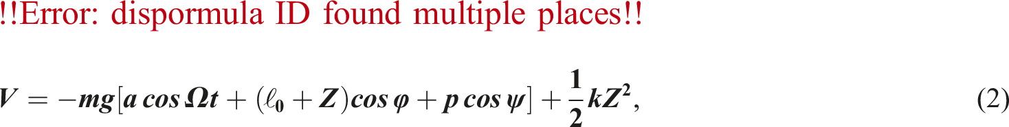
Thus, the system’s kinetic and potential energies are denoted as $T$ and $V$ , along with dissipation’s function $D$ may be expressed as follows

T = \frac{1}{2} m Ω^{2} [a^{2} \sin^{2} Ω t + b^{2} \cos^{2} Ω t] + m Ω (b \sin φ \cos Ω t - a \cos φ

\times \sin Ω t) \dot{Z} + m Ω (ℓ_{0} + Z) (b \cos φ \cos Ω t + a \sin φ \sin Ω t) \dot{φ}

+ m p Ω (b \cos ψ \cos Ω t + a \sin ψ \sin Ω t) \dot{ψ} + m p \dot{Z} \dot{ψ} \sin (φ - ψ)

+ m p (ℓ_{0} + Z) \dot{φ} \dot{ψ} \cos (φ - ψ) + \frac{1}{2} m {\dot{Z}}^{2} + \frac{1}{2} m {(ℓ_{0} + Z)}^{2} {\dot{φ}}^{2}

+ \frac{1}{2} {\dot{ψ}}^{2} (m p^{2} + U_{A}), D = \frac{1}{2} (C_{1} {\dot{Z}}^{2} + C_{2} {\dot{φ}}^{2} + C_{3} {\dot{ψ}}^{2}),

V = - m g [a \cos Ω t + (ℓ_{0} + Z) \cos φ + p \cos ψ] + \frac{1}{2} k Z^{2},

(2)

where the dots represent the rates of change over time

t

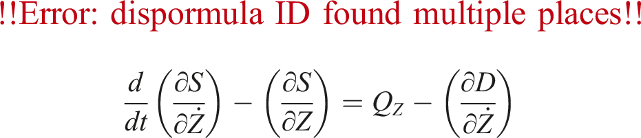
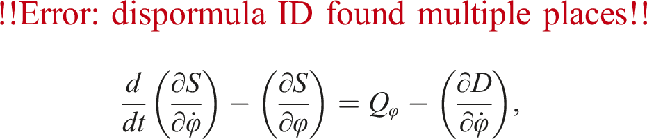
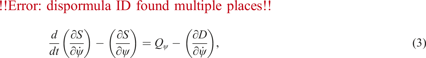
Referring to equation (2), obtaining the Lagrangian $S = T - V$ is straightforward. Subsequently, we can calculate the EOM according to the second kind of Lagrange’s equations⁴⁴ as outlined below

\frac{d}{d t} (\frac{\partial S}{\partial \dot{Z}}) - (\frac{\partial S}{\partial Z}) = Q_{Z} - (\frac{\partial D}{\partial \dot{Z}})

\frac{d}{d t} (\frac{\partial S}{\partial \dot{φ}}) - (\frac{\partial S}{\partial φ}) = Q_{φ} - (\frac{\partial D}{\partial \dot{φ}}),

\frac{d}{d t} (\frac{\partial S}{\partial \dot{ψ}}) - (\frac{\partial S}{\partial ψ}) = Q_{ψ} - (\frac{\partial D}{\partial \dot{ψ}}),

(3)

where

Q_{Z}, Q_{φ},

and

Q_{ψ}

are the generalized forces, which take the forms

Q_{Z} = F (t) = F_{0} \cos Ω_{1} t

Q_{φ} = M_{φ} (t) = M_{1}^{*} \cos Ω_{2} t,

Q_{ψ} = M_{ψ} (t) = M_{2}^{*} \cos Ω_{3} t .

(4)

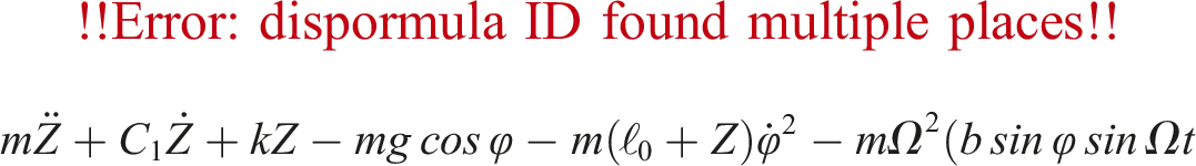
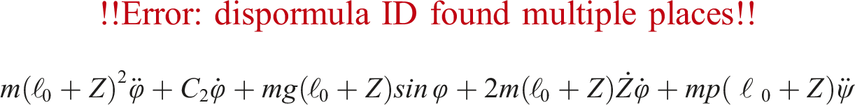
The substitution of (2) and (4) into (3), produces EOM in the form

m \ddot{Z} + C_{1} \dot{Z} + k Z - m g \cos φ - m (ℓ_{0} + Z) {\dot{φ}}^{2} - m Ω^{2} (b \sin φ \sin Ω t

+ a \cos φ \cos Ω t) + m p \ddot{ψ} \sin (φ - ψ) - m p {\dot{ψ}}^{2} \cos (φ - ψ) + B L_{c o i l} Ι = F_{0} \cos Ω_{1} t,

(5)

m {(ℓ_{0} + Z)}^{2} \ddot{φ} + C_{2} \dot{φ} + m g (ℓ_{0} + Z) \sin φ + 2 m (ℓ_{0} + Z) \dot{Z} \dot{φ} + m p (l_{0} + Z) \ddot{ψ}

\times \cos (φ - ψ) + m p (ℓ_{0} + Z) {\dot{ψ}}^{2} \sin (φ - ψ) + m Ω^{2} (ℓ_{0} + Z) (a \sin φ \cos Ω t

- b \cos φ \sin Ω t) = M_{1}^{*} \cos Ω_{2} t,

(6)

\ddot{ψ} (m p^{2} + U_{A}) + C_{3} \dot{ψ} + m g p \sin ψ + \sin (φ - ψ) [m p \ddot{Z} - m p (ℓ_{0} + Z) {\dot{φ}}^{2}]

+ \cos (φ - ψ) [m p (ℓ_{0} + Z) \ddot{φ} + 2 m p \dot{φ} \dot{Z}] + m p Ω^{2} (a \sin ψ \cos Ω t

- b \cos ψ \sin Ω t) = M_{2}^{*} \cos Ω_{3} t,

(7)

By utilizing Kirchhoff’s voltage law and Faraday’s law¹⁸ of electromagnetic induction on the circuit shown in Figure (1), we are able to express the following equation

L_{i n d} \dot{Ι} + R Ι - B L_{c o i l} \dot{Z} = 0,

(8)

where the sum of the coil’s and load’s resistances

R_{C}

and

R_{L}

is represented by

R

and

B

is the magnetic flux density of the magnet.

The below dimensionless parameters may be used to convert the EOM into their dimensionless form

w_{1}^{2} = \frac{k}{m}, w_{2}^{2} = \frac{g}{l}, w_{3}^{2} = \frac{m p g}{U_{A}}, ω_{1} = \frac{w_{1}}{w_{2}}, ω_{2} = \frac{w_{2}}{w_{3}}, ϖ = \frac{Ω}{w_{2}},

s = \frac{p}{l}, p_{1} = \frac{Ω_{1}}{w_{2}}, p_{2} = \frac{Ω_{2}}{w_{2}}, p_{3} = \frac{Ω_{3}}{w_{2}}, γ = \frac{Β^{2} L_{c o i l}^{2}}{m g L_{i n d}} l, α = \frac{R}{L_{i n d} w_{2}},

c_{1} = \frac{C_{1}}{m w_{2}}, c_{2} = \frac{C_{2}}{m w_{2} l^{2}}, c_{3} = \frac{C_{3}}{m w_{2} p l}, f_{1} = \frac{F_{0}}{m g}, f_{2} = \frac{M_{1}^{*}}{m l g},

f_{3} = \frac{M_{2}^{*}}{m p g}, z = \frac{Z - Z_{s t}}{l}, x = \frac{L_{i n d}}{B L_{c o i l} l} Ι, τ = w_{2} t .

(9)

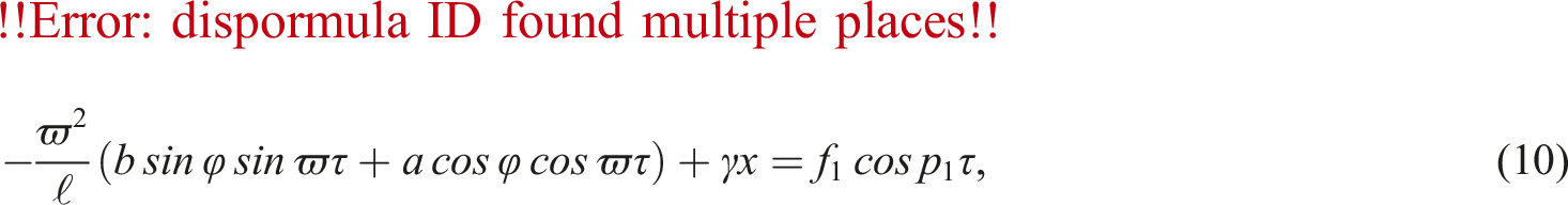
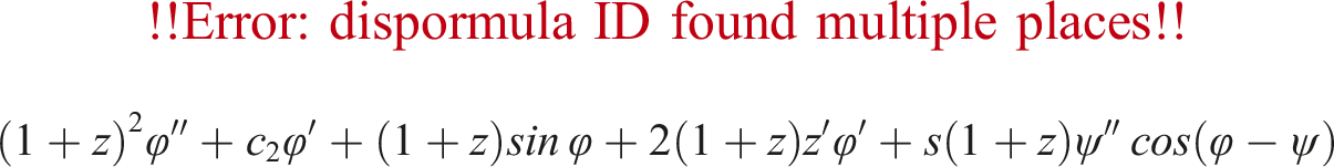
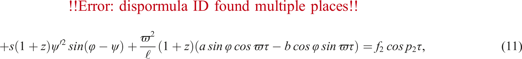
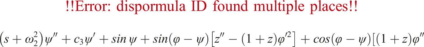
Therefore, the substitution of (9) into (5)-(8) yields the following forms of the EOM

z^{″} + c_{1} z^{'} + ω_{1}^{2} z + (1 - \cos φ) - (1 + z) φ^{' 2} - s ψ^{' 2} \cos (φ - ψ) + s ψ^{″} \sin (φ - ψ)

- \frac{ϖ^{2}}{l} (b \sin φ \sin ϖ τ + a \cos φ \cos ϖ τ) + γ x = f_{1} \cos p_{1} τ,

(10)

{(1 + z)}^{2} φ^{″} + c_{2} φ^{'} + (1 + z) \sin φ + 2 (1 + z) z^{'} φ^{'} + s (1 + z) ψ^{″} \cos (φ - ψ)

+ s (1 + z) ψ^{' 2} \sin (φ - ψ) + \frac{ϖ^{2}}{l} (1 + z) (a \sin φ \cos ϖ τ - b \cos φ \sin ϖ τ) = f_{2} \cos p_{2} τ,

(11)

(s + ω_{2}^{2}) ψ^{″} + c_{3} ψ^{'} + \sin ψ + \sin (φ - ψ) [z^{″} - (1 + z) φ^{' 2}] + \cos (φ - ψ) [(1 + z) φ^{″}

+ 2 z^{'} φ^{'}] + \frac{ϖ^{2}}{l} (a \sin ψ \cos ϖ τ - b \cos ψ \sin ϖ τ) = f_{3} \cos p_{3} τ,

(12)

x^{'} + α x - z^{'} = 0 .

(13)

The prime represent differentiation concerning a variable $τ$ . Equations (10)–(12) are considered nonlinear second-order ordinary differential equations (ODE).

It must be noted that in energy harvesting systems, continuous physical force is crucial for generating electricity efficiently. Here’s an explanation of how this force works and its role in energy harvesters:

Energy harvesters convert mechanical energy from physical forces into electrical energy. This process relies on a continuous external force to maintain the motion required for energy conversion. Many harvesters utilize vibrational forces, such as the motion of a vibrating rigid body. For instance, an electromagnetic device might be attached to a vibrating structure, as seen in Figure (1). To continuously generate electricity, the harvester must maintain consistent motion. For vibrational energy harvesters, this means that the vibrating source must produce ongoing oscillations according to the rotational harmonic moments at the points $O$ and $A$ , and the harmonic physical force $F (t)$ in the spring’s direction. The applied force and moments cause the harvester (e.g., a mass-spring system in the electromagnetic harvester) to oscillate or vibrate.

Perturbation methodology

The primary goal of this section is to acquire the sought-after asymptotic solutions to the EOMs outlined in the provided system (10)-(13), specifically targeting up to the third-order of approximation. This will be achieved by leveraging the MST as a crucial perturbation technique. Furthermore, the systems’ resonance cases⁴⁵ will be categorized. To achieve this, we will employ Taylor series expansion to approximate the trigonometric functions in $φ$ and $ψ$ , as well as their derivatives up to the third-order, which is applicable in the vicinity of the static equilibrium position. Consequently, equations describing the system can be reformulated accordingly.

z^{″} + c_{1} z^{'} + ω_{1}^{2} z + \frac{φ^{2}}{2} - (1 + z) φ^{' 2} - \frac{s}{36} [φ ψ (φ^{2} - 6) (ψ^{2} - 6) + 9 (φ^{2} - 2) (ψ^{2} - 2)] ψ^{' 2}

+ \frac{s}{12} [φ (φ^{2} - 6) (ψ^{2} - 2) - ψ (φ^{2} - 2) (ψ^{2} - 6)] ψ^{″} + \frac{ϖ^{2}}{l} [b (\frac{φ^{3}}{6} - φ) \sin ϖ τ

+ a (\frac{φ^{2}}{2} - 1) \cos ϖ τ] + γ x = f_{1} \cos p_{1} τ,

(14)

{(z + 1)}^{2} φ^{″} + c_{2} φ^{'} + (1 + z) (φ - \frac{φ^{3}}{6}) + 2 (1 + z) z^{'} φ^{'} + \frac{s}{36} (1 + z) [φ ψ (φ^{2} - 6) (ψ^{2} - 6)

+ 9 (φ^{2} - 2) (ψ^{2} - 2)] ψ^{″} + \frac{s}{12} (1 + z) [φ (φ^{2} - 6) (ψ^{2} - 2) - ψ (φ^{2} - 2) (ψ^{2} - 6)] ψ^{' 2}

+ \frac{ϖ^{2}}{l} (1 + z) [b (\frac{φ^{2}}{2} - 1) \sin ϖ τ - a (\frac{φ^{3}}{6} - φ) \cos ϖ τ] = f_{2} \cos p_{2} τ,

(15)

(s + ω_{2}^{2}) ψ^{″} + c_{3} ψ^{'} + (ψ - \frac{ψ^{3}}{6}) - \frac{1}{12} (1 + z) [φ (φ^{2} - 6) (ψ^{2} - 2) - ψ (φ^{2} - 2) (ψ^{2} - 6)] φ^{' 2}

+ \frac{1}{36} (1 + z) [φ ψ (φ^{2} - 6) (ψ^{2} - 6) + 9 (φ^{2} - 2) (ψ^{2} - 2)] φ^{″} + \frac{1}{18} [φ ψ (φ^{2} - 6) (ψ^{2} - 6)

+ 9 (φ^{2} - 2) (ψ^{2} - 2)] z^{'} φ^{'} + \frac{1}{12} [φ (φ^{2} - 6) (ψ^{2} - 2) - ψ (φ^{2} - 2) (ψ^{2} - 6)] z^{″} + \frac{ϖ^{2}}{l} \times

[b (\frac{ψ^{2}}{2} - 1) \sin ϖ τ - a (\frac{ψ^{3}}{6} - ψ) \cos ϖ τ] = f_{3} \cos p_{3} τ,

(16)

x^{'} + α x - z^{'} = 0 .

(17)

It is assumed that the generalized coordinates might be represented in relation to the order $0 < ε ≪ 1$ . Hence, new variables $y, ϕ, ζ,$ and $χ$ are taken into consideration in the following manner:

z (τ) = ε y (τ; ε), φ (τ) = ε ϕ (τ; ε), ψ (τ) = ε ζ (τ; ε), x (τ) = ε χ (τ; ε) .

(18)

According to MST, we can present the function $y, ϕ, ζ,$ and $χ$ in terms of powers of $ε$ in the following manner⁴⁶:

y = \sum_{k = 0}^{2} ε^{k} y_{k + 1} (τ_{0}, τ_{1}, τ_{2}) + O (ε^{3}),

ϕ = \sum_{k = 0}^{2} ε^{k} ϕ_{k + 1} (τ_{0}, τ_{1}, τ_{2}) + O (ε^{3}),

ζ = \sum_{k = 0}^{2} ε^{k} ζ_{k + 1} (τ_{0}, τ_{1}, τ_{2}) + O (ε^{3})

χ = \sum_{k = 0}^{2} ε^{k} χ_{k + 1} (τ_{0}, τ_{1}, τ_{2}) + O (ε^{3}),

(19)

where

τ_{n} = ε^{n} τ (n = 0, 1, 2)

perform different time scales, in which

τ_{0}

and

τ_{1}, τ_{2}

act as the fast and slow time scales, respectively. In order to establish functions

y, ϕ, ζ,

and

χ

based on

τ_{n}

, we convert

τ

τ_{n}

using specific operators⁴⁷

\frac{d}{d τ} = \frac{\partial}{\partial τ_{0}} + ε \frac{\partial}{\partial τ_{1}} + ε^{2} \frac{\partial}{\partial τ_{2}},

\frac{d^{2}}{d τ^{2}} = \frac{\partial^{2}}{\partial τ_{0}^{2}} + 2 ε \frac{\partial^{2}}{\partial τ_{0} \partial τ_{1}} + ε^{2} (\frac{\partial^{2}}{\partial τ_{1}^{2}} + 2 \frac{\partial^{2}}{\partial τ_{0} \partial τ_{2}}) + O (ε^{3}) .

(20)

It’s crucial to acknowledge that terms of $O (ε^{3})$ and beyond are deemed insignificant due to their comparatively small magnitudes.

The eccentricity, the damping coefficients, and generalized forces can be represented in terms of $ε$ as shown below:

a = ε^{2} \tilde{a}, b = ε^{2} \tilde{b}, s = ε^{2} \tilde{s}, γ = ε^{2} \tilde{γ},

α = \tilde{α}, c_{j} = ε^{2} {\tilde{c}}_{j}, f_{j} = ε^{3} {\tilde{f}}_{j}, (j = 1, 2, 3)

(21)

where the parameters

\tilde{a}, \tilde{b}, \tilde{s}, \tilde{γ}, \tilde{α}, {\tilde{c}}_{j},

and

{\tilde{f}}_{j}

are of order 1.

Inserting equations (18)–(21) into equations (14)–(17) and subsequently comparing the coefficients of the same powers of $ε, ε^{2}$ and $ε^{3}$ , we can derive the below three distinct sets of partial differential equations (PDEs):Order of $ε$

\frac{\partial^{2} y_{1}}{\partial τ_{0}^{2}} + ω_{1}^{2} y_{1} = 0,

(22)

\frac{\partial^{2} ϕ_{1}}{\partial τ_{0}^{2}} + ϕ_{1} = 0,

(23)

\frac{\partial^{2} ζ_{1}}{\partial τ_{0}^{2}} + \frac{1}{ω_{2}^{2}} ζ_{1} = - \frac{1}{ω_{2}^{2}} \frac{\partial^{2} ϕ_{1}}{\partial τ_{0}^{2}},

(24)

\frac{\partial χ_{1}}{\partial τ_{0}} + \tilde{α} χ_{1} = \frac{\partial y_{1}}{\partial τ_{0}} .

(25)

Order of

ε^{2}

\frac{\partial^{2} y_{2}}{\partial τ_{0}^{2}} + ω_{1}^{2} y_{2} = \frac{ϖ^{2}}{l} \tilde{a} \cos (ϖ τ_{0}) - 2 \frac{\partial^{2} y_{1}}{\partial τ_{0} τ_{1}} + {(\frac{\partial ϕ_{1}}{\partial τ_{0}})}^{2} - \frac{1}{2} {ϕ_{1}}^{2},

(26)

\frac{\partial^{2} ϕ_{2}}{\partial τ_{0}^{2}} + ϕ_{2} = \frac{ϖ^{2}}{l} \tilde{b} \sin (ϖ τ_{0}) - 2 [\frac{\partial^{2} ϕ_{1}}{\partial τ_{0} \partial τ_{1}} + y_{1} \frac{\partial^{2} ϕ_{1}}{\partial τ_{0}^{2}} + \frac{\partial y_{1}}{\partial τ_{0}} \frac{\partial ϕ_{1}}{\partial τ_{0}}] - y_{1} ϕ_{1},

(27)

\frac{\partial^{2} ζ_{2}}{\partial τ_{0}^{2}} + \frac{1}{ω_{2}^{2}} ζ_{2} = \frac{ϖ^{2}}{l ω_{2}^{2}} \tilde{b} \sin (ϖ τ_{0}) - 2 \frac{\partial^{2} ζ_{1}}{\partial τ_{0} \partial τ_{1}} - \frac{2}{ω_{2}^{2}} (\frac{\partial^{2} ϕ_{1}}{\partial τ_{0} \partial τ_{1}} + \frac{\partial y_{1}}{\partial τ_{0}} \frac{\partial ϕ_{1}}{\partial τ_{0}})

+ \frac{1}{ω_{2}^{2}} (ζ_{1} \frac{\partial^{2} y_{1}}{\partial τ_{0}^{2}} - ϕ_{1} \frac{\partial^{2} y_{1}}{\partial τ_{0}^{2}} - y_{1} \frac{\partial^{2} ϕ_{1}}{\partial τ_{0}^{2}}) - \frac{1}{ω_{2}^{2}} \frac{\partial^{2} ϕ_{2}}{\partial τ_{0}^{2}},

(28)

\frac{\partial χ_{2}}{\partial τ_{0}} + \tilde{α} χ_{2} = \frac{\partial y_{2}}{\partial τ_{0}} - \frac{\partial χ_{1}}{\partial τ_{1}} + \frac{\partial y_{1}}{\partial τ_{1}} .

(29)

Order of

ε^{3}

\frac{\partial^{2} y_{3}}{\partial τ_{0}^{2}} + ω_{1}^{2} y_{3} = {\tilde{f}}_{1} \cos (p_{1} τ_{0}) + \frac{ϖ^{2}}{l} \tilde{b} ϕ_{1} \sin (ϖ τ_{0}) - \frac{\partial^{2} y_{1}}{\partial τ_{1}^{2}}

- 2 (\frac{\partial^{2} y_{1}}{\partial τ_{0} \partial τ_{2}} + \frac{\partial^{2} y_{2}}{\partial τ_{0} \partial τ_{1}}) + 2 (\frac{\partial ϕ_{1}}{\partial τ_{0}} \frac{\partial ϕ_{2}}{\partial τ_{0}} + \frac{\partial ϕ_{1}}{\partial τ_{0}} \frac{\partial ϕ_{1}}{\partial τ_{1}})

+ y_{1} {(\frac{\partial ϕ_{1}}{\partial τ_{0}})}^{2} - {\tilde{c}}_{1} \frac{\partial y_{1}}{\partial τ_{0}} - ϕ_{1} ϕ_{2} - \tilde{γ} χ_{1},

(30)

\frac{\partial^{2} ϕ_{3}}{\partial τ_{0}^{2}} + ϕ_{3} = {\tilde{f}}_{2} \cos (p_{2} τ_{0}) - \frac{ϖ^{2}}{l} \tilde{a} ϕ_{1} \cos (ϖ τ_{0}) + \frac{ϖ^{2}}{l} \tilde{b} y_{1} \sin (ϖ τ_{0})

- 2 (\frac{\partial^{2} ϕ_{1}}{\partial τ_{0} \partial τ_{2}} + \frac{\partial^{2} ϕ_{2}}{\partial τ_{0} \partial τ_{1}}) - 2 (y_{1} \frac{\partial^{2} ϕ_{2}}{\partial τ_{0}^{2}} + y_{2} \frac{\partial^{2} ϕ_{1}}{\partial τ_{0}^{2}}) - 4 y_{1} \frac{\partial^{2} ϕ_{1}}{\partial τ_{0} \partial τ_{1}}

- 2 y_{1} \frac{\partial ϕ_{1}}{\partial τ_{0}} \frac{\partial y_{1}}{\partial τ_{0}} - 2 (\frac{\partial ϕ_{2}}{\partial τ_{0}} \frac{\partial y_{1}}{\partial τ_{0}} + \frac{\partial ϕ_{1}}{\partial τ_{0}} \frac{\partial y_{1}}{\partial τ_{1}} + \frac{\partial ϕ_{1}}{\partial τ_{0}} \frac{\partial y_{2}}{\partial τ_{0}} + \frac{\partial ϕ_{1}}{\partial τ_{1}} \frac{\partial y_{1}}{\partial τ_{0}})

- y_{1} ϕ_{2} - y_{2} ϕ_{1} - y_{1}^{2} \frac{\partial^{2} ϕ_{1}}{\partial {τ_{0}}^{2}} - {\tilde{c}}_{2} \frac{\partial ϕ_{1}}{\partial τ_{0}} + \frac{1}{6} ϕ_{1}^{3} - \frac{\partial^{2} ϕ_{1}}{\partial τ_{1}^{2}} - \tilde{s} \frac{\partial^{2} ζ_{1}}{\partial τ_{0}^{2}},

(31)

\frac{\partial^{2} ζ_{3}}{\partial τ_{0}^{2}} + \frac{1}{ω_{2}^{2}} ζ_{3} = \frac{{\tilde{f}}_{3}}{ω_{2}^{2}} \cos (p_{3} τ_{0}) - \frac{ϖ^{2}}{l ω_{2}^{2}} \tilde{a} ζ_{1} \cos (ϖ τ_{0}) - 2 (\frac{\partial^{2} ζ_{1}}{\partial τ_{0} \partial τ_{2}} + \frac{\partial^{2} ζ_{2}}{\partial τ_{0} \partial τ_{1}})

- \frac{\partial^{2} ζ_{1}}{\partial τ_{1}^{2}} - \frac{1}{ω_{2}^{2}} \frac{\partial^{2} ϕ_{1}}{\partial τ_{1}^{2}} - \frac{1}{ω_{2}^{2}} \frac{\partial^{2} ϕ_{3}}{\partial τ_{0}^{2}} - \frac{{\tilde{c}}_{3}}{ω_{2}^{2}} \frac{\partial ζ_{1}}{\partial τ_{0}} - \frac{\tilde{s}}{ω_{2}^{2}} \frac{\partial^{2} ζ_{1}}{\partial τ_{0}^{2}} + \frac{1}{6 ω_{2}^{2}} ζ_{1}^{3}

- \frac{1}{ω_{2}^{2}} (ϕ_{1} \frac{\partial^{2} y_{2}}{\partial τ_{0}^{2}} + ϕ_{2} \frac{\partial^{2} y_{1}}{\partial τ_{0}^{2}} - ζ_{1} \frac{\partial^{2} y_{2}}{\partial τ_{0}^{2}} - ζ_{2} \frac{\partial^{2} y_{1}}{\partial {τ_{0}}^{2}} + y_{1} \frac{\partial^{2} ϕ_{2}}{\partial {τ_{0}}^{2}} + y_{2} \frac{\partial^{2} ϕ_{1}}{\partial {τ_{0}}^{2}})

- \frac{2}{ω_{2}^{2}} (\frac{\partial^{2} ϕ_{1}}{\partial τ_{0} \partial τ_{2}} + \frac{\partial^{2} ϕ_{2}}{\partial τ_{0} \partial τ_{1}}) - \frac{2}{ω_{2}^{2}} (ϕ_{1} \frac{\partial^{2} y_{1}}{\partial τ_{0} \partial τ_{1}} + y_{1} \frac{\partial^{2} ϕ_{1}}{\partial τ_{0} \partial τ_{1}} - ζ_{1} \frac{\partial^{2} y_{1}}{\partial τ_{0} \partial τ_{1}})

- \frac{2}{ω_{2}^{2}} (\frac{\partial ϕ_{2}}{\partial τ_{0}} \frac{\partial y_{1}}{\partial τ_{0}} + \frac{\partial ϕ_{1}}{\partial τ_{0}} \frac{\partial y_{2}}{\partial τ_{0}} + \frac{\partial ϕ_{1}}{\partial τ_{0}} \frac{\partial y_{1}}{\partial τ_{1}} + \frac{\partial ϕ_{1}}{\partial τ_{1}} \frac{\partial y_{1}}{\partial τ_{0}}) + \frac{1}{ω_{2}^{2}} ϕ_{1} {(\frac{\partial ϕ_{1}}{\partial τ_{0}})}^{2}

- \frac{1}{ω_{2}^{2}} ζ_{1} {(\frac{\partial ϕ_{1}}{\partial τ_{0}})}^{2} - \frac{1}{ω_{2}^{2}} ζ_{1} ϕ_{1} \frac{\partial^{2} ϕ_{1}}{\partial τ_{0}^{2}} + \frac{1}{2 ω_{2}^{2}} (ζ_{1}^{2} \frac{\partial^{2} ϕ_{1}}{\partial {τ_{0}}^{2}} + ϕ_{1}^{2} \frac{\partial^{2} ϕ_{1}}{\partial {τ_{0}}^{2}}),

(32)

\frac{\partial χ_{3}}{\partial τ_{0}} + \tilde{α} χ_{3} = \frac{\partial y_{3}}{\partial τ_{0}} - (\frac{\partial χ_{2}}{\partial τ_{1}} + \frac{\partial χ_{1}}{\partial τ_{2}}) + \frac{\partial y_{2}}{\partial τ_{1}} + \frac{\partial y_{1}}{\partial τ_{2}} .

(33)

It’s worth noting that the three systems of order of $ε$ create a total of PDEs that can be solved one after the other. In order to accomplish this task, let’s begin with equations (22)–(25), which possess the following general solutions:

y_{1} = A_{1} e^{i ω_{1} τ_{0}} + {\bar{A}}_{1} e^{- i ω_{1} τ_{0}},

(34)

ϕ_{1} = A_{2} e^{i τ_{0}} + {\bar{A}}_{2} e^{- i τ_{0}},

(35)

ζ_{1} = A_{3} e^{\frac{i τ_{0}}{ω_{2}}} + {\bar{A}}_{3} e^{\frac{- i τ_{0}}{ω_{2}}} + \frac{1}{(1 - ω_{2}^{2})} (A_{2} e^{i τ_{0}} + {\bar{A}}_{2} e^{- i τ_{0}}),

(36)

where

A_{j} = A_{j} (τ_{1}, τ_{2}) (j = 1, 2, 3)

are unidentified complex functions, while

\bar{A_{j}}

indicate their complex conjugates.

In order to find the overall solution of $χ_{1}$ , substituting equation (34) into equation (25) to derive a nonhomogeneous PDE that can be solved using a specific form

χ_{1} = B_{1} e^{- α τ_{0}} + i ω_{1} [\frac{A_{1}}{(α + i ω_{1})} e^{i ω_{1} τ_{0}} - \frac{{\bar{A}}_{1}}{(α - i ω_{1})} e^{- i ω_{1} τ_{0}}]; i = \sqrt{- 1},

(37)

where, the definition of

B_{1}

mirror the previous definition of

A_{j}

Inserting equations (34)-(37) into (26)-(29) and eliminating terms resulting in secular behavior, we can derive a consistent asymptotic second-order of solutions as follows:

y_{2} = - \frac{3 A_{2}^{2}}{2 (ω_{1}^{2} - 4)} e^{2 i τ_{0}} + \frac{ϖ^{2} \tilde{a}}{2 l (ω_{1}^{2} - ϖ^{2})} e^{i ϖ τ_{0}} + \frac{1}{ω_{1}^{2}} A_{2} {\bar{A}}_{2} + C C,

(38)

ϕ_{2} = - \frac{(1 + 2 ω_{1})}{ω_{1} (2 + ω_{1})} A_{1} A_{2} e^{i (1 + ω_{1}) τ_{0}} + \frac{(1 - 2 ω_{1})}{ω_{1} (2 - ω_{1})} {\bar{A}}_{1} A_{2} e^{i (1 - ω_{1}) τ_{0}} - \frac{i ϖ^{2} \tilde{b}}{2 l (1 - ϖ^{2})} e^{i ϖ τ_{0}} + C C,

(39)

ζ_{2} = \frac{1 + 2 ω_{1} + (ω_{1} - 1) {(ω_{1} + 1)}^{3} ω_{2}^{2}}{ω_{1} (ω_{1} + 2) (ω_{2}^{2} - 1) [1 - ω_{2}^{2} {(1 + ω_{1})}^{2}]} A_{1} A_{2} e^{i (1 + ω_{1}) τ_{0}} + {\bar{A}}_{1} A_{2} e^{i (1 - ω_{1}) τ_{0}}

\times \frac{1 - 2 ω_{1} + (ω_{1} + 1) {(ω_{1} - 1)}^{3} ω_{2}^{2}}{ω_{1} (ω_{1} - 2) (ω_{2}^{2} - 1) [1 - ω_{2}^{2} {(1 - ω_{1})}^{2}]} - \frac{ω_{1}^{2}}{[1 - {(1 + ω_{1} ω_{2})}^{2}]} A_{1} A_{3} e^{i (\frac{1 + ω_{1} ω_{2}}{ω_{2}}) τ_{0}}

- \frac{ω_{1}^{2}}{[1 - {(1 - ω_{1} ω_{2})}^{2}]} {\bar{A}}_{1} A_{3} e^{i (\frac{1 - ω_{1} ω_{2}}{ω_{2}}) τ_{0}} - \frac{i ϖ^{2} \tilde{b}}{2 l (1 - ϖ^{2}) (1 - ϖ^{2} ω_{2}^{2})} e^{i ϖ τ_{0}} + C C,

(40)

χ_{2} = - \frac{3 i}{(α + 2 i) (ω_{1}^{2} - 4)} A_{2}^{2} e^{2 i τ_{0}} + \frac{i ϖ^{3} \tilde{a}}{2 l (ω_{1}^{2} - ϖ^{2}) (α + i ϖ)} e^{i ϖ τ_{0}} + C C,

(41)

where

C C

represents the preceding terms’ conjugate.

Based on the provided information, it is possible to establish the criteria of second-order approximations for eliminating secular terms as in the following specified forms:

\frac{\partial A_{1}}{\partial τ_{1}} = 0, \frac{\partial A_{2}}{\partial τ_{1}} = 0, \frac{\partial A_{3}}{\partial τ_{1}} = 0, \frac{\partial B_{1}}{\partial τ_{1}} = 0 .

(42)

Hence, $A_{j} = A_{j} (τ_{2})$ and $B_{1} = B_{1} (τ_{2})$ .

Making use of equations (34)–(37) and (38)-(42) into (30)-(33), the third-order approximate solutions can be expressed through the elimination of terms that lead to secular ones. To eliminate these terms, certain conditions need to be met

2 i ω_{1} \frac{\partial A_{1}}{\partial τ_{2}} + A_{1} [i {\tilde{c}}_{1} ω_{1} + \frac{i \tilde{γ} ω_{1}}{(α + i ω_{1})} + \frac{6 (ω_{1}^{2} - 1)}{(ω_{1}^{2} - 4)} A_{2} {\bar{A}}_{2}] = 0,

(43)

2 i \frac{\partial A_{2}}{\partial τ_{2}} + A_{2} [i {\tilde{c}}_{2} - \frac{\tilde{s}}{(1 - ω_{2}^{2})} + \frac{6 (ω_{1}^{2} - 1)}{(ω_{1}^{2} - 4)} A_{1} {\bar{A}}_{1} - \frac{ω_{1}^{4} + 7 ω_{1}^{2} - 8}{2 ω_{1}^{2} (ω_{1}^{2} - 4)} A_{2} {\bar{A}}_{2}] = 0,

(44)

\frac{2 i}{ω_{2}} \frac{\partial A_{3}}{\partial τ_{2}} + A_{3} [\frac{i {\tilde{c}}_{3}}{ω_{2}^{3}} - \frac{\tilde{s}}{ω_{2}^{2} (ω_{2}^{2} - 1)} - \frac{1}{2 ω_{2}^{2}} A_{3} {\bar{A}}_{3} + \frac{(1 - 2 ω_{2}^{2})}{ω_{2}^{2} {(1 - ω_{2}^{2})}^{2}} A_{2} {\bar{A}}_{2}

- \frac{2 ω_{1}^{4}}{ω_{2}^{2} (4 - ω_{1}^{2} ω_{2}^{2})} A_{1} {\bar{A}}_{1}] = 0,

(45)

\frac{\partial B_{1}}{\partial τ_{2}} - \frac{α \tilde{γ} B_{1}}{(α^{2} + ω_{1}^{2})} = 0 .

(46)

Subsequently, the solutions of the third approximations

y_{3}, ϕ_{3}, ζ_{3}

, and

χ_{3}

assume the following forms:

y_{3} = \frac{{\tilde{f}}_{1} e^{i p_{1} τ_{0}}}{2 (ω_{1}^{2} - p_{1}^{2})} + \frac{i ϖ^{3} (ϖ + 2) \tilde{b} A_{2} e^{i (ϖ + 1) τ_{0}}}{2 l [ω_{1}^{2} - {(ϖ + 1)}^{2}] (1 - ϖ^{2})} + \frac{i ϖ^{3} (ϖ - 2) \tilde{b} {\bar{A}}_{2} e^{i (ϖ - 1) τ_{0}}}{2 l [ω_{1}^{2} - {(ϖ - 1)}^{2}] (1 - ϖ^{2})}

- \frac{3 (ω_{1} + 1) A_{1} A_{2}^{2} e^{i (2 + ω_{1}) τ_{0}}}{4 ω_{1} (ω_{1} + 2)} + \frac{3 (ω_{1} - 1) {\bar{A}}_{1} A_{2}^{2} e^{i (2 - ω_{1}) τ_{0}}}{4 ω_{1} (ω_{1} - 2)} - \frac{\tilde{γ} B_{1} e^{- α τ_{0}}}{(α^{2} + ω_{1}^{2})} + C C,

(47)

ϕ_{3} = \frac{{\tilde{f}}_{2} e^{i p_{2} τ_{0}}}{2 (1 - p_{2}^{2})} - \frac{(ω_{1}^{2} - 49) A_{2}^{3} e^{3 i τ_{0}}}{48 (ω_{1}^{2} - 4)} + \frac{\tilde{s} A_{3} e^{(\frac{i}{ω_{2}}) τ_{0}}}{(ω_{2}^{2} - 1)} - \frac{i ϖ^{3} \tilde{b} (2 ω_{1} + ϖ) A_{1} e^{i (ϖ + ω_{1}) τ_{0}}}{2 l (1 - ϖ^{2}) (1 - {(ϖ + ω_{1})}^{2})}

+ \frac{i ϖ^{3} \tilde{b} (2 ω_{1} - ϖ) {\bar{A}}_{1} e^{i (ϖ - ω_{1}) τ_{0}}}{2 l (1 - ϖ^{2}) (1 - {(ϖ - ω_{1})}^{2})} - \frac{ϖ \tilde{a} (1 + 2 ϖ + ϖ^{2} - ω_{1}^{2}) A_{2} e^{i (ϖ + 1) τ_{0}}}{2 l (ω_{1}^{2} - ϖ^{2}) (2 + ϖ)}

+ \frac{ϖ \tilde{a} (1 - 2 ϖ + ϖ^{2} - ω_{1}^{2}) {\bar{A}}_{2} e^{i (ϖ - 1) τ_{0}}}{2 l (ω_{1}^{2} - ϖ^{2}) (2 - ϖ)} + \frac{(6 ω_{1}^{3} + 11 ω_{1}^{2} + 6 ω_{1} + 1) A_{1}^{2} A_{2} e^{i (1 + 2 ω_{1}) τ_{0}}}{4 ω_{1}^{2} (ω_{1} + 2) (1 + ω_{1})}

+ \frac{(6 ω_{1}^{3} - 11 ω_{1}^{2} + 6 ω_{1} - 1) {\bar{A}}_{1}^{2} A_{2} e^{i (1 - 2 ω_{1}) τ_{0}}}{4 ω_{1}^{2} (ω_{1} - 2) (1 - ω_{1})} + C C,

(48)

ζ_{3} = \frac{{\tilde{f}}_{3} e^{i p_{3} τ_{0}}}{2 (1 - ω_{2}^{2} p_{3}^{2})} + \frac{p_{2}^{2} {\tilde{f}}_{2} e^{i p_{2} τ_{0}}}{2 (1 - p_{2}^{2}) (1 - ω_{2}^{2} p_{2}^{2})} - \frac{A_{3}^{3}}{48} e^{(\frac{3 i}{ω_{2}}) τ_{0}} + E_{1} A_{2}^{3} e^{3 i τ_{0}} + E_{2} A_{2} e^{i τ_{0}}

+ E_{3} A_{2}^{2} A_{3} e^{i (\frac{2 ω_{2} + 1}{ω_{2}}) τ_{0}} + E_{4} A_{2}^{2} {\bar{A}}_{3} e^{i (\frac{2 ω_{2} - 1}{ω_{2}}) τ_{0}} + E_{5} A_{2} A_{3}^{2} e^{i (\frac{ω_{2} + 2}{ω_{2}}) τ_{0}} + E_{6} A_{2} {\bar{A}}_{3}^{2} e^{i (\frac{ω_{2} - 2}{ω_{2}}) τ_{0}}

+ E_{7} A_{2} e^{i (ϖ + 1) τ_{0}} + E_{8} {\bar{A}}_{2} e^{i (ϖ - 1) τ_{0}} - E_{9} A_{1}^{2} A_{2} e^{i (1 + 2 ω_{1}) τ_{0}} - E_{10} {\bar{A}}_{1}^{2} A_{2} e^{i (1 - 2 ω_{1}) τ_{0}}

+ E_{11} A_{1} e^{i (ϖ + ω_{1}) τ_{0}} + E_{12} {\bar{A}}_{1} e^{i (ϖ - ω_{1}) τ_{0}} + E_{13} A_{3} e^{i (\frac{ϖ ω_{2} + 1}{ω_{2}}) τ_{0}} + E_{14} {\bar{A}}_{3} e^{i (\frac{ϖ ω_{2} - 1}{ω_{2}}) τ_{0}}

+ E_{15} A_{1}^{2} A_{3} e^{i (\frac{1 + 2 ω_{1} ω_{2}}{ω_{2}}) τ_{0}} + E_{16} {\bar{A}}_{1}^{2} A_{3} e^{i (\frac{1 - 2 ω_{1} ω_{2}}{ω_{2}}) τ_{0}} + C C,

(49)

where

E_{υ} (υ = 1, 2, . . ., 16)

can be obtained easily (see Appendix I).

χ_{3} = \frac{i p_{1} {\tilde{f}}_{1} e^{i p_{1} τ_{0}}}{2 (ω_{1}^{2} - p_{1}^{2}) (α + i p_{1})} + \frac{A_{1} e^{i ω_{1} τ_{0}}}{(α + i ω_{1})} [1 - \frac{i ω_{1}}{(α + i ω_{1})}] [- \frac{{\tilde{c}}_{1}}{2} - \frac{\tilde{γ}}{2 (α + i ω_{1})}

+ \frac{3 i (ω_{1}^{2} - 1)}{ω_{1} (ω_{1}^{2} - 4)} A_{2} {\bar{A}}_{2}] - \frac{ϖ^{3} \tilde{b} (ϖ + 2) A_{2} e^{i (ϖ + 1) τ_{0}}}{2 l (1 - ϖ) [ω_{1}^{2} - {(ϖ + 1)}^{2}] [α + i (ϖ + 1)]}

+ \frac{ϖ^{3} \tilde{b} (ϖ - 2) {\bar{A}}_{2} e^{i (ϖ - 1) τ_{0}}}{2 l (ϖ + 1) [ω_{1}^{2} - {(ϖ - 1)}^{2}] [α + i (ϖ - 1)]} + \frac{3 i {(ω_{1} + 1)}^{2} A_{1} A_{2}^{2} e^{i (2 + ω_{1}) τ_{0}}}{ω_{1} [ω_{1}^{2} - {(2 + ω_{1})}^{2}] [α + i (2 + ω_{1})]}

- \frac{3 i {(ω_{1} - 1)}^{2} {\bar{A}}_{1} A_{2}^{2} e^{i (2 - ω_{1}) τ_{0}}}{ω_{1} [ω_{1}^{2} - {(2 - ω_{1})}^{2}] [α + i (2 - ω_{1})]} + C C .

(50)

Now, we can go back to determine the functions $A_{j}$ and $B_{1}$ by applying the elimination criteria for secular terms (42)-(46), in addition to the specified initial conditions.

z (0) = η_{01}, φ (0) = η_{03}, ψ (0) = η_{05}, x (0) = η_{07},

z^{'} (0) = η_{02}, φ^{'} (0) = η_{04}, ψ^{'} (0) = η_{06},

(51)

where

η_{01}, η_{02}, . . ., η_{07}

are known quantities.

It must be noted that approximate solutions can provide insights into the behavior of complex systems without the need for overly complex mathematical analysis. Even if an exact solution is not feasible, approximate solutions can help us understand the system’s response to various inputs and initial conditions. These solutions can be used to validate analytical models developed for vibrating dynamical systems, predict the behavior of vibrating dynamical systems, and make timely adjustments to optimize performance or prevent failures. By providing insights into the behavior of vibrating dynamical systems under different conditions, it can help assess the risks associated with system failures or performance degradation. This is particularly important in safety-critical applications such as aerospace or automotive engineering.

Resonance scenarios and stability assessment

In this part, our attention is directed towards categorizing resonance scenarios. It is known that resonance can occur when the denominators of the obtained approximations, except the first one, reach zero. Hence, equations (38)–(41), and (47)-(50) unveil multiple resonance cases, neatly falling into three distinct partitions.

The first scenario is the primary external resonance that can be done at $p_{1} \approx ω_{1}, p_{2} \approx 1,$ $p_{3} \approx \frac{1}{ω_{2}}$ , the second case is known by internal resonance that has been found at $ω_{1} \approx 0, ω_{1} \approx 1, ω_{1} \approx 2,$ $ω_{1} \approx ϖ, ω_{2} \approx 0,$ $ω_{2} \approx \pm 1, ω_{2} \approx 3,$ $ω_{2} \approx \frac{1}{3}, ϖ = 0,$ $ϖ = 1, ϖ = 2, ϖ = \frac{1}{ω_{2}}, ϖ = \frac{2}{ω_{2}},$ whereas the third resonance scenario is a combination resonance which can arise at $ω_{1} - ϖ \approx \pm 1, ω_{1} + ϖ \approx 1,$

ω_{1} \approx \pm [(\frac{1}{ω_{2}}) - 1], ϖ \approx (\frac{1}{ω_{2}}) \pm 1, ω_{1} \pm ϖ \approx \frac{1}{ω_{2}} .

It is worth noting that when any of these conditions are met, the system’s behavior becomes highly intricate. Additionally, if the vibrations' values deviate significantly from instances of resonance, the aforementioned estimated solutions will remain valid.^48,49

In order to assess the stability of the system, it is essential to determine the conditions under which solutions can be found and to derive the equations that account for any necessary modifications. Therefore, we will investigate three cases involving primary external resonance occurring concurrently, specifically when considering a combination of $p_{1} \approx ω_{1},$ $p_{2} \approx 1,$ and $p_{3} \approx \frac{1}{ω_{2}}$ which describes the nearness of $p_{1}, p_{2},$ and $p_{3}$ to $ω_{1},$ $1,$ and $\frac{1}{ω_{2}}$ , respectively. Next, the parameters of detuning $σ_{j} (j = 1, 2, 3)$ can be used as follows:

p_{1} = ω_{1} + σ_{1}, p_{2} = 1 + σ_{2}, p_{3} = (\frac{1}{ω_{2}}) + σ_{3} .

(52)

These parameters serve as indicators of the degree to which the oscillations deviate from the tough resonance point. As a result, we represent them relation to $ε^{2}$ according to the following notations

σ_{j} = ε^{2} {\tilde{σ}}_{j},

(53)

Inserting equations (52) and (53) into equations (26)–(29) and (30)-(33), and removing terms that yield secular ones, the solvability requirements can be derived as follows:

- For the approximation of second-order:

\frac{\partial A_{1}}{\partial τ_{1}} = 0, \frac{\partial A_{2}}{\partial τ_{1}} = 0, \frac{\partial A_{3}}{\partial τ_{1}} = 0, \frac{\partial B_{1}}{\partial τ_{1}} = 0 .

(54)

- For the approximation of third-order:

{\tilde{f}}_{1} e^{i {\tilde{σ}}_{1} τ_{2}} - 4 i ω_{1} \frac{\partial A_{1}}{\partial τ_{2}} - 2 A_{1} [i {\tilde{c}}_{1} ω_{1} + \frac{i \tilde{γ} ω_{1}}{(α + i ω_{1})} + \frac{6 (ω_{1}^{2} - 1)}{(ω_{1}^{2} - 4)} A_{2} {\bar{A}}_{2}] = 0 .

(55)

{\tilde{f}}_{2} e^{i {\tilde{σ}}_{2} τ_{2}} - 4 i \frac{\partial A_{2}}{\partial τ_{2}} - 2 A_{2} [i {\tilde{c}}_{2} - \frac{\tilde{s}}{(1 - ω_{2}^{2})} + \frac{6 (ω_{1}^{2} - 1)}{(ω_{1}^{2} - 4)} A_{1} {\bar{A}}_{1}

- \frac{ω_{1}^{4} + 7 ω_{1}^{2} - 8}{2 ω_{1}^{2} (ω_{1}^{2} - 4)} A_{2} {\bar{A}}_{2}] = 0 .

{\tilde{f}}_{3} e^{i {\tilde{σ}}_{3} τ_{2}} - 4 i ω_{2} \frac{\partial A_{3}}{\partial τ_{2}} - A_{3} [\frac{2 i {\tilde{c}}_{3}}{ω_{2}} - \frac{2 \tilde{s}}{(ω_{2}^{2} - 1)} - A_{3} {\bar{A}}_{3} + \frac{2 (1 - 2 ω_{2}^{2})}{{(1 - ω_{2}^{2})}^{2}} A_{2} {\bar{A}}_{2}

- \frac{4 ω_{1}^{4}}{(4 - ω_{1}^{2} ω_{2}^{2})} A_{1} {\bar{A}}_{1}] = 0 .

\frac{\partial B_{1}}{\partial τ_{2}} - \frac{α \tilde{γ} B_{1}}{(α^{2} + ω_{1}^{2})} = 0 .

Using the last equation of (55) along with the conditions (54), the expression of $B_{1}$ can be obtained in the form

B_{1} = e^{(\frac{α \tilde{γ}}{α^{2} + ω_{1}^{2}} τ_{2} + B_{2})},

(56)

where

B_{2}

represents an undetermined complex function of the higher slow time scales compared to

τ_{2}

By taking into account the solvability conditions mentioned above, we are able to find the unspecified functions $A_{j} (j = 1, 2, 3)$ where they are depending only on $τ_{2}$ . Thus, we express the polar forms of $A_{j}$ as follows:

A_{j} = \frac{1}{2} {\tilde{h}}_{j} (τ_{2}) e^{i μ_{j} (τ_{2})}, h_{j} = ε {\tilde{h}}_{j} (j = 1, 2, 3),

(57)

where

μ_{j}

and

{\tilde{h}}_{j}

denote real functions of the phases and amplitudes for the solutions

y, ϕ,

and

ζ

, respectively.

Since $A_{j} = A_{j} (τ_{2})$ , their first-order derivatives can be expressed as follows:

\frac{d A_{j}}{d τ} = ε^{2} \frac{\partial A_{j}}{\partial τ_{2}} .

(58)

After analyzing the formula presented in equation (58), the PDEs described in system (55) can be converted into a set of ordinary DEs according to the below substitution of the modified phases

θ_{j} (τ_{2}) = τ_{2} {\tilde{σ}}_{j} - μ_{j} (τ_{2}) j = (1, 2, 3) .

(59)

Substituting equations (57)–(59) into (55), and then splitting them into their real and imaginary components, we can get the required system of ordinary DEs in the form

2 ω_{1} \frac{d h_{1}}{d τ} = f_{1} \sin θ_{1} - ω_{1} h_{1} [c_{1} + \frac{α γ}{(α^{2} + ω_{1}^{2})}],

2 ω_{1} h_{1} \frac{d θ_{1}}{d τ} = f_{1} \cos θ_{1} + h_{1} [2 ω_{1} σ_{1} - \frac{γ ω_{1}^{2}}{(α^{2} + ω_{1}^{2})} - \frac{3 (ω_{1}^{2} - 1)}{2 (ω_{1}^{2} - 4)} h_{2}^{2}],

2 \frac{d h_{2}}{d τ} = f_{2} \sin θ_{2} - c_{2} h_{2},

2 h_{2} \frac{d θ_{2}}{d τ} = f_{2} \cos θ_{2} + h_{2} [2 σ_{2} + \frac{s}{(1 - ω_{2}^{2})} - \frac{3 (ω_{1}^{2} - 1)}{2 (ω_{1}^{2} - 4)} h_{1}^{2} + \frac{(ω_{1}^{4} + 7 ω_{1}^{2} - 8)}{8 ω_{1}^{2} (ω_{1}^{2} - 4)} h_{2}^{2}],

2 ω_{2} \frac{d h_{3}}{d τ} = f_{3} \sin θ_{3} - \frac{c_{3} h_{3}}{ω_{2}},

2 ω_{2} h_{3} \frac{d θ_{3}}{d τ} = f_{3} \cos θ_{3} + h_{3} [2 ω_{2} σ_{3} + \frac{s}{(ω_{2}^{2} - 1)} + \frac{1}{8} h_{3}^{2} - \frac{(1 - 2 ω_{2}^{2})}{4 {(1 - ω_{2}^{2})}^{2}} h_{2}^{2}

+ \frac{ω_{1}^{4}}{2 (4 - ω_{1}^{2} ω_{2}^{2})} h_{1}^{2}] .

(60)

The equations of the aforementioned system depict the modulation equations for both modified phases $θ_{j}$ and amplitudes $h_{j}$ . Specifically, they comprise six first-order ordinary DEs, representing the occurrence of three resonance cases simultaneously. The solutions to these equations are graphed for various selected values of the system’s parameters, as depicted in Figures (2)–(7), based on the following dataset

F_{0} = 0.07 N, M_{1} = 0.4 N . m, M_{2} = 0.06 N . m, k = 50 N / m,

c_{1} = 0.05 N . s / m, c_{2} = 0.06 N . m . s / rad, c_{3} = 0.05 N . m . s / rad,

a = 0.4 m, b = 0.9 m, p = 0.6 m, Ω = 2.5 rad . s^{‐ 1}, Ω_{1} = 2.5 rad . s^{‐ 1},

Ω_{2} = 2.5 rad . s^{‐ 1}, Ω_{3} = 1.5 rad . s^{‐ 1}, R = 200 Ω, B = 2 Τ, L_{i n d} = 0.4 Η,

L_{c o i l} = 1 m, p_{1} = ω_{1} + σ_{1}, p_{2} = 1 + σ_{2}, p_{3} = \frac{1}{ω_{2}} + σ_{3}, l = (0.45, 0.50, 0.55) m,

m = (2.5, 2.8, 3) kg, U_{A} = (4, 4.3, 4.5) kg . m^{2}, w_{1} = (4.47, 4.23, 4.08) s^{‐ 1},

w_{2} = (4.67, 4.43, 4.22) s^{‐ 1}, w_{3} = (2.10, 2.03, 1.98) s^{‐ 1} .

Figure 2.

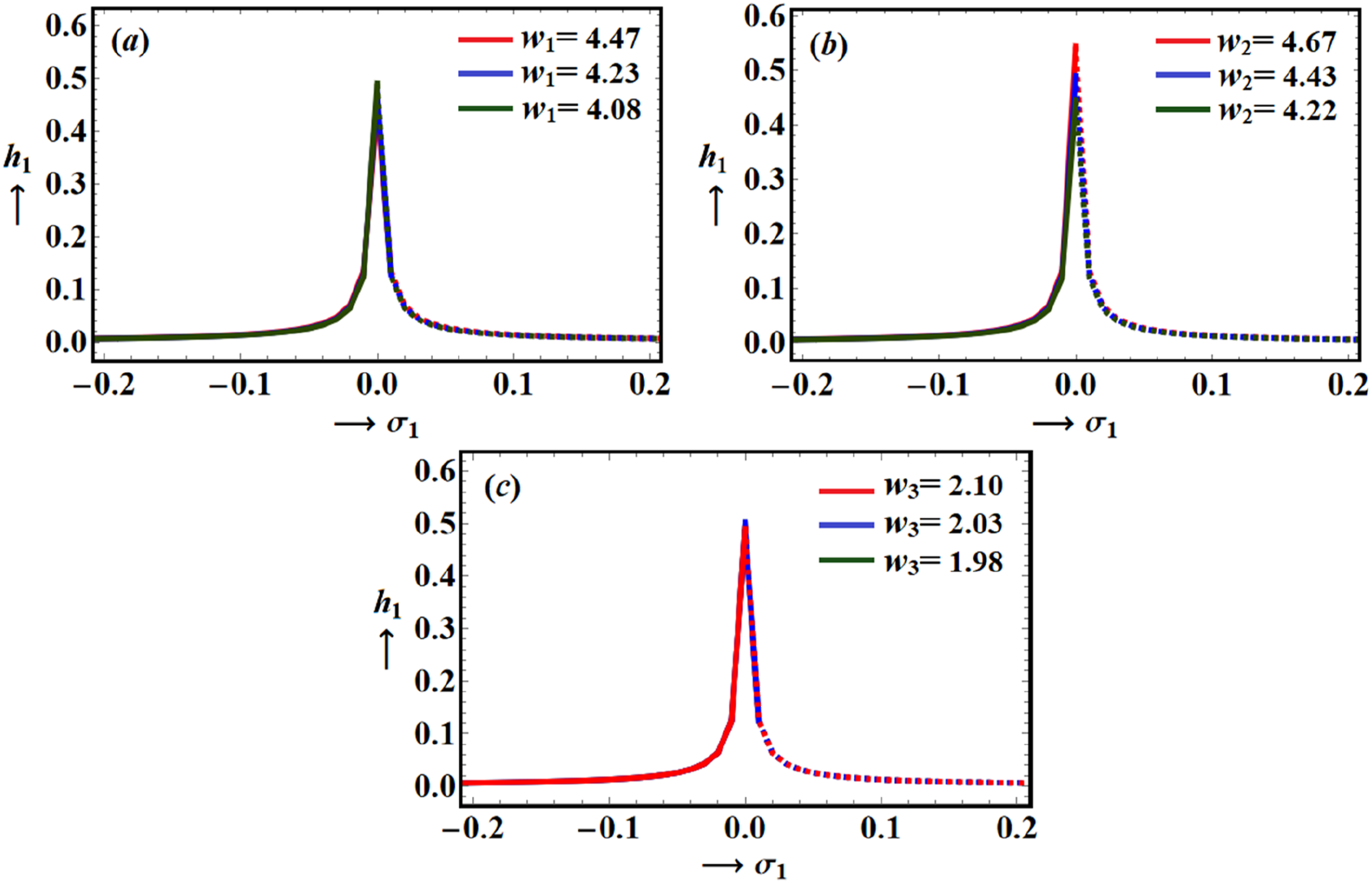
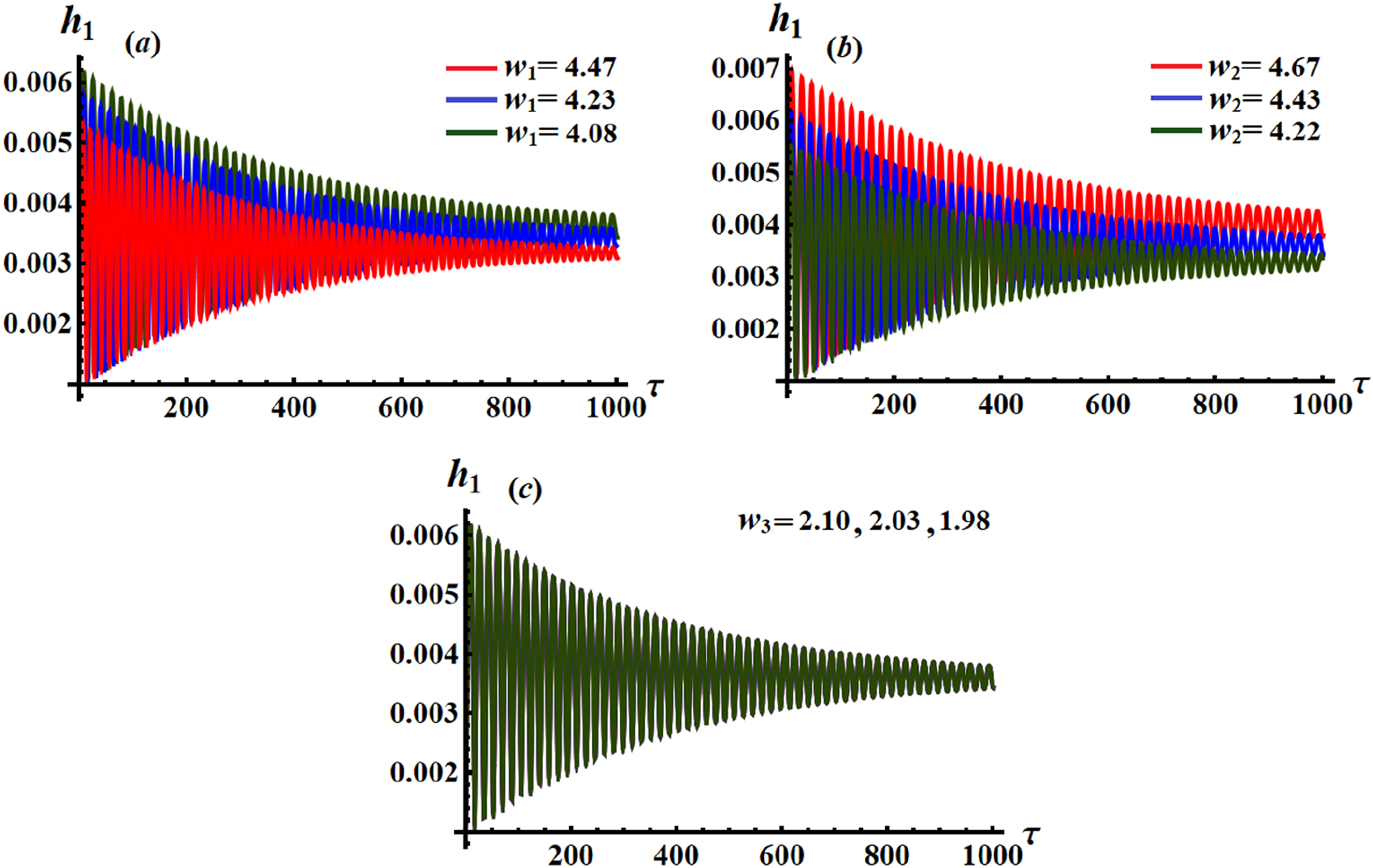
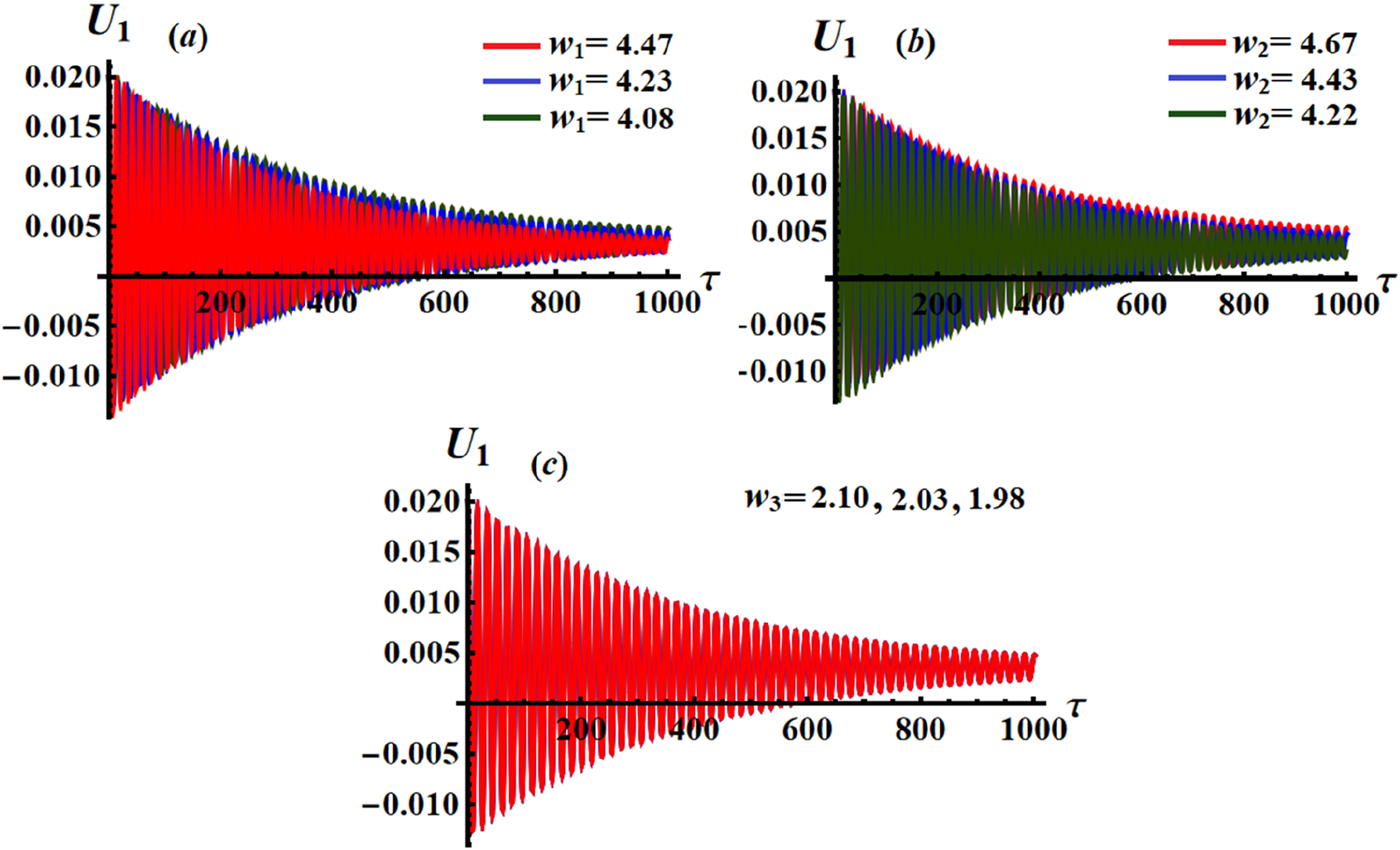
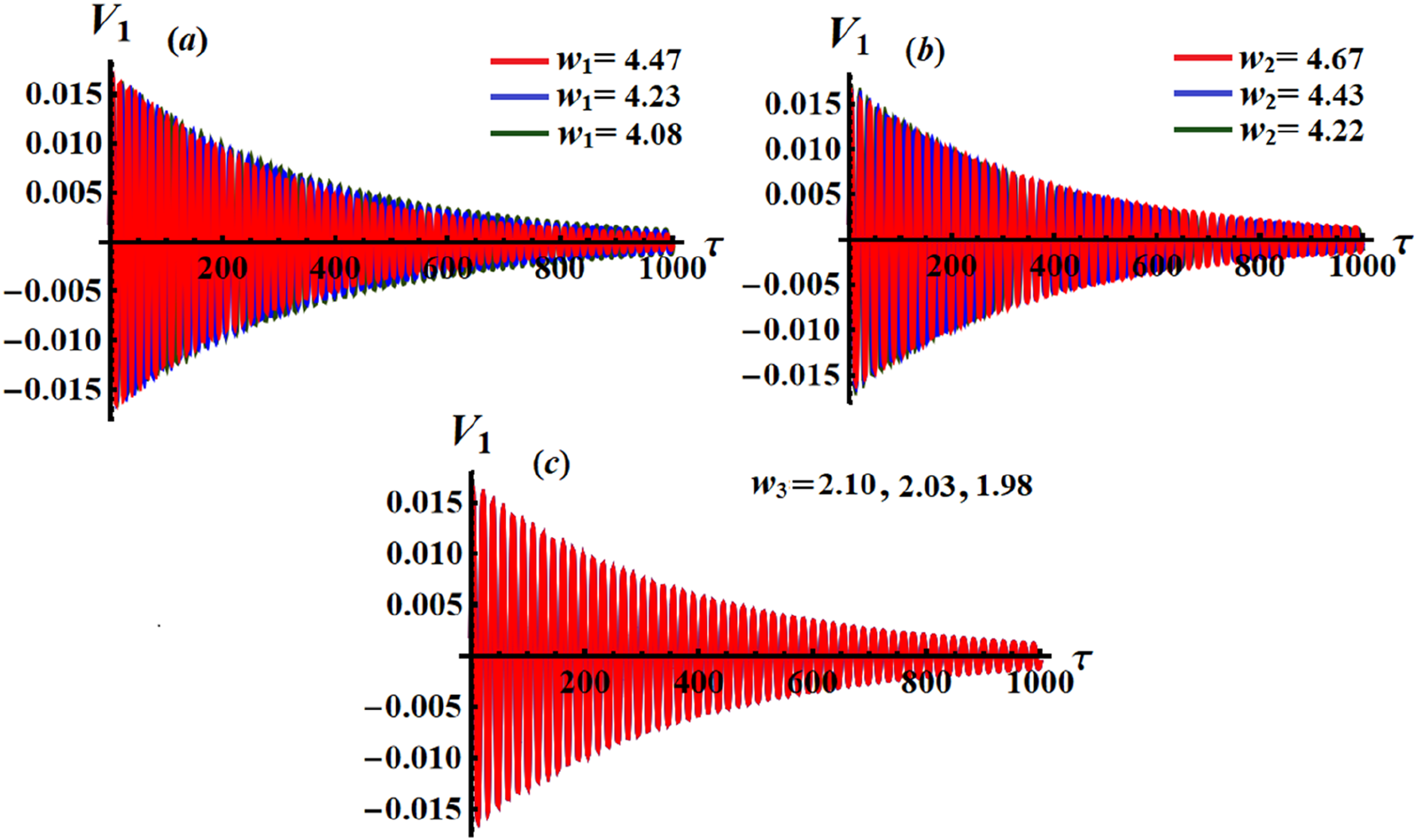
Illustrates the variation in the adjusted amplitude $h_{1}$ versus $τ$ at: (a) $w_{1} = (4.47, 4.23, 4.08) s^{‐ 1}$ , (b) $w_{2} = (4.67, 4.43, 4.22) s^{‐ 1}$ , (c) $w_{3} = (2.10, 2.03, 1.98) s^{‐ 1}$ .

Figure 3.

Reveals the time history of $h_{2}$ across different values of $w_{j} (j = 1, 2, 3)$ .

Figure 4.

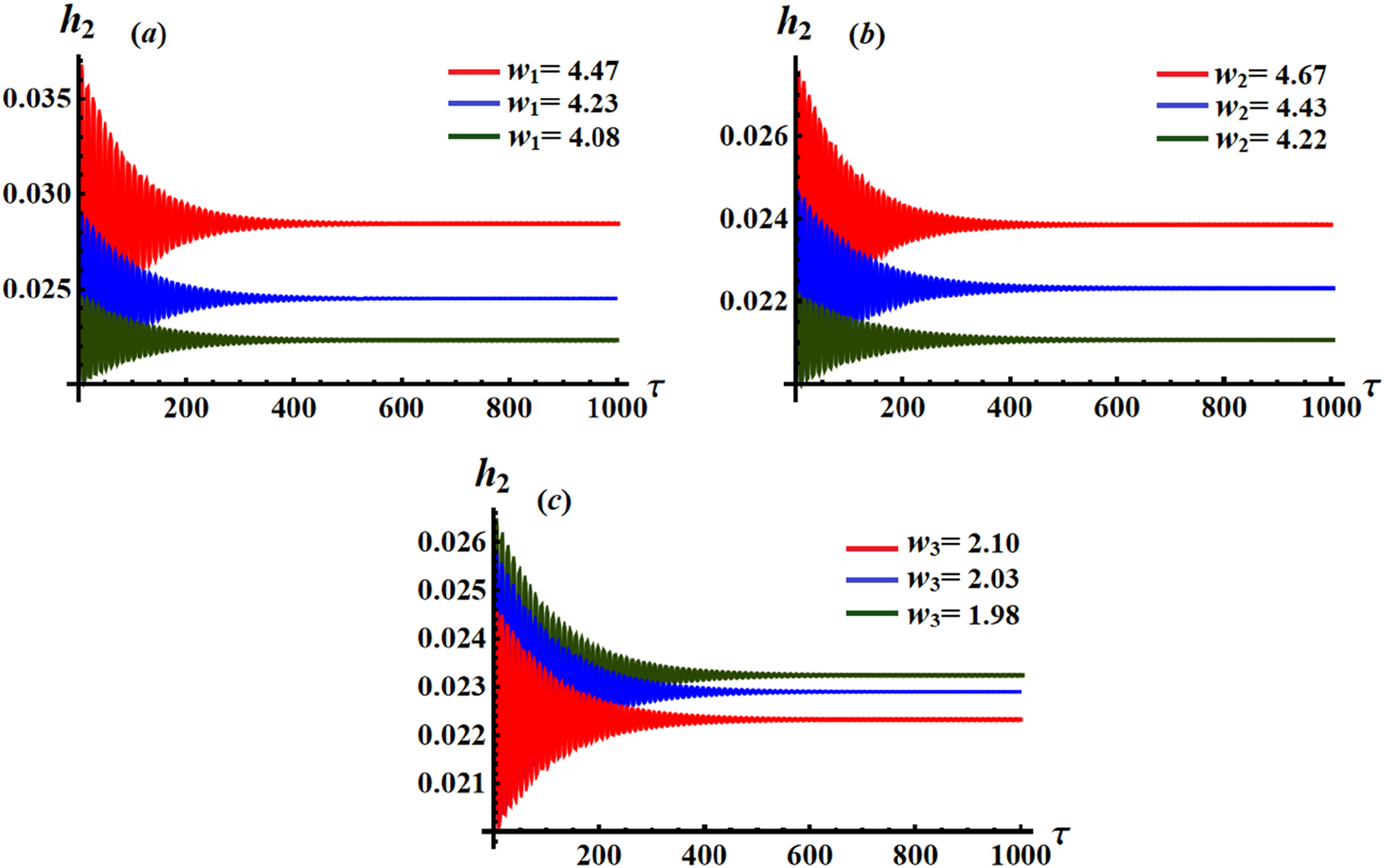
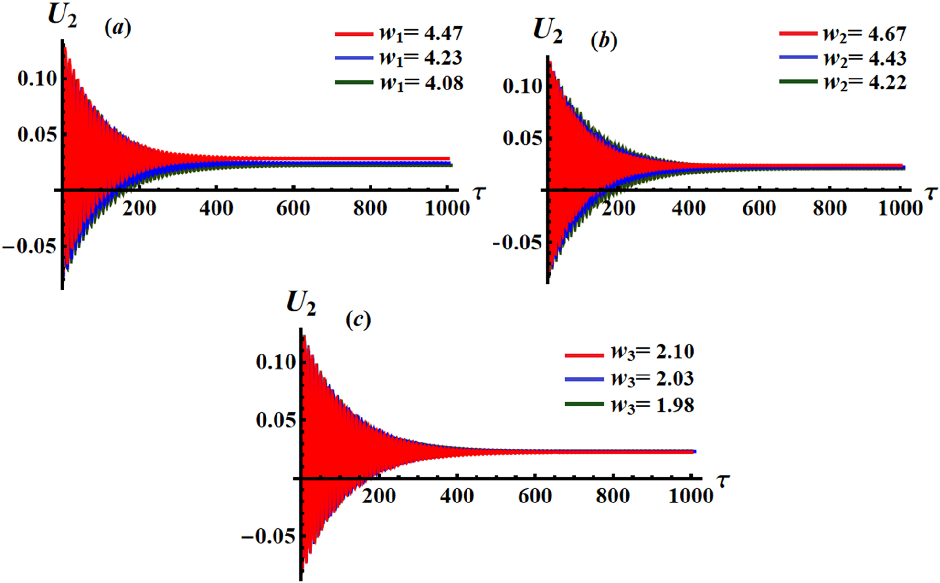
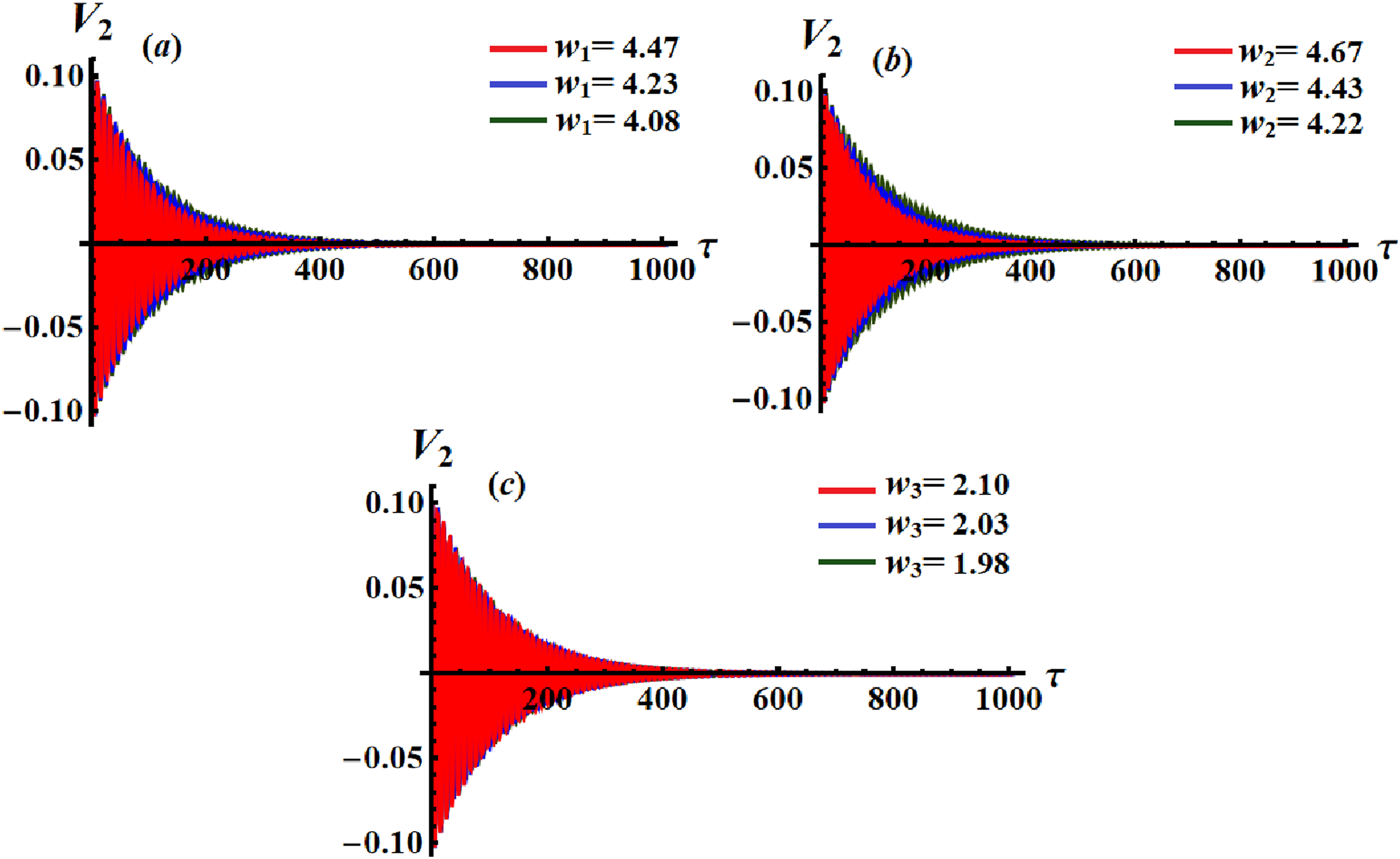
Illustrates the temporal history of $h_{3}$ at different values of $w_{j} (j = 1, 2, 3)$ .

Figure 5.

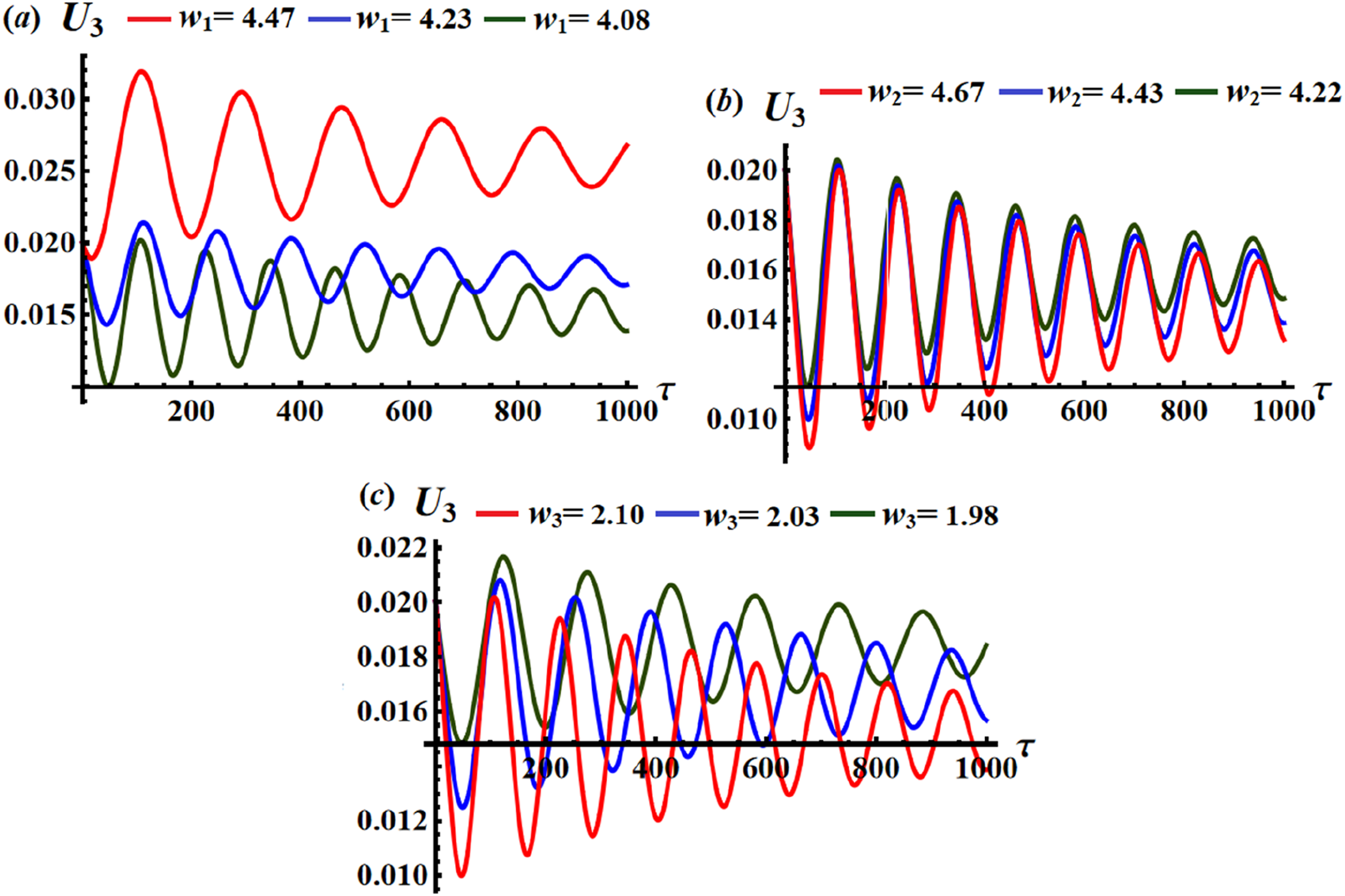
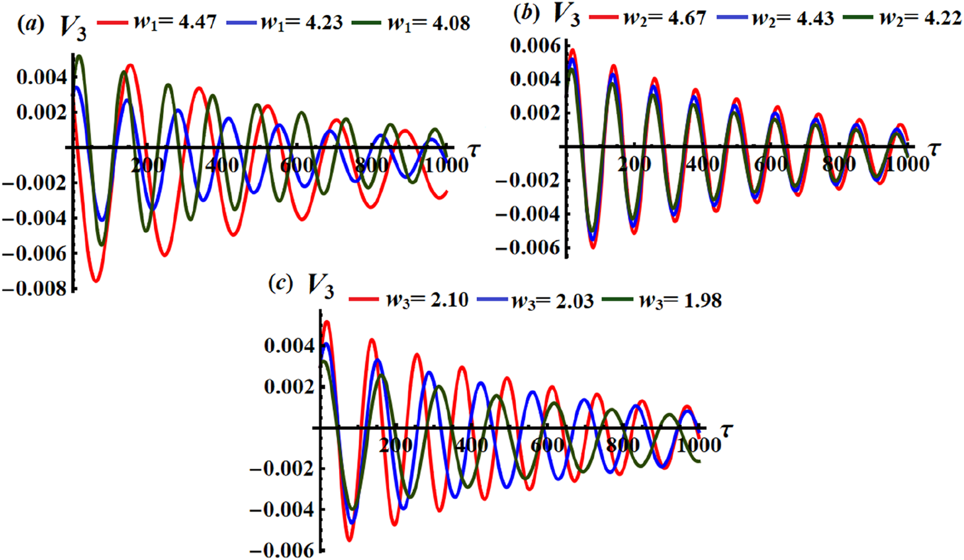
Illustrates the behavior of $θ_{1} (τ)$ at: (a) $w_{1} = (4.47, 4.23, 4.08) s^{‐ 1}$ , (b) $w_{2} = (4.67, 4.43, 4.22) s^{‐ 1}$ , (c) $w_{3} = (2.10, 2.03, 1.98) s^{‐ 1}$ .

Figure 6.

Showcases the behavior of $θ_{2} (τ)$ at various values of $w_{j} (j = 1, 2, 3)$ .

Figure 7.

Displays the behavior of $θ_{3} (τ)$ at various values of $w_{j} (j = 1, 2, 3)$ .

These figures explore the influence of system’s parameters on the time behavior of the amplitudes $h_{j} (j = 1, 2, 3)$ and modified phases $θ_{j}$ for various values of $w_{j}$ . Generally, it must be mentioned that these values are associated with the pendulum’s standard length of the arm $l$ , the rigid body mass $m$ , and the moment of inertia $U_{A}$ .

As observed from the depicted waveforms in these figures, they display diminishing patterns over time, suggesting that their behavior is stable. It is seen that $h_{1}$ has been influenced by the change of $w_{1}$ and $w_{2}$ values. The decaying manner of the waves decrease with the increase of $w_{1}$ and decrease with $w_{2}$ values, as evidenced in Figure 2(a) and (b), respectively. Conversely, $w_{3}$ values have no discernible effect on the waves’ behavior, as demonstrated in Figure 2(c). This observation aligns with the mathematical formulas governing the system of equation (60).

Parts of Figure (3) illustrate the changes in $h_{2}$ overtime as $w_{1}, w_{2},$ and $w_{3}$ undergo changes. It’s clear that an elevation in $w_{1}$ values leads to a rise in the vertical extent of the wave represented by $h_{2}$ , whereas the decay of the waves follows the direction of the minimum value of $w_{1}$ , as demonstrated in Figure 3(a). Raising $w_{2}$ values, results in an upsurge of the wave initially drawn near and adjacent to the $h_{2}$ -axis, followed by a decay in the wave until it stabilizes after the first third of the examined time period, as drawn in Figure 3(b). On the contrary, as depicted in Figure 3(c), an augmentation in $w_{3}$ values initially causes a reduction in the adjusted oscillations towards the $h_{2}$ -axis, with the waves eventually attaining stationary behavior at a minimum value of $w_{3}$ . From this analysis, it can be concluded that the variation of $h_{2}$ with time exhibits oscillations during the initial third of the time interval being studied, but eventually stabilizes towards the conclusion of the time scale.

The temporal fluctuation of the amplitude $h_{3}$ is graphically depicted in Figure (4) when considering various values of $w_{j}$ . It’s observed that the oscillations’ number in the waves describing $h_{3}$ is fewer when compared to the fluctuations in $h_{1}$ and $h_{2}$ . The primary physical rationale for these variations is attributed to the systematic construction of the equations within the system (60). In general, the decaying behavior of the depicted waves in this figure is observed throughout the entire time interval.

The following Figures (5)-(7) illustrate how the modified phases $θ_{j}$ vary over time $τ$ as the values of $w_{j}$ differ. It was observed that altering the values of $w_{j}$ has a minimal impact on the waves representing the behavior of $θ_{1}$ , as seen in Figure (5). Conversely, this effect becomes more pronounced as we move to the waves of $θ_{2}$ and $θ_{3}$ , as explored in Figures (6) and (7), respectively. Symmetric decaying curves are observed about a parallel horizontal axis to $τ$ -axis. The adjusted oscillations to the $θ_{2}$ -axis increase with the increase of $w_{1}$ and $w_{2}$ , as indicated in Figure 5(a) and (b), respectively. In a given context of the analysis of Figure 5(c) that is associated with changes in the variable $w_{3}$ , one can say that the plotted waves exhibit a decreasing trend as the values of $w_{3}$ increase. It is clear from the Figures (5) and (6) that the intensity of vibrations is greater than in Figure (7), where the reason is due to the mathematical formulas present in the system (60). The waves plotted in Figure (7) behave in a decaying manner over time. In part (a), the amplitudes of the plotted waves and their oscillations number decrease as $w_{1}$ increases, whereas in parts (b) and (c), one can observe an increasing trend in their amplitudes.

In summary, decaying waves play a crucial role in controlling vibrations, enhancing stability, improving performance, ensuring safety, and reducing noise in vibrating systems.

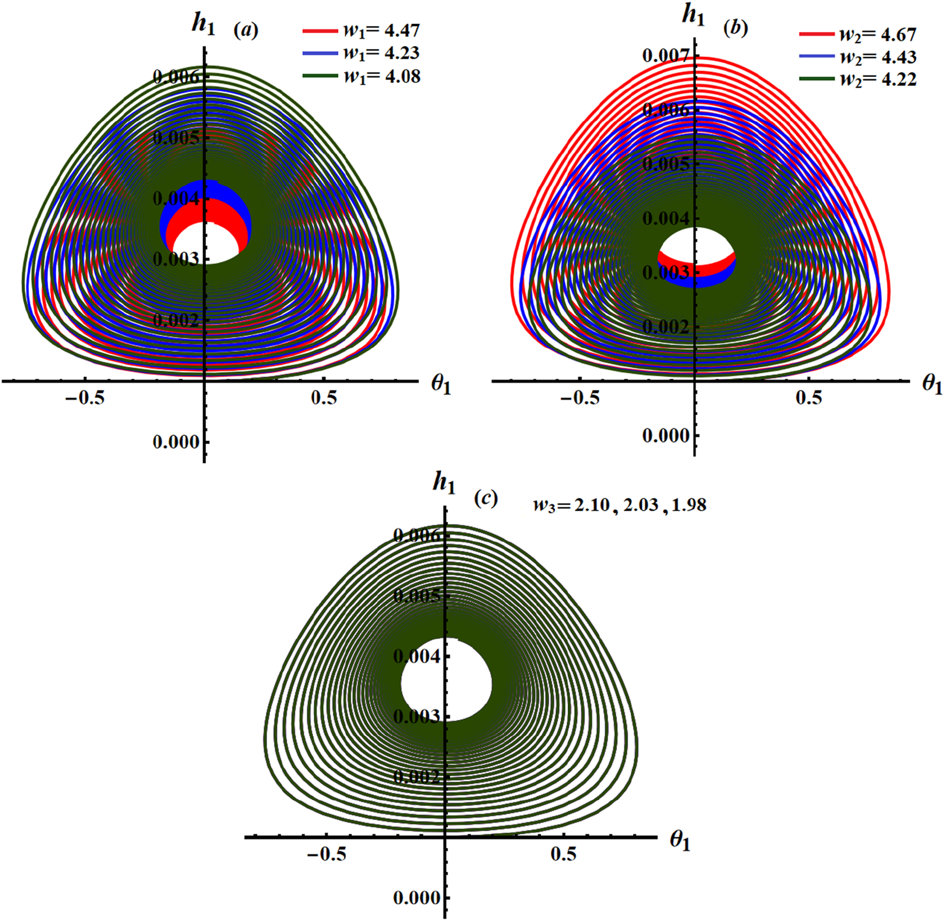
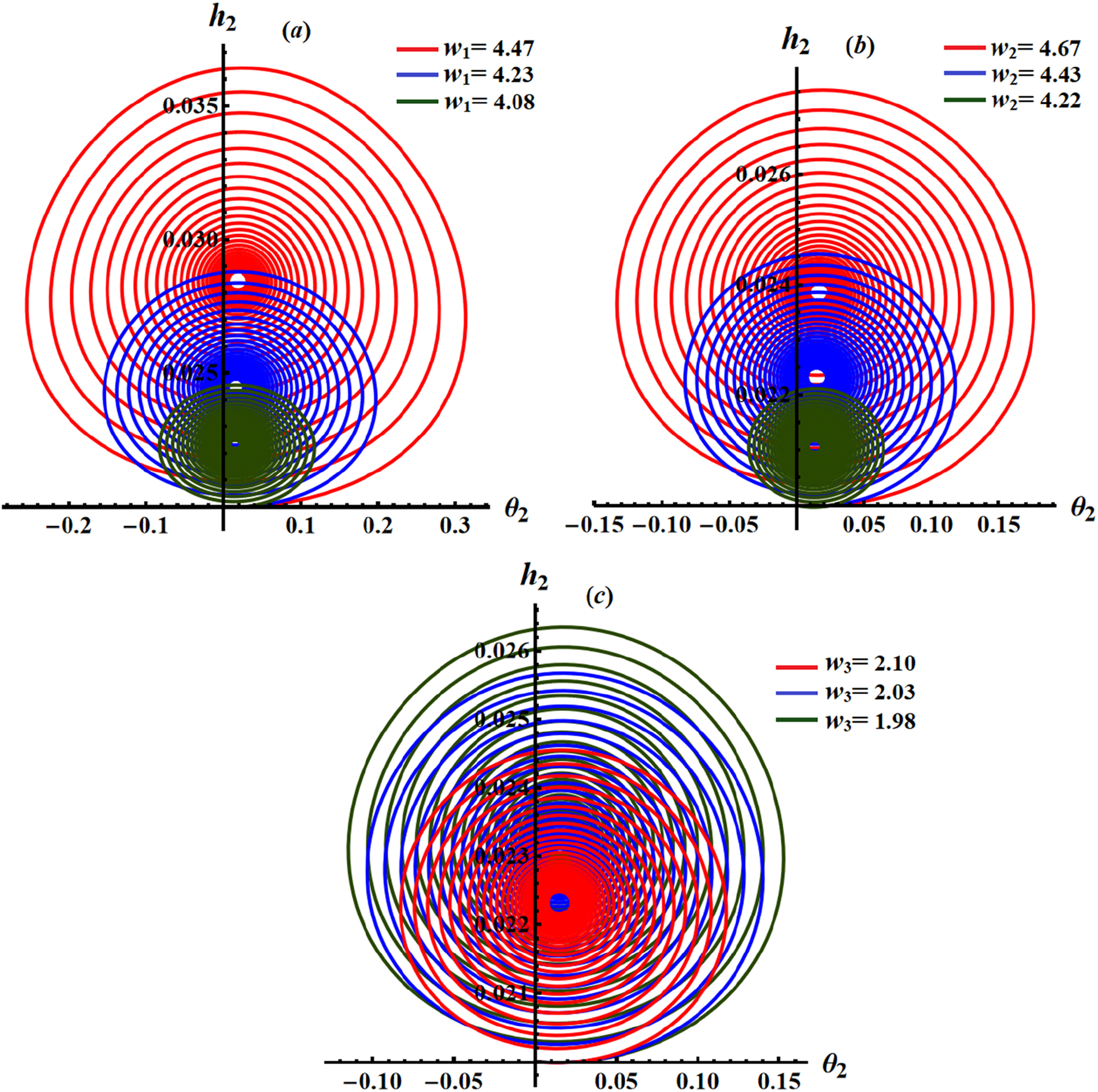
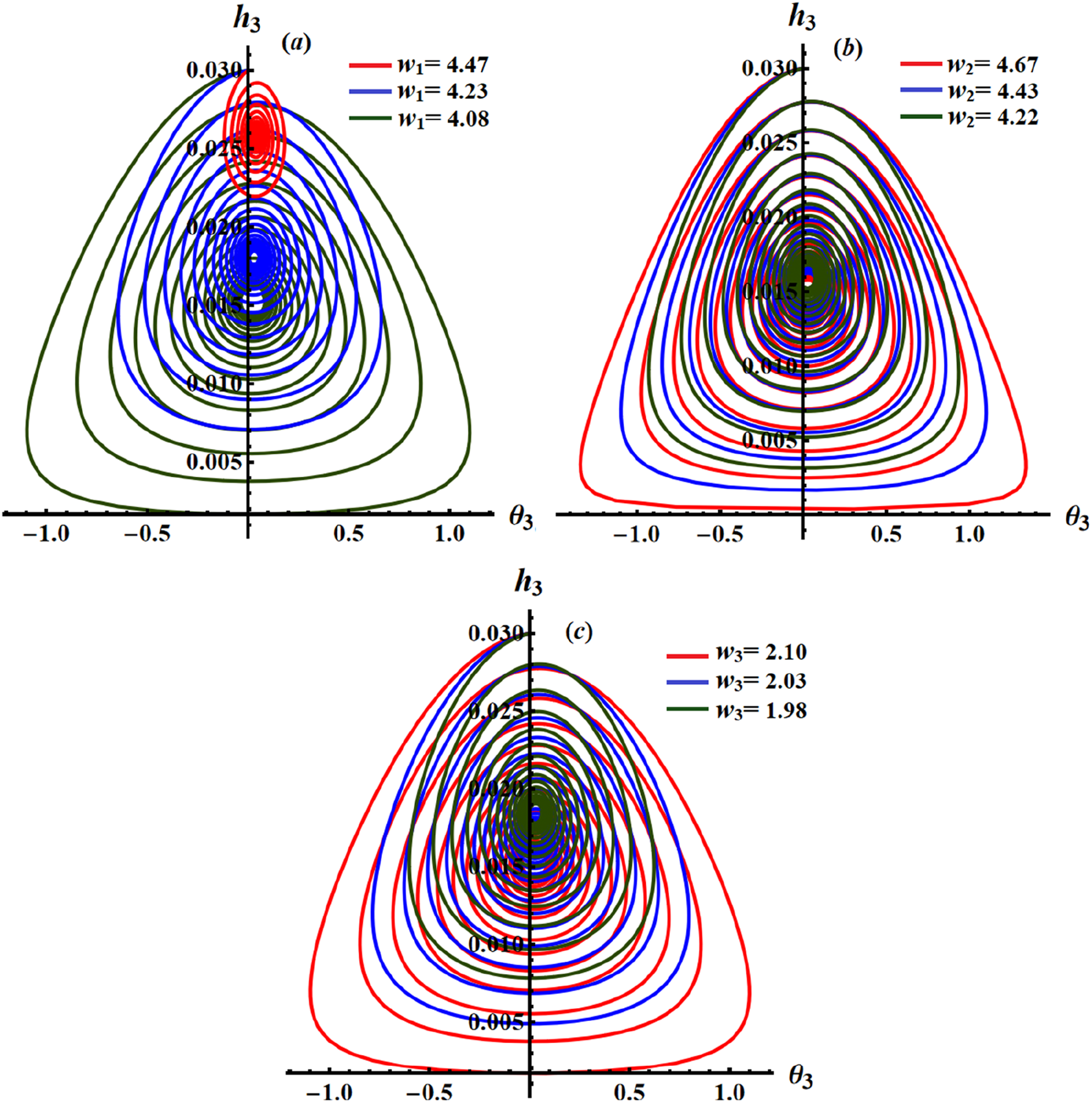
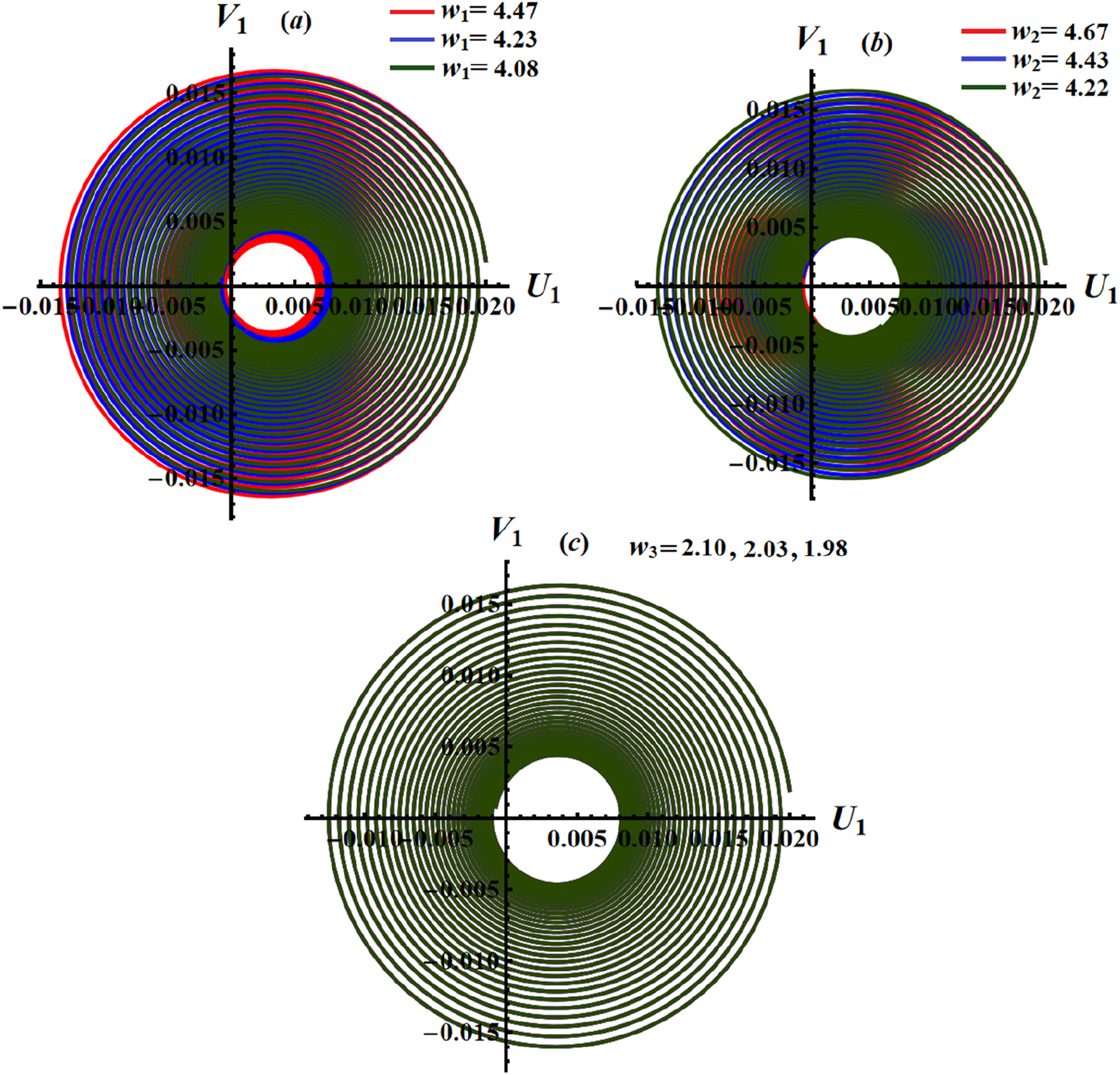
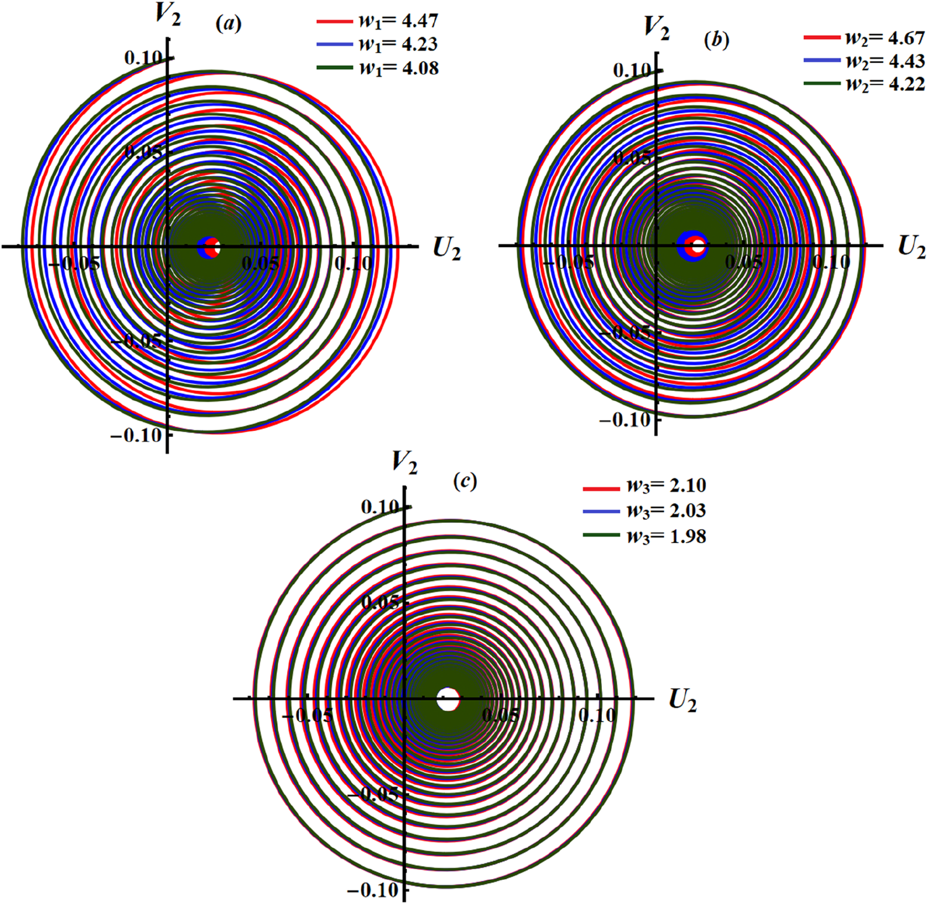
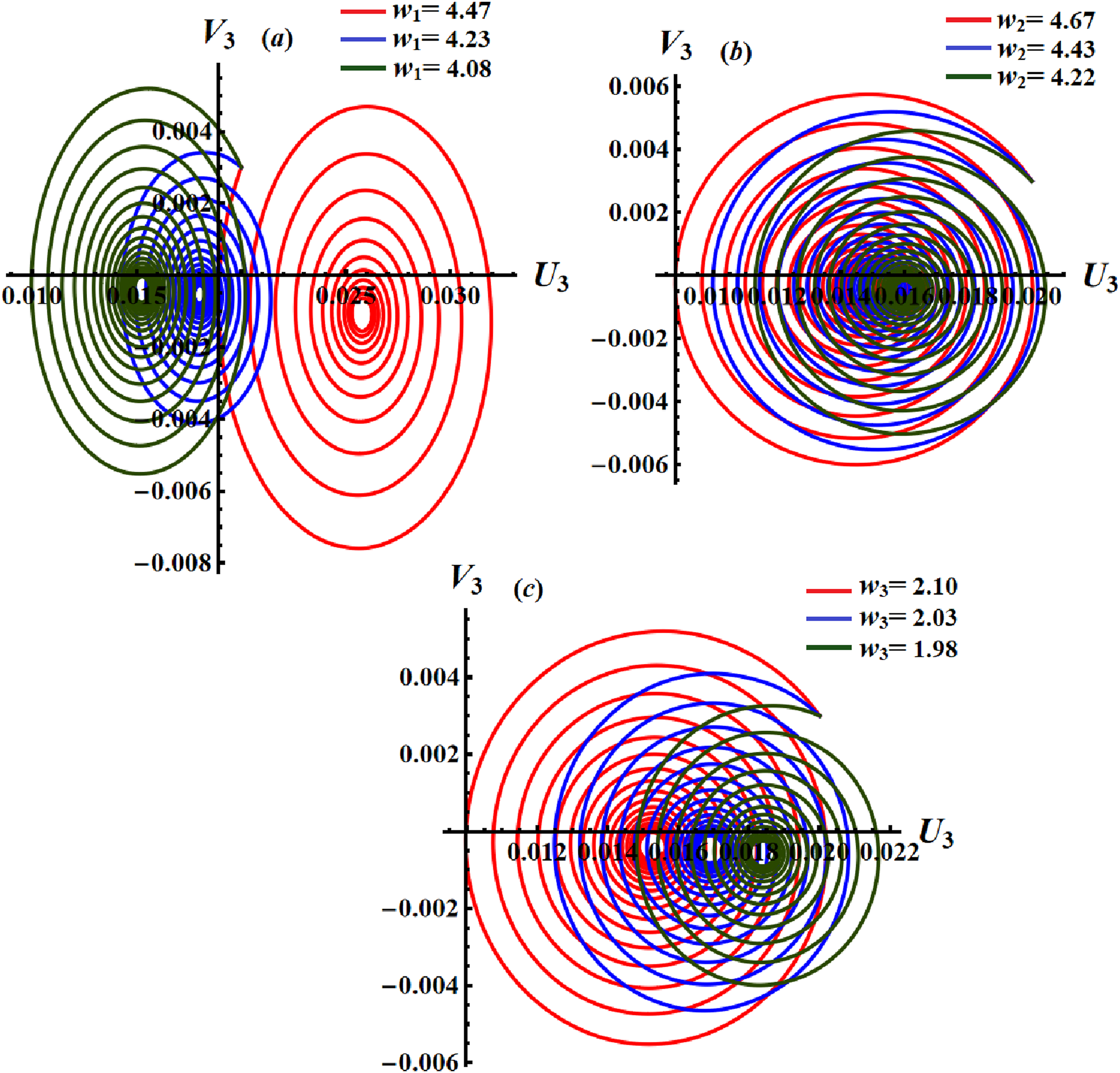
It’s notable that the patterns exhibited by the curves in Figures (2)-(7) can be interpreted graphically between adjusted amplitudes and phases. This can be done when the temporal parameter is excluded from the relationships that govern them, resulting in spiral curves, as seen in Figures (8)-(10). Each curve converges towards a single point in the planes $h_{j} θ_{j}$ , when $w_{j}$ vary affirming the inherent stability of these waves. Overall, spiral plane curves provide valuable insights into the behavior of vibrating systems, aiding in stability analysis, mode shape representation, frequency response (FR) visualization, and damping analysis.

Figure 8.

Describes the curves in the $θ_{1} h_{1}$ plane at different values of $w_{j} (j = 1, 2, 3)$ .

Figure 9.

Illustrates the curves in the $θ_{2} h_{2}$ plane at distinct values of $w_{j} (j = 1, 2, 3)$ .

Figure 10.

Illustrates the phase curves in $θ_{3} h_{3}$ plane for different values of $w_{j} (j = 1, 2, 3)$ .

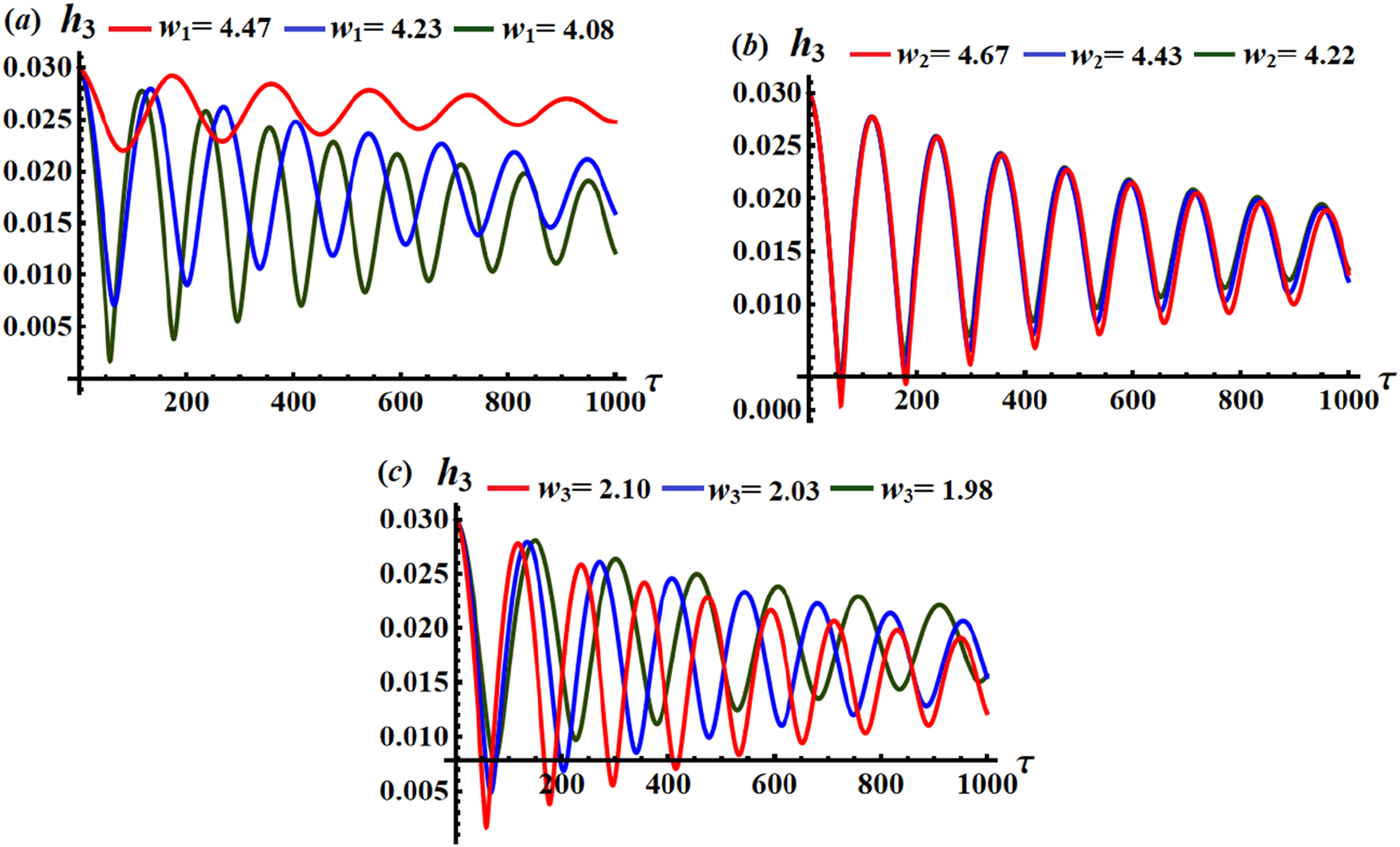
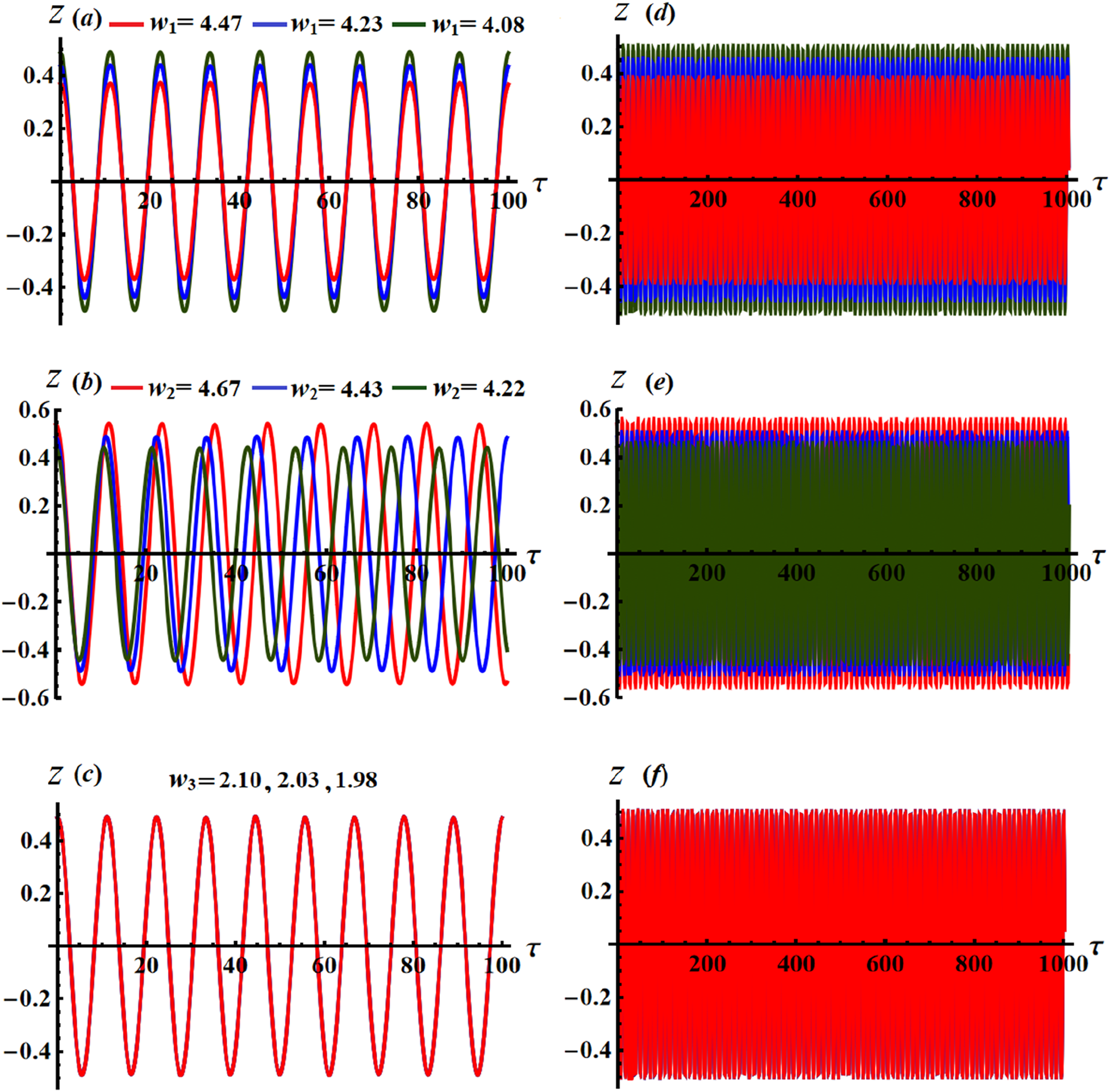
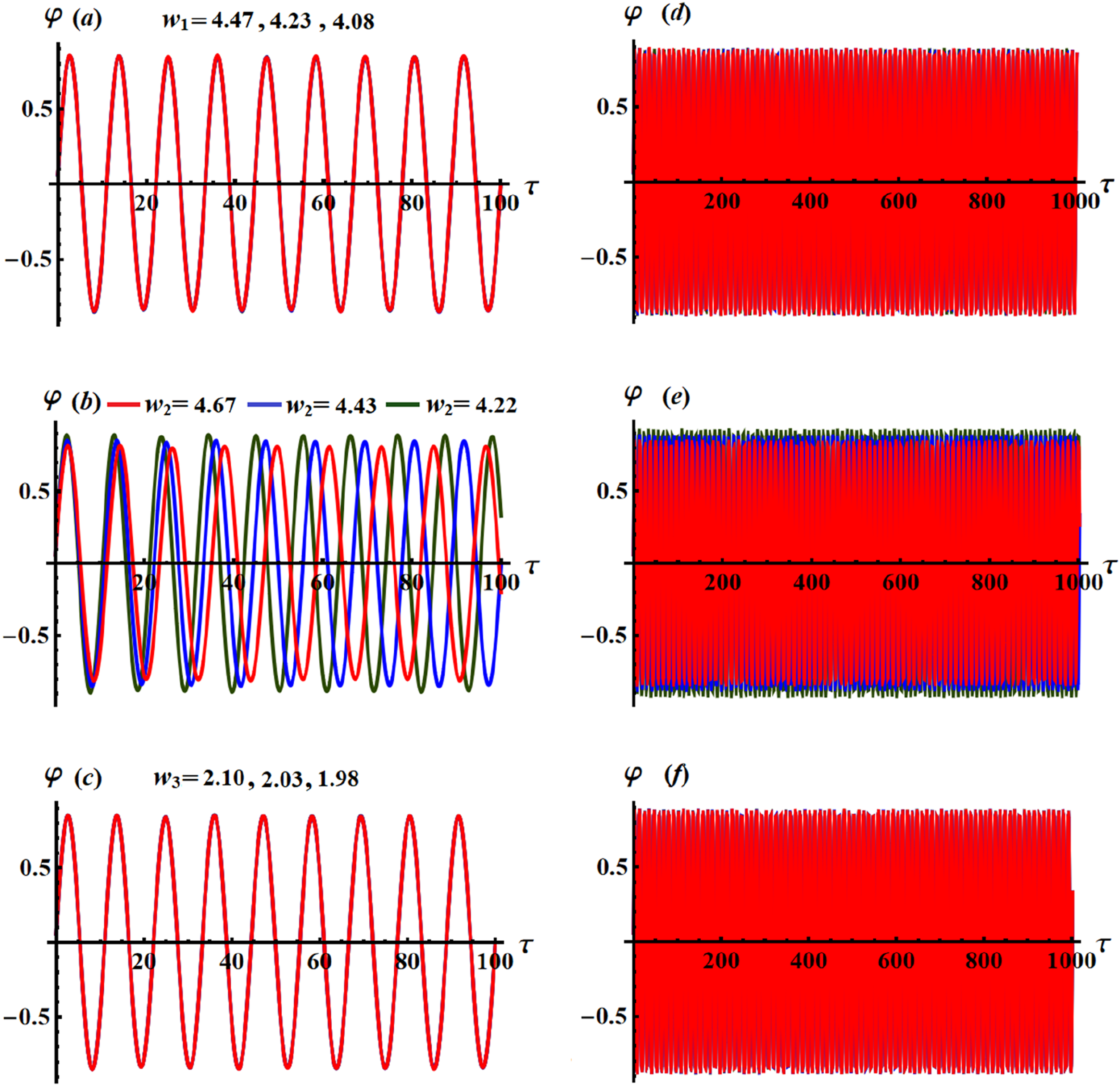
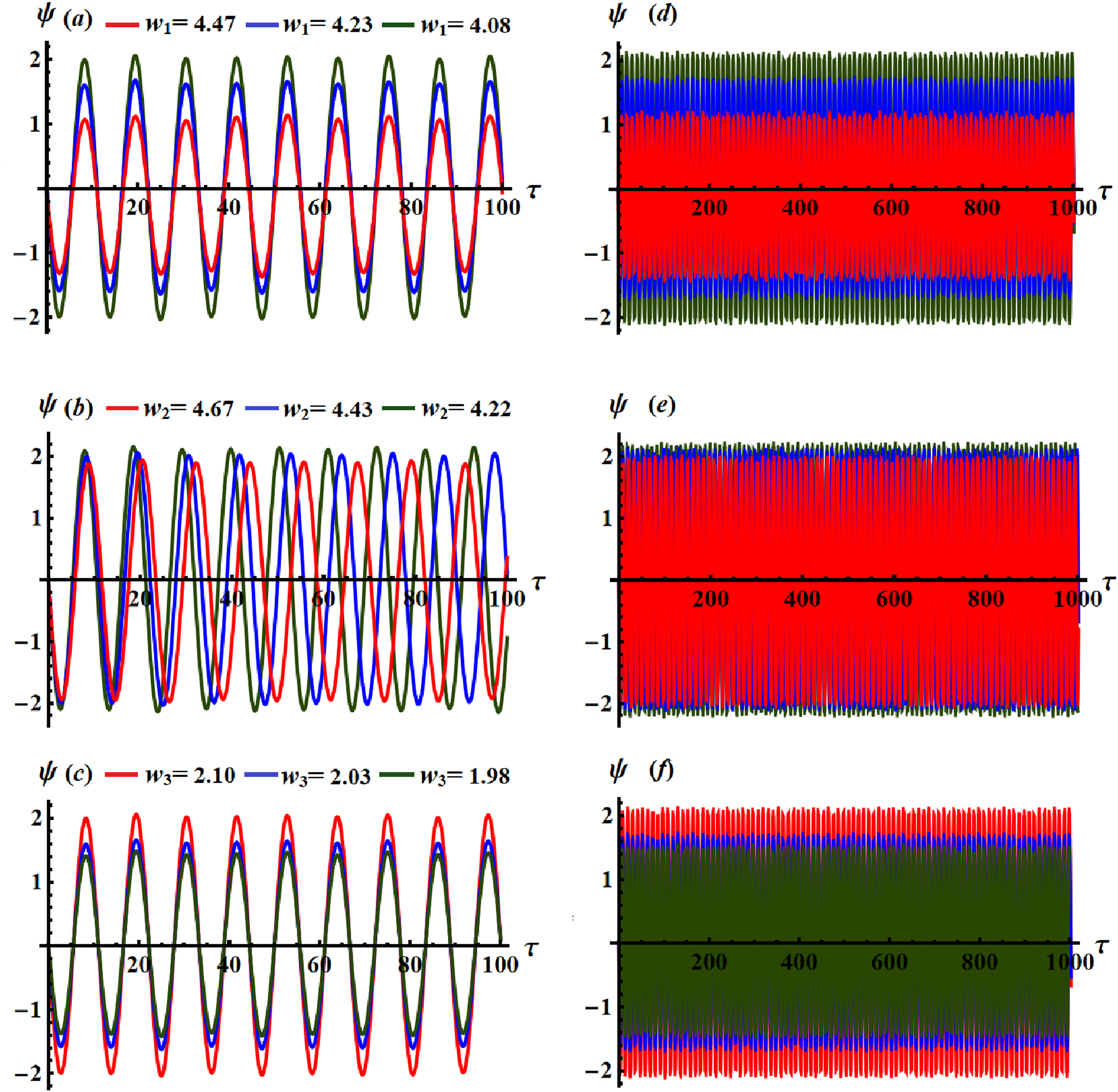
The curves depicted in Figures (11)-(13) illustrate the temporal evolution of solutions $z, φ,$ and $ψ$ across distinct time intervals, two different time ranges, highlighting the overarching shape of the outcomes. The plotted curves exhibit periodic wave patterns, signifying the stability of the obtained solutions. A detailed examination of Figure (11) reveals that the plotted waves in segments (a) and (d ) manifest as standing waves with discernible nodes. Notably, their amplitudes escalate alongside the increase in $w_{1}$ values, while maintaining a consistent number of oscillations and wavelengths. Figure 11(b) and (e) present progressive waves evolving over time in response to varying $w_{2}$ values, where their amplitudes diminish proportionally with the growth of these values. The periodic waves in segments (c) and ( f ) exhibit no alteration with the augmentation of $w_{3}$ .

Figure 11.

Showcases the efficiency of $w_{j} (j = 1, 2, 3)$ values on the solution $z$ .

Figure 12.

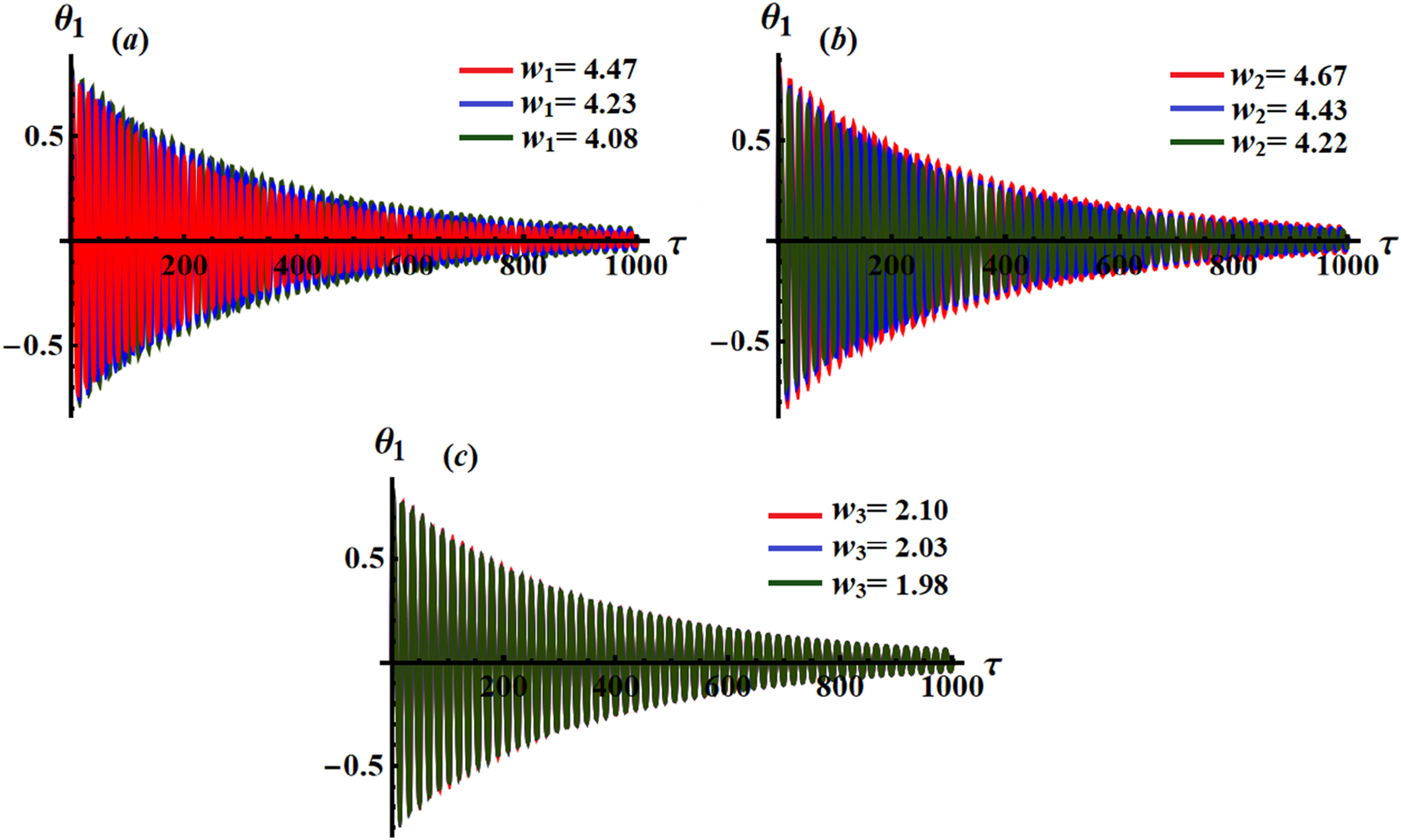
Demonstrates the impact of $w_{j} (j = 1, 2, 3)$ values on the solution $φ$ .

Figure 13.

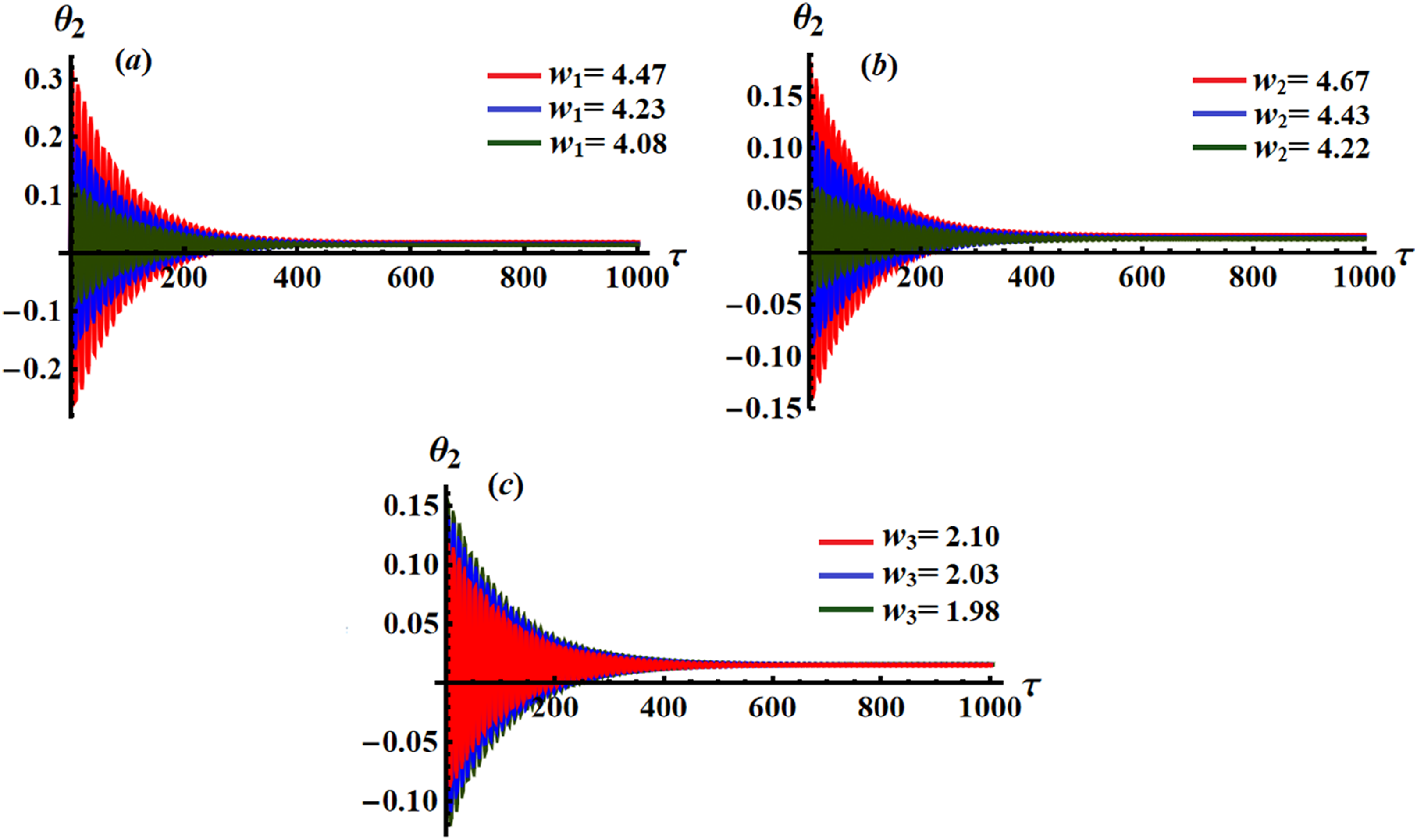
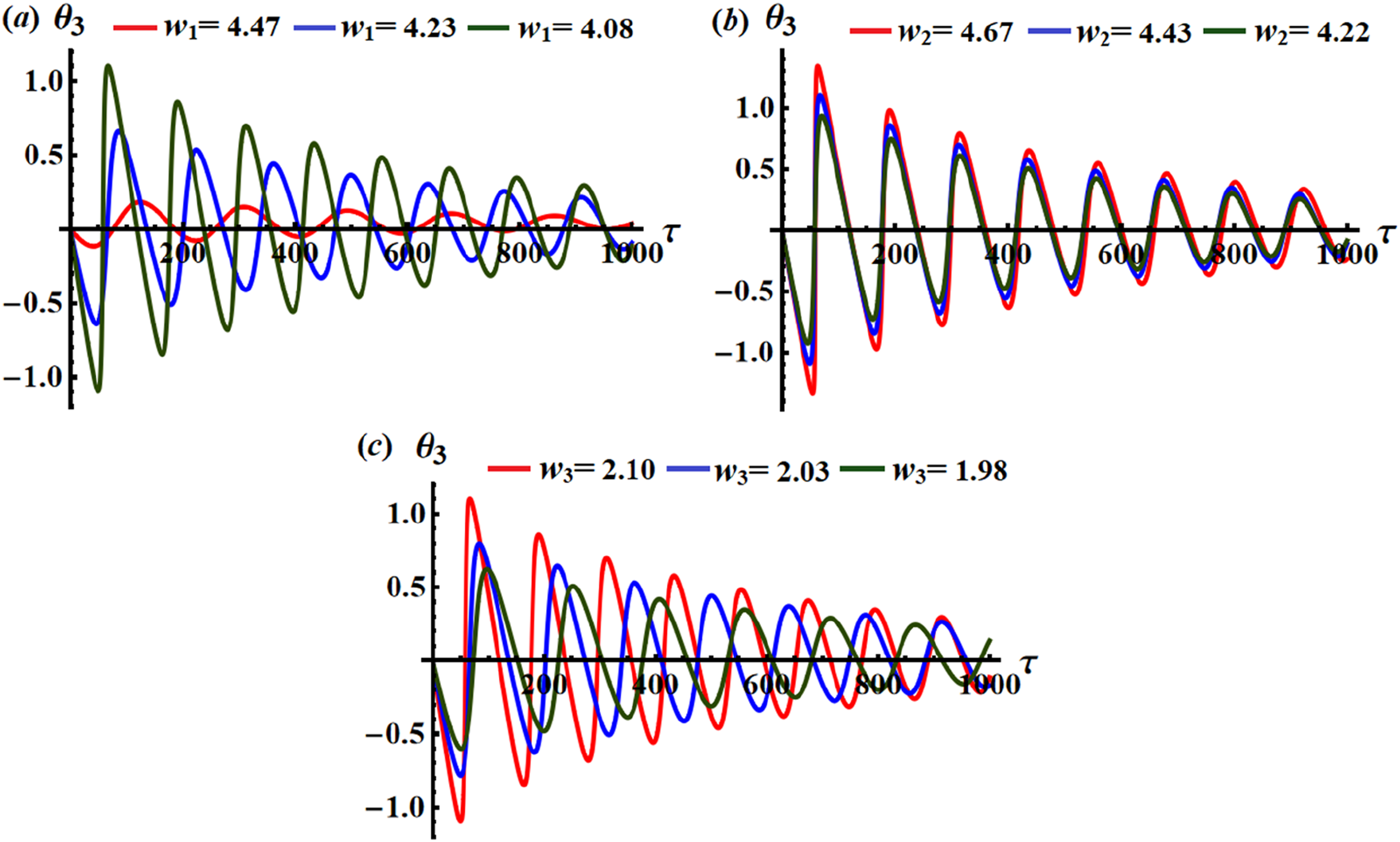
Shows the impact of changes in $w_{j} (j = 1, 2, 3)$ on the solution $ψ$ .

A closer examination of the presented waves in Figure 12(a), (d) and (c), (f) shows that the solution $φ$ does not vary with the change in $w_{1}$ and $w_{3}$ values, while it has been varied with the variation of $w_{2}$ values, as seen in Figure 12(b) and (e). The rationale behind this lies in the mathematical structure of this solution, where it explicitly depends on $w_{2}$ .

An examination of the graphed waves in Figure (13) shows that how the solution $ψ$ fluctuates in response to changes in $w_{j}$ values. As the mathematical structure of this solution explicitly relies on $w_{j}$ values, it’s reasonable to anticipate that it will be influenced by variations in $w_{j}$ values. Curves of this figure affirm this prediction, showcasing standing waves with discernible nodes are observed in Figure 13(a), (d)) and (c), (f), while progressive waves are noted in segments (b) and (e).

Generally, periodic waves serve as valuable indicators of stability in vibrating dynamical systems, reflecting the delicate balance between forces, resonance phenomena, damping effects, and control strategies. Analyzing the characteristics of these waves provides valuable insights into the behavior and performance of complex systems across various domains.

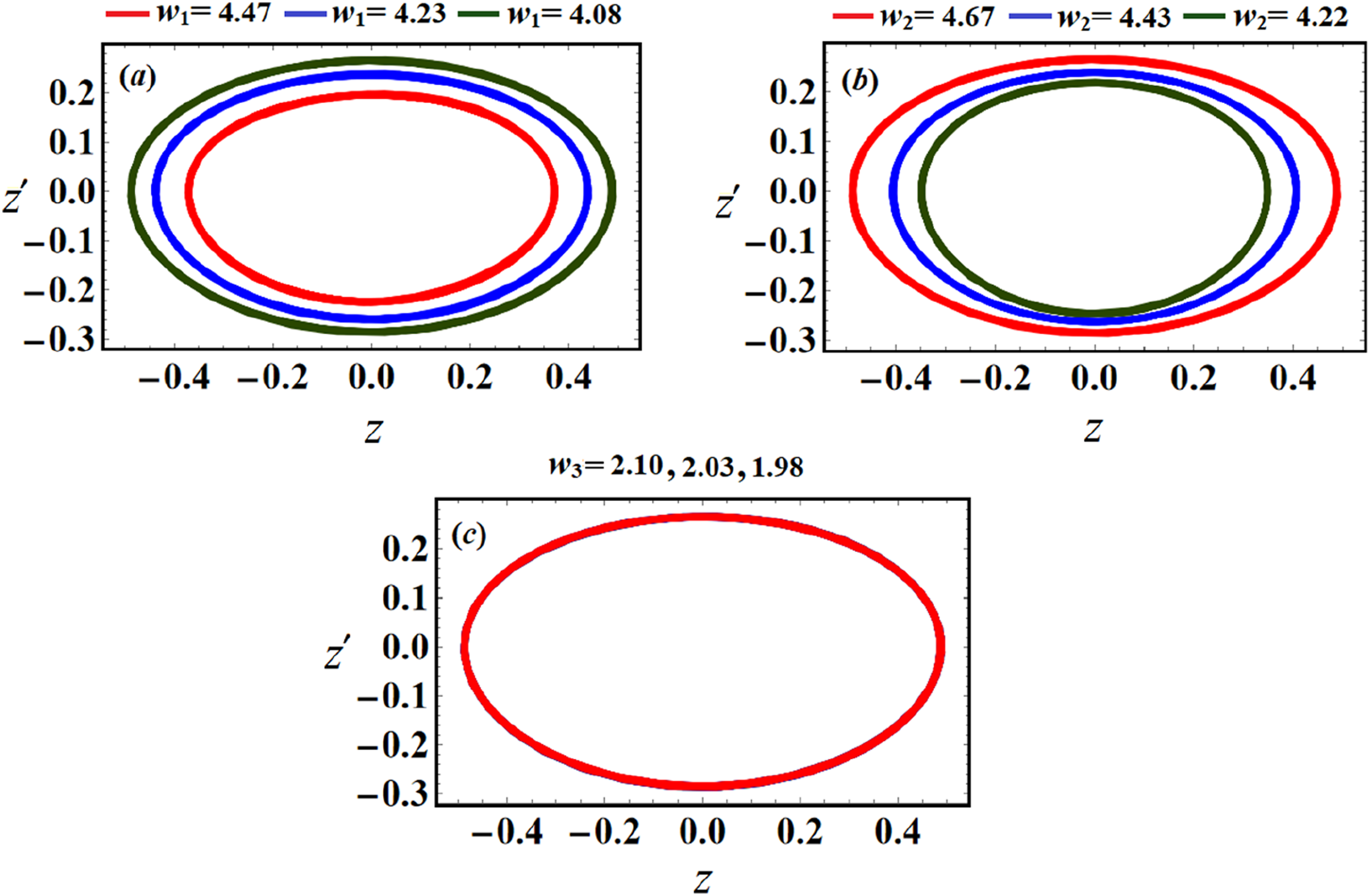
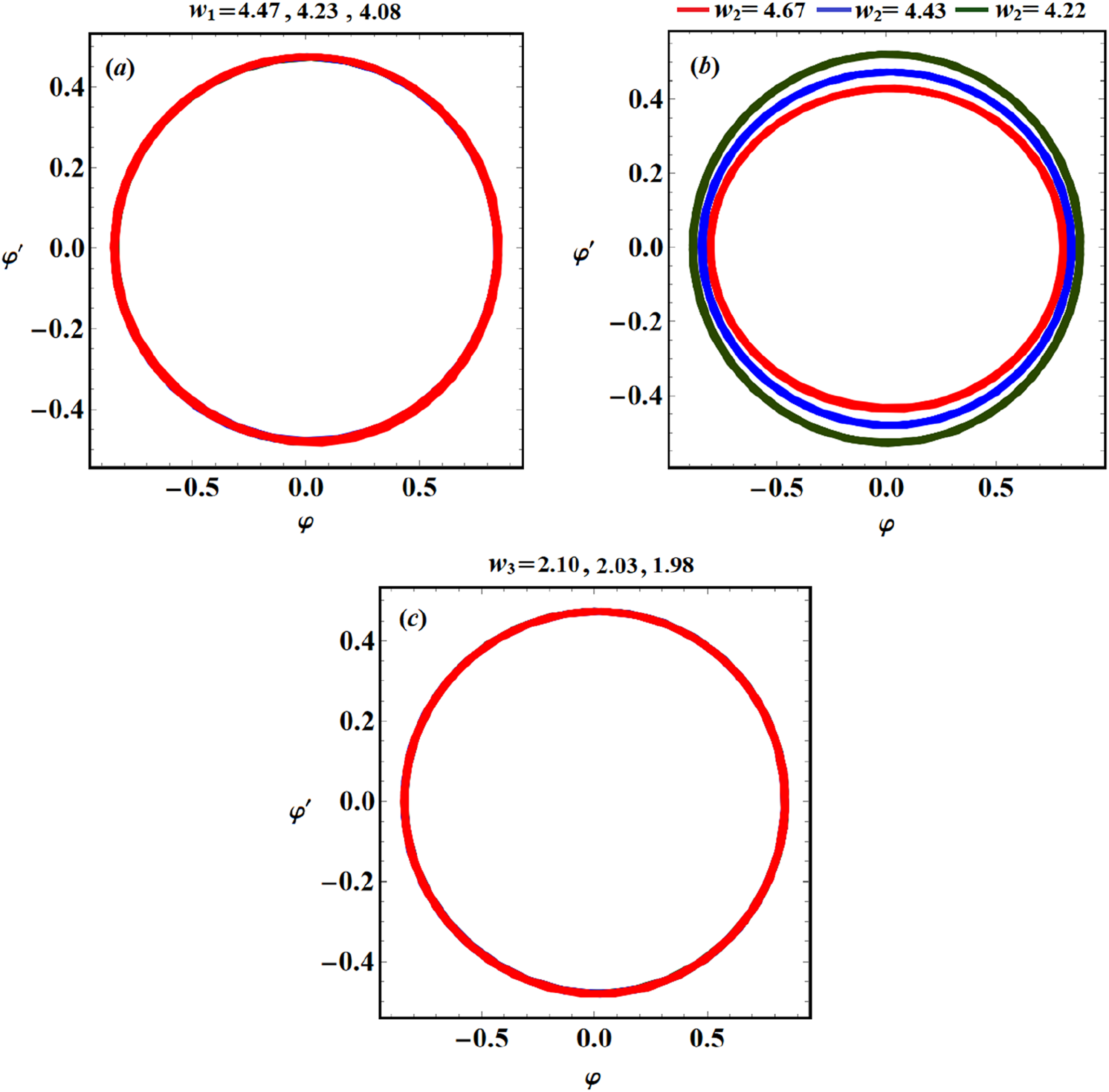
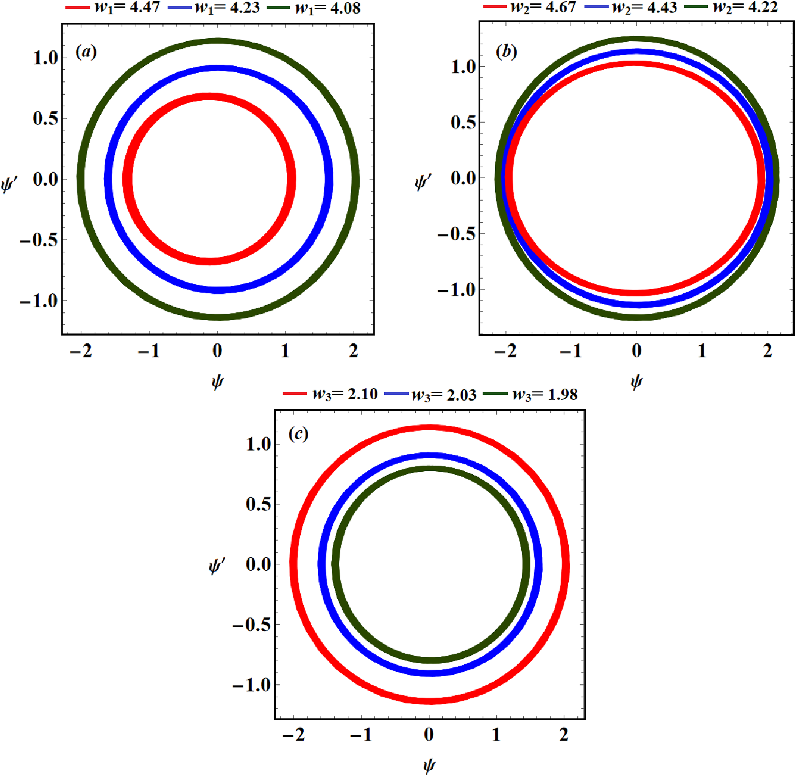
The phase plane curves corresponding to the achieved solutions are plotted in $z z^{'}, φ φ^{'},$ and $ψ ψ^{'}$ planes as, depicted in Figures (14)-(16), with variations in $w_{1}, w_{2},$ and $w_{3}$ . These curves take the form of closed loops, reinforcing the graphed curves of the aforementioned solutions and indicating their stability.

Figure 14.

The phase plane portrait of the solution $z$ at varies values of $w_{j} (j = 1, 2, 3)$ .

Figure 15.

Explores the curves in the $φ φ^{'}$ plane at various values of $w_{j} (j = 1, 2, 3)$ .

Figure 16.

Showcases the visual representations of the curves in $ψ ψ^{'} \to$ plane at the aforementioned values of $w_{j} (j = 1, 2, 3)$ .

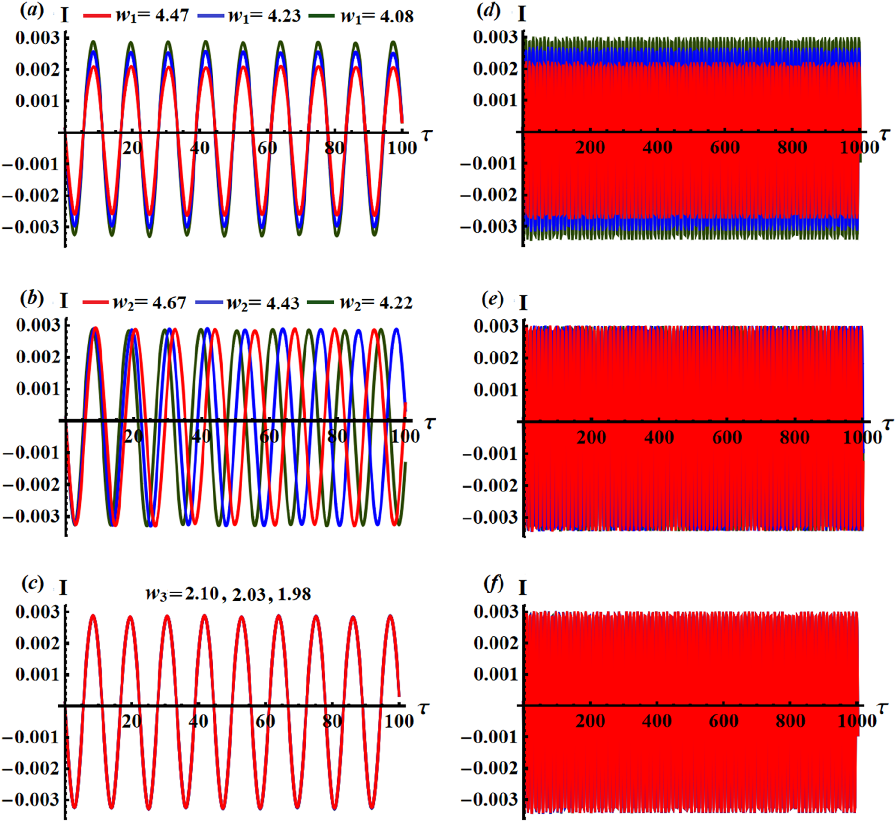
The periodic waves in Figures (17) and (18) illustrate the variation of the generated current $I$ and power $P$ at various values of $w_{j}$ during short and large scales of time. Minimal amplitudes of the current generated by the harvesting circuit is demonstrated, leading to low-power levels at the output within the milliwatts range, which is ideal for certain applications. The current exhibits a positive correlation with the change in $w_{1}$ and $w_{2}$ values, as evidenced by the presence of standing and progressive waves observed in Figure 17(a), (d) and (b), (e). On the contrary, the current $I$ shows no variation with the change in $w_{3}$ values, as noted in segments (c) and (e) of this figure.

Figure 17.

Identifies the chronological progression of the generated current $I$ at various values of $w_{j} (j = 1, 2, 3)$ .

Figure 18.

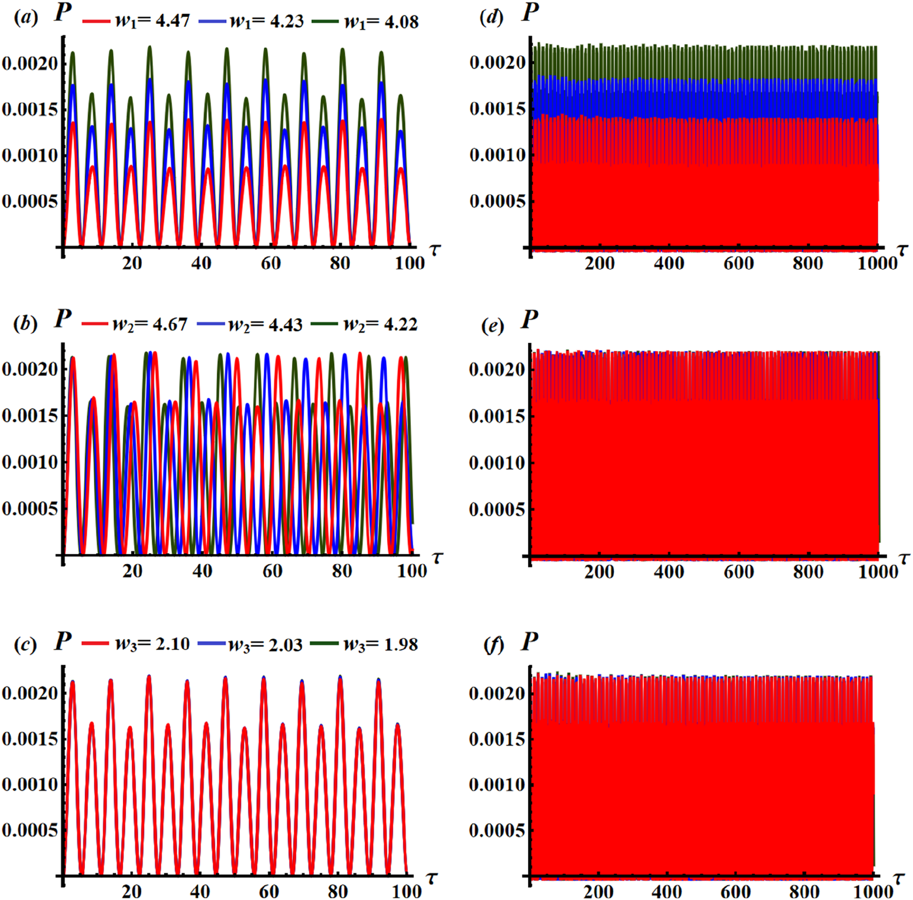
Illustrates the influences of $w_{j} (j = 1, 2, 3)$ on the output power $P$ .

Observing the depicted waves in Figure (18), it’s apparent that the generated power $P$ exhibits periodic behavior, influenced by variations in both $w_{1}$ and $w_{2}$ values, with slight alterations noted in response to changes in $w_{3}$ values.

In the systems energy harvesting, the power output depends on both the current generated by the harvesting device and the voltage at which that current is produced. The relationship between current and power varies depending on the specific characteristics of the energy source, the efficiency of the harvesting technology, and the load connected to the system. Maximizing power output typically involves optimizing the harvesting device’s design and operating conditions to achieve the desired balance between current and voltage.

Solutions at the steady-state

This section addresses the oscillations of the mentioned model when it reaches a steady-state scenario. This means that the transient process of the oscillations disappears due to the system’s damping. In this scenario, equation (60) plays a crucial role in determining the steady-state conditions, where the amplitudes $h_{j} (j = 1, 2, 3)$ and modified phases $θ_{j}$ have zero derivatives.^50,51 Subsequently, we were able to write

\frac{d h_{j}}{d t} = \frac{d θ_{j}}{d t} = 0 .

(61)

In accordance with these conditions, the below equations are produced

f_{1} \sin θ_{1} - ω_{1} h_{1} [c_{1} + \frac{α γ}{(α^{2} + ω_{1}^{2})}] = 0,

f_{1} \cos θ_{1} + h_{1} [2 ω_{1} σ_{1} - \frac{γ ω_{1}^{2}}{(α^{2} + ω_{1}^{2})} - \frac{3 (ω_{1}^{2} - 1)}{2 (ω_{1}^{2} - 4)} h_{2}^{2}] = 0,

f_{2} \sin θ_{2} - c_{2} h_{2} = 0,

f_{2} \cos θ_{2} + h_{2} [2 σ_{2} + \frac{s}{(1 - ω_{2}^{2})} - \frac{3 (ω_{1}^{2} - 1)}{2 (ω_{1}^{2} - 4)} h_{1}^{2} + \frac{(ω_{1}^{4} + 7 ω_{1}^{2} - 8)}{8 ω_{1}^{2} (ω_{1}^{2} - 4)} h_{2}^{2}] = 0,

f_{3} \sin θ_{3} - \frac{c_{3} h_{3}}{ω_{2}} = 0,

f_{3} \cos θ_{3} + h_{3} [2 ω_{2} σ_{3} + \frac{s}{(ω_{2}^{2} - 1)} + \frac{1}{8} h_{3}^{2} - \frac{(1 - 2 ω_{2}^{2})}{4 {(1 - ω_{2}^{2})}^{2}} h_{2}^{2} + \frac{ω_{1}^{4}}{2 (4 - ω_{1}^{2} ω_{2}^{2})} h_{1}^{2}] = 0 .

(62)

It is noteworthy that the earlier system consists of six algebraic equations involving the variables $h_{j}$ and $θ_{j}$ . Upon eliminating $θ_{j}$ , we directly obtain three equations relating the amplitudes $h_{j}$ and the detuning parameters $σ_{j}$

f_{1}^{2} = 4 ω_{1}^{2} h_{1}^{2} {{[\frac{c_{1}}{2} + \frac{α γ}{2 (α^{2} + ω_{1}^{2})}]}^{2} + {[σ_{1} - \frac{γ ω_{1}}{2 (α^{2} + ω_{1}^{2})} - \frac{3 (ω_{1}^{2} - 1)}{4 ω_{1} (ω_{1}^{2} - 4)} h_{2}^{2}]}^{2}},

f_{2}^{2} = h_{2}^{2} {c_{2}^{2} + 4 {[σ_{2} + \frac{s}{2 (1 - ω_{2}^{2})} - \frac{3 (ω_{1}^{2} - 1)}{4 (ω_{1}^{2} - 4)} h_{1}^{2} + \frac{(ω_{1}^{4} + 7 ω_{1}^{2} - 8)}{16 ω_{1}^{2} (ω_{1}^{2} - 4)} h_{2}^{2}]}^{2}},

f_{3}^{2} = h_{3}^{2} {\frac{c_{3}^{2}}{ω_{2}^{2}} + 4 ω_{2}^{2} [σ_{3} + \frac{s}{2 ω_{2} (ω_{2}^{2} - 1)} + \frac{1}{16 ω_{2}} h_{3}^{2} - \frac{(1 - 2 ω_{2}^{2})}{8 ω_{2} {(1 - ω_{2}^{2})}^{2}} h_{2}^{2}

+ \frac{ω_{1}^{4}}{4 ω_{2} (4 - ω_{1}^{2} ω_{2}^{2})} h_{1}^{2}]^{2}} .

(63)

For the system’s stability analysis, steady-state vibrations are considered essential. To assess this, we focus on the system’s behavior near its equilibrium points. In doing so, we examine the expressions for $h_{j}$ and $θ_{j}$ .

h_{j} = h_{j 0} + h_{j 1},

θ_{j} = θ_{j 0} + θ_{j 1}, j = (1, 2, 3) .

(64)

Here, we have the steady-state solutions represented by $h_{j 0}$ and $θ_{j 0}$ , and the small perturbations are $h_{j 1}$ and $θ_{j 1}$ which are minor in comparison with $h_{j 0}$ and $θ_{j 0}$ . By substituting equation (64) into equation (60), we can derive the subsequent system

2 ω_{1} \frac{d h_{11}}{d τ} = f_{1} θ_{11} \cos θ_{10} - ω_{1} h_{11} [c_{1} + \frac{α γ}{(α^{2} + ω_{1}^{2})}],

2 ω_{1} h_{10} \frac{d θ_{11}}{d τ} = - f_{1} θ_{11} \sin θ_{10} + ω_{1} h_{11} [2 σ_{1} - \frac{γ ω_{1}}{(α^{2} + ω_{1}^{2})}] - \frac{3 (ω_{1}^{2} - 1)}{2 ({ω_{1}}^{2} - 4)} (2 h_{10} h_{20} h_{21} + h_{11} h_{20}^{2}),

2 \frac{d h_{21}}{d τ} = f_{2} θ_{21} \cos θ_{20} - c_{2} h_{21},

2 h_{20} \frac{d θ_{21}}{d τ} = - f_{2} θ_{21} \sin θ_{20} + h_{21} [2 σ_{2} + \frac{s}{(1 - ω_{2}^{2})} + \frac{3 (ω_{1}^{4} + 7 ω_{1}^{2} - 8)}{8 ω_{1}^{2} (ω_{1}^{2} - 4)} h_{20}^{2}]

- \frac{3 (ω_{1}^{2} - 1)}{2 (ω_{1}^{2} - 4)} (2 h_{10} h_{20} h_{11} + h_{10}^{2} h_{21}),

2 ω_{2} \frac{d h_{31}}{d τ} = f_{3} θ_{31} \cos θ_{30} - \frac{c_{3}}{ω_{2}} h_{31},

2 ω_{2} h_{30} \frac{d θ_{31}}{d τ} = - f_{3} θ_{31} \sin θ_{30} + h_{31} [2 ω_{2} σ_{3} + \frac{s}{(ω_{2}^{2} - 1)} + \frac{3}{8} h_{30}^{2}] - \frac{(1 - 2 ω_{2}^{2})}{4 {(1 - ω_{2}^{2})}^{2}}

\times (2 h_{20} h_{21} h_{30} + h_{20}^{2} h_{31}) + \frac{ω_{1}^{4}}{2 (4 - ω_{1}^{2} ω_{2}^{2})} (2 h_{10} h_{11} h_{30} + h_{10}^{2} h_{31}) .

(65)

The functions $h_{j 1}$ and $θ_{j 1}$ are defined previously as perturbed functions for the amplitudes and modified phases. Thereafter, their solutions can be formulated as a linear combination of eigenvalues $λ$ and constants $ℏ_{δ}$ in the form $ℏ_{δ} e^{λ τ} (δ = 1, 2, . . ., 6)$ . The real parts of the roots of the characteristic equation (66) should be negative for the steady-state solutions $h_{j 1}$ and $θ_{j 1}$ to be asymptotically stable

λ^{6} + Γ_{1} λ^{5} + Γ_{2} λ^{4} + Γ_{3} λ^{3} + Γ_{4} λ^{2} + Γ_{5} λ + Γ_{6} = 0,

(66)

where

Γ_{δ} (δ = 1, 2, . . ., 6)

can be obtained easily (see Appendix II).

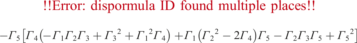
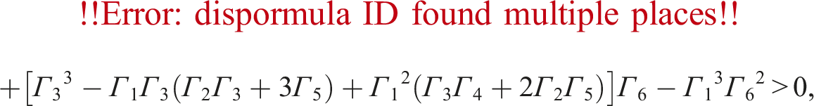
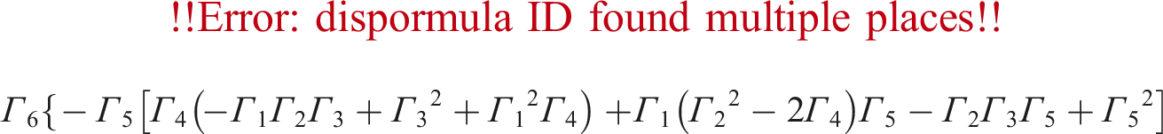
We will now outline the fundamental stability criteria that align with the RHC⁵² for certain solutions in the scenario of steady-state as in the below forms

Γ_{1} > 0, Γ_{1} Γ_{2} - Γ_{3} > 0,

Γ_{3} (Γ_{1} Γ_{2} - Γ_{3}) + Γ_{1} (Γ_{5} - Γ_{1} Γ_{4}) > 0,

Γ_{1} (Γ_{2} Γ_{3} Γ_{4} - {Γ_{2}}^{2} Γ_{5} + 2 Γ_{4} Γ_{5} - Γ_{3} Γ_{6}) + Γ_{3} (Γ_{2} Γ_{5} - Γ_{3} Γ_{4}) + {Γ_{1}}^{2} (Γ_{2} Γ_{6} - {Γ_{4}}^{2}) - {Γ_{5}}^{2} > 0,

- Γ_{5} [Γ_{4} (- Γ_{1} Γ_{2} Γ_{3} + {Γ_{3}}^{2} + {Γ_{1}}^{2} Γ_{4}) + Γ_{1} ({Γ_{2}}^{2} - 2 Γ_{4}) Γ_{5} - Γ_{2} Γ_{3} Γ_{5} + {Γ_{5}}^{2}]

+ [{Γ_{3}}^{3} - Γ_{1} Γ_{3} (Γ_{2} Γ_{3} + 3 Γ_{5}) + {Γ_{1}}^{2} (Γ_{3} Γ_{4} + 2 Γ_{2} Γ_{5})] Γ_{6} - {Γ_{1}}^{3} {Γ_{6}}^{2} > 0,

Γ_{6} {- Γ_{5} [Γ_{4} (- Γ_{1} Γ_{2} Γ_{3} + {Γ_{3}}^{2} + {Γ_{1}}^{2} Γ_{4}) + Γ_{1} ({Γ_{2}}^{2} - 2 Γ_{4}) Γ_{5} - Γ_{2} Γ_{3} Γ_{5} + {Γ_{5}}^{2}]

+ [{Γ_{3}}^{3} - Γ_{1} Γ_{3} (Γ_{2} Γ_{3} + 3 Γ_{5}) + {Γ_{1}}^{2} (Γ_{3} Γ_{4} + 2 Γ_{2} Γ_{5})] Γ_{6} - {Γ_{1}}^{3} {Γ_{6}}^{2}} > 0 .

(67)

There are numerous important advantages of applying the RHC to a vibrating dynamic system, especially when it relates to stability analysis. Here are a few main benefits:

Stability determination

The main advantage is that the RHC offer a methodical way to assess the system’s stability without having to directly solve for the characteristic equation’s roots. This is especially helpful for higher-order systems, where locating the roots can be difficult and time-consuming.

Comprehensive analysis

It makes it possible to analyze every root of the characteristic equation simultaneously, providing a comprehensive view of the stability of the system. This is important because an unstable system might result from even one root having a positive real part.

Predictive power

By using the RHC, one can predict changes in stability due to parameter variations. This is useful when designing and managing vibrating systems whose characteristics could alter over time or as a result of outside factors.

Overall, the RHC are valuable tools in the analysis and design of vibrating dynamic systems, offering a robust, efficient, and insightful means to assess and ensure stability.

The analysis of stability

This section delves into the examination of the system’s stability under consideration in utilizing the RHC of nonlinear stability. The analysis involves determining the stability parameters and conducting simulations of the system. The parameters of detuning $σ_{1}, σ_{2},$ and $σ_{3}$ along with the frequencies $w_{1}, w_{2},$ and $w_{3}$ are crucial in the stabilization process. Based on chosen parameter values, stability plots for system (65) are produced. The adjusted amplitudes $h_{1}, h_{2},$ and $h_{3}$ are drawn across distinct parametric regions, showcasing their characteristics through the trajectories of phase plane.

The potential stability and instability regions of FPs are illustrated in Figures (19)-(21) with varying values of $σ_{1}$ , showing that this range lies in the interval $σ_{1} \in [- 0.2, 0.2]$ . A closer look at Figure 19(a) reveals that at $w_{1} (= 4.47, 4.23)$ , the stable FPs fall within the area $σ_{1} \leq 0.01,$ while the unstable zones of these points exist in the region $0.01 < σ_{1}$ . Additionally, for $w_{1} = 4.08$ , the stable areas of FPs span to be in the range $σ_{1} \leq 0$ , while the unstable ones are found in the region of $0 < σ_{1}$ . The drawn solid curve and dashed one depict the stable and unstable zones of FPs, respectively.

Figure 19.

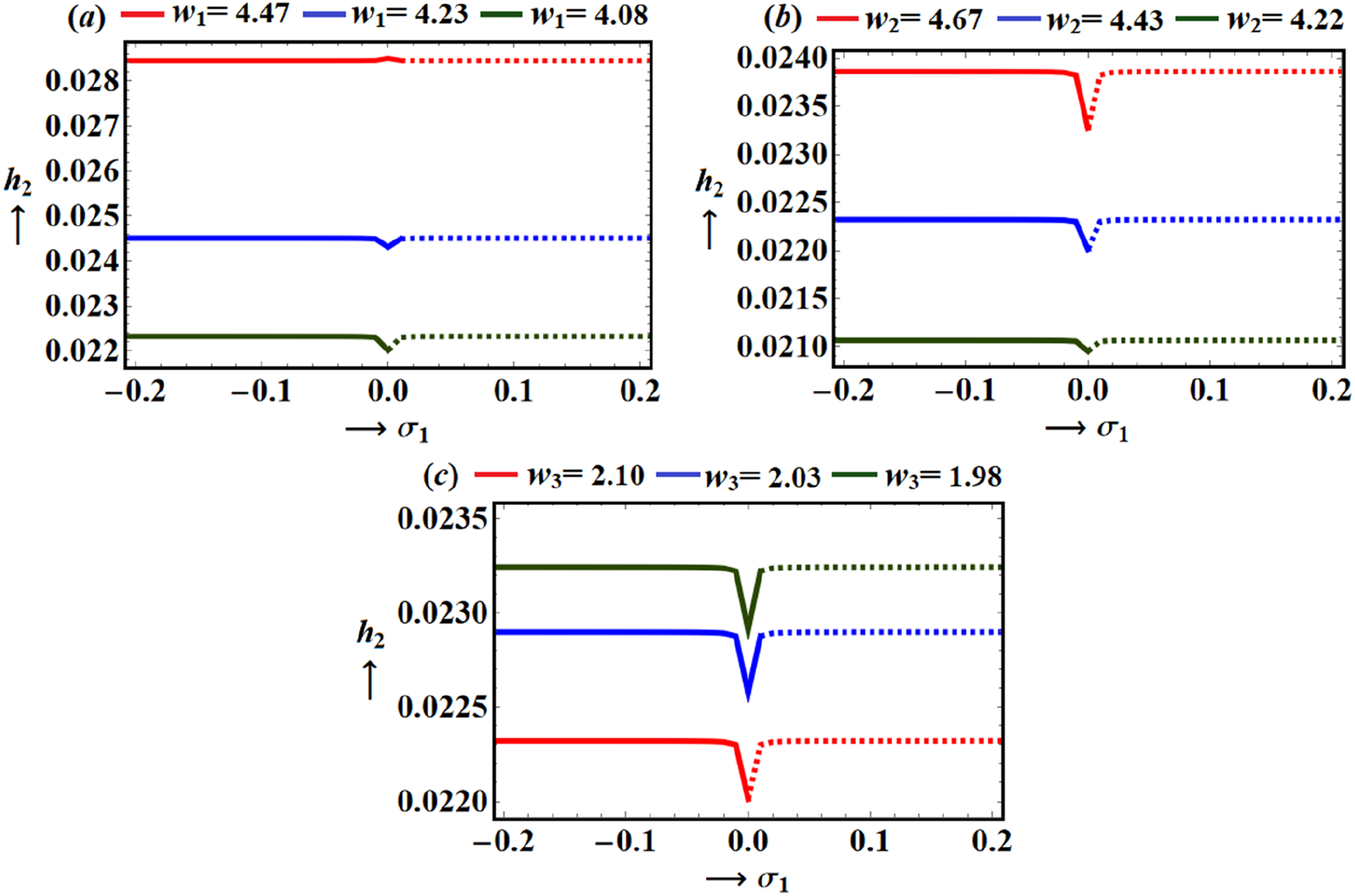
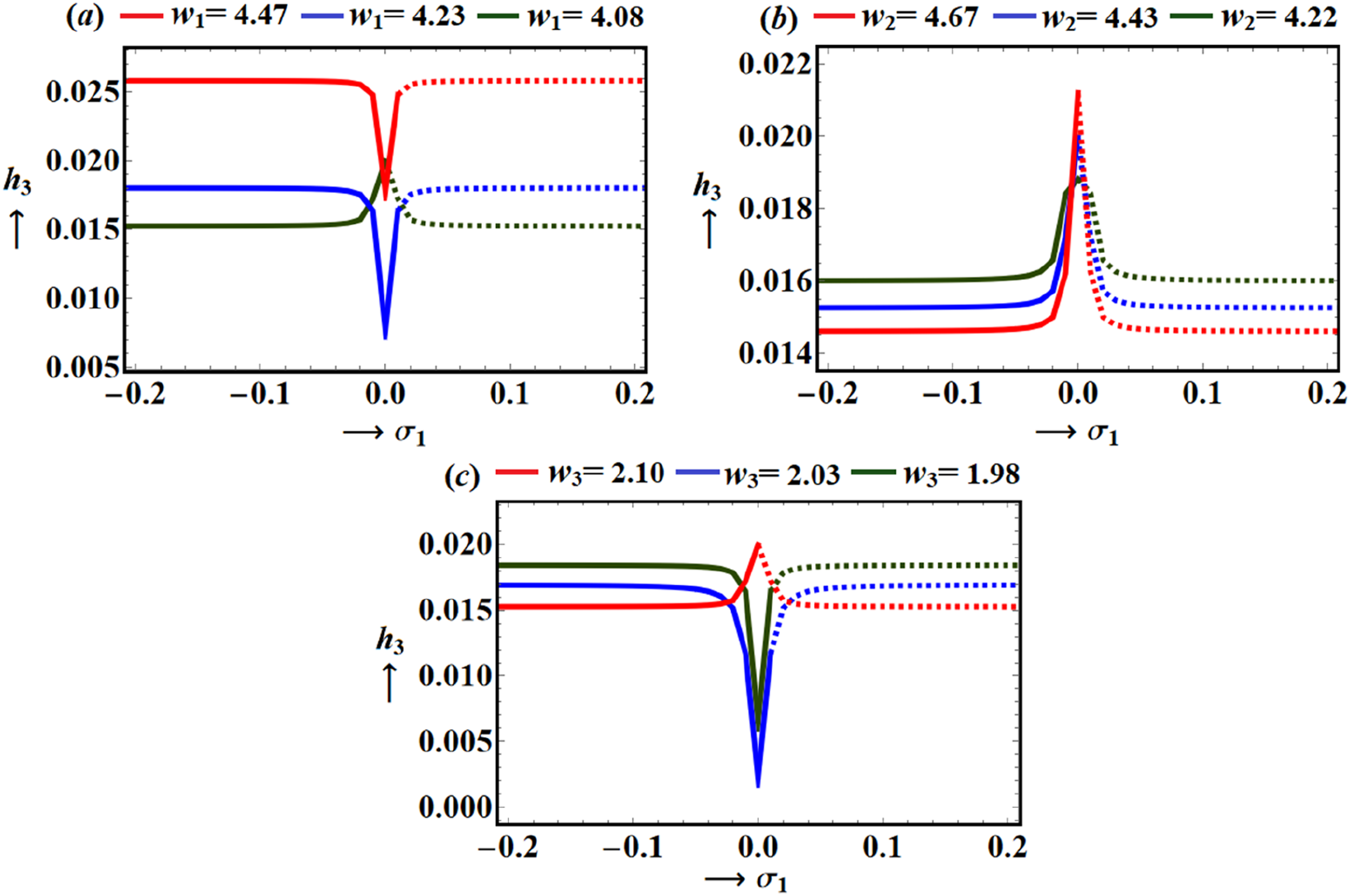
Presents the FR curves in the plane $σ_{1} h_{1}$ at $σ_{2} = p_{2} - 1,$ and $σ_{3} = p_{3} - (\frac{1}{ω_{2}})$ .

Figure 20.

Examines the fluctuation of $h_{2}$ via $σ_{1}$ at $σ_{2} = p_{2} - 1,$ and $σ_{3} = p_{3} - (\frac{1}{ω_{2}})$ .

Figure 21.

Shows the FR curves in the plane $σ_{1} h_{3}$ at $σ_{2} = p_{2} - 1,$ and $σ_{3} = p_{3} - (\frac{1}{ω_{2}})$ when: (a) $w_{1} = (4.47, 4.23, 4.08) s^{‐ 1}$ , (b) $w_{2} = (4.67, 4.43, 4.22) s^{‐ 1}$ , (c) $w_{3} = (2.10, 2.03, 1.98) s^{‐ 1}$ .

Figure 19(b) clearly demonstrates that the FPs maintain stability within the specified range of $σ_{1} \leq 0$ , yet their stability loses once $σ_{1}$ surpasses $0$ . Figures 19(c) shows that at $w_{3} = 2.10$ , the stable zones are found in the range $σ_{1} \leq 0$ , while the unstable ones are existed in the range $0 < σ_{1}$ , with a lying critical FP between the two regions. At $w_{3} (= 2.03, 1.98)$ , the stable FPs will be in the interval $σ_{1} \leq 0.01$ , and the unstable points are within $0.01 < σ_{1}$ . Based on the analysis of Figure (19), one can conclude that the amplitudes $h_{2}$ and $h_{3}$ via $σ_{1}$ demonstrate analogous patterns of stability and instability. These patterns are further illustrated in Figures (20) and (21). These figures are calculated at $σ_{2} = p_{2} - 1,$ and $σ_{3} = p_{3} - (\frac{1}{ω_{2}})$ . The critical values of the presented wave, marking the occurrence of transcritical bifurcation due to a FP, can be determined by the intersections of these curves.

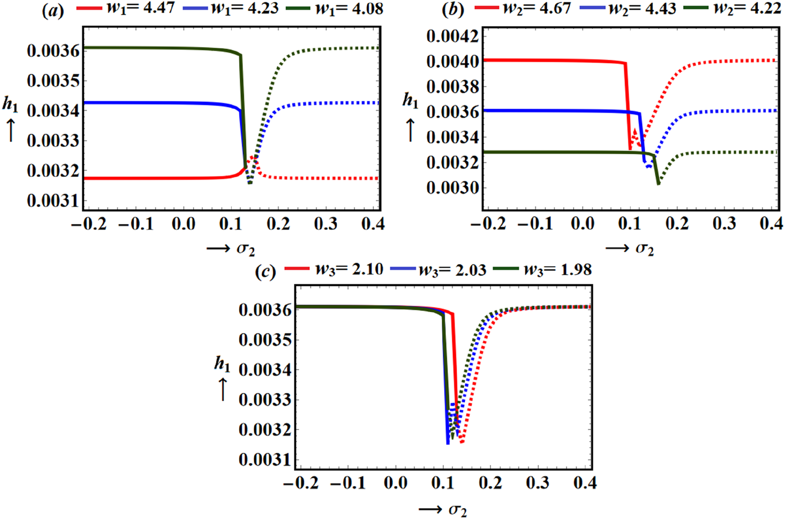
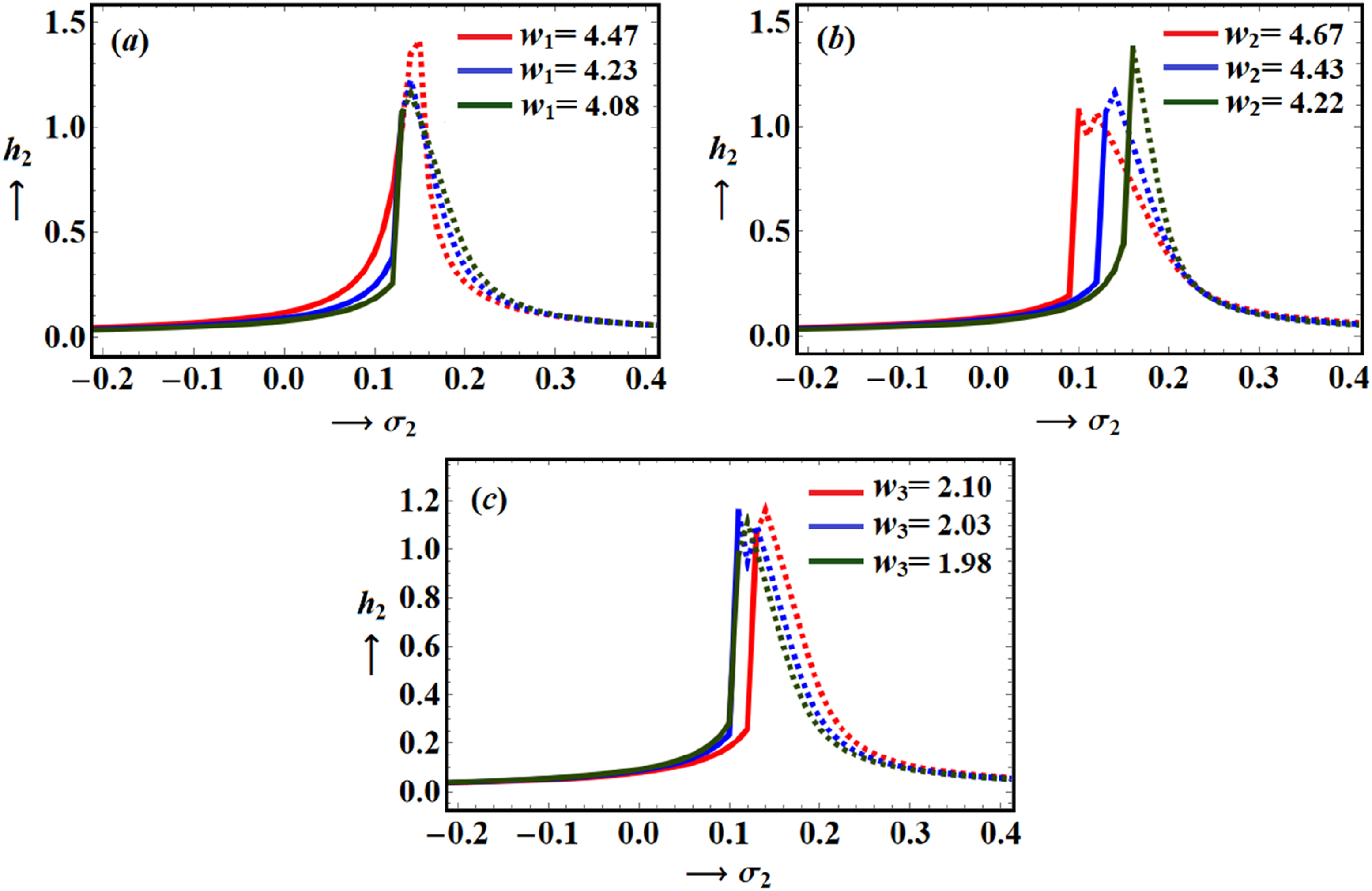
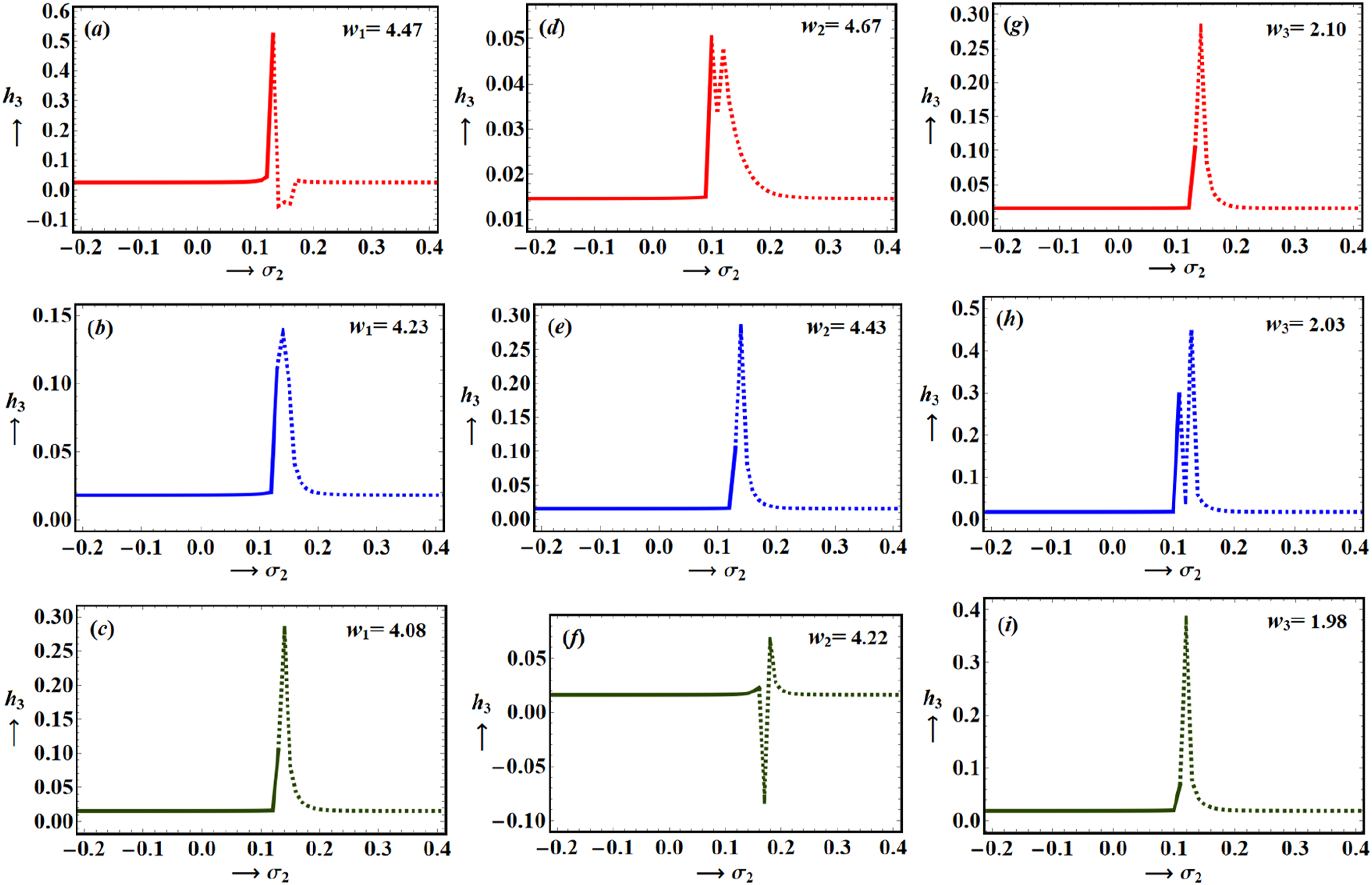
Figures (22)-(24) illustrate the changes in FR curves of $h_{1}, h_{2},$ and $h_{3}$ through the detuning parameter $σ_{2}$ for various values of $w_{j} (j = 1, 2, 3)$ ranging from $- 0.2$ to $0.4$ . The purpose of these graphs is to showcase the impact of $w_{j}$ on the FR curves of $h_{j}$ in relation to $σ_{2}$ at $σ_{1} = p_{1} - ω_{1},$ and $σ_{3} = p_{3} - (\frac{1}{ω_{2}})$ . Each curve has a single critical FP that delineates the stable and unstable regions at $w_{1} (= 4.47, 4.23, 4.08)$ , as depicted in Figure 22(a). The stable region ranges from $- 0.2$ to $0.13$ for $σ_{2}$ , while the unstable region ranges from $0.13$ to $0.4$ . Figure 22(b) reveals a critical point and three peaks when $w_{2} = 4.67$ , with stability and instability regions falling between $- 0.2$ to $0.1$ and $0.1$ to $0.4$ for $σ_{2}$ respectively. Similarly, at $w_{2} = 4.43$ , the stable region ranges from $- 0.2$ to $0.13$ for $σ_{2}$ , while the unstable region ranges from $0.13$ to $0.4$ . At $w_{2} = 4.22$ , the stable region is between $- 0.2$ to $0.16$ for $σ_{2}$ , while the unstable region is between $0.16$ to $0.4$ .

Figure 22.

Represents the FR curves in the plane $σ_{2} h_{1}$ at $σ_{1} = p_{1} - ω_{1},$ and $σ_{3} = p_{3} - (\frac{1}{ω_{2}})$ when: (a) $w_{1} = (4.47, 4.23, 4.08) s^{‐ 1}$ , (b) $w_{2} = (4.67, 4.43, 4.22) s^{‐ 1}$ , (c) $w_{3} = (2.10, 2.03, 1.98) s^{‐ 1}$ .

Figure 23.

Shows the change in $h_{2}$ versus $σ_{2}$ at $σ_{1} = p_{1} - ω_{1},$ and $σ_{3} = p_{3} - (\frac{1}{ω_{2}})$ .

Figure 24.

Depicts how the modified amplitude $h_{3}$ varies as a function of the detuning parameter $σ_{2}$ at $σ_{1} = p_{1} - ω_{1},$ and $σ_{3} = p_{3} - (\frac{1}{ω_{2}})$ .

In Figure 22(c), a single critical FP is observed at $w_{3} = 2.10$ , while the regions of stability and instability are found at $σ_{2} \leq 0.13$ and $σ_{2} > 0.13$ , respectively. On the other hand, at $w_{3} (= 2.03, 1.98)$ , the stable region zone are located at $σ_{2} \leq 0.11$ , while the unstable one is found in the range $σ_{2} > 0.11$ along with multiple peaks of FPs. Ultimately, both $h_{2}$ and $h_{3}$ display analogous stability and instability patterns concerning $σ_{2}$ , as depicted in Figures (23) and (24).

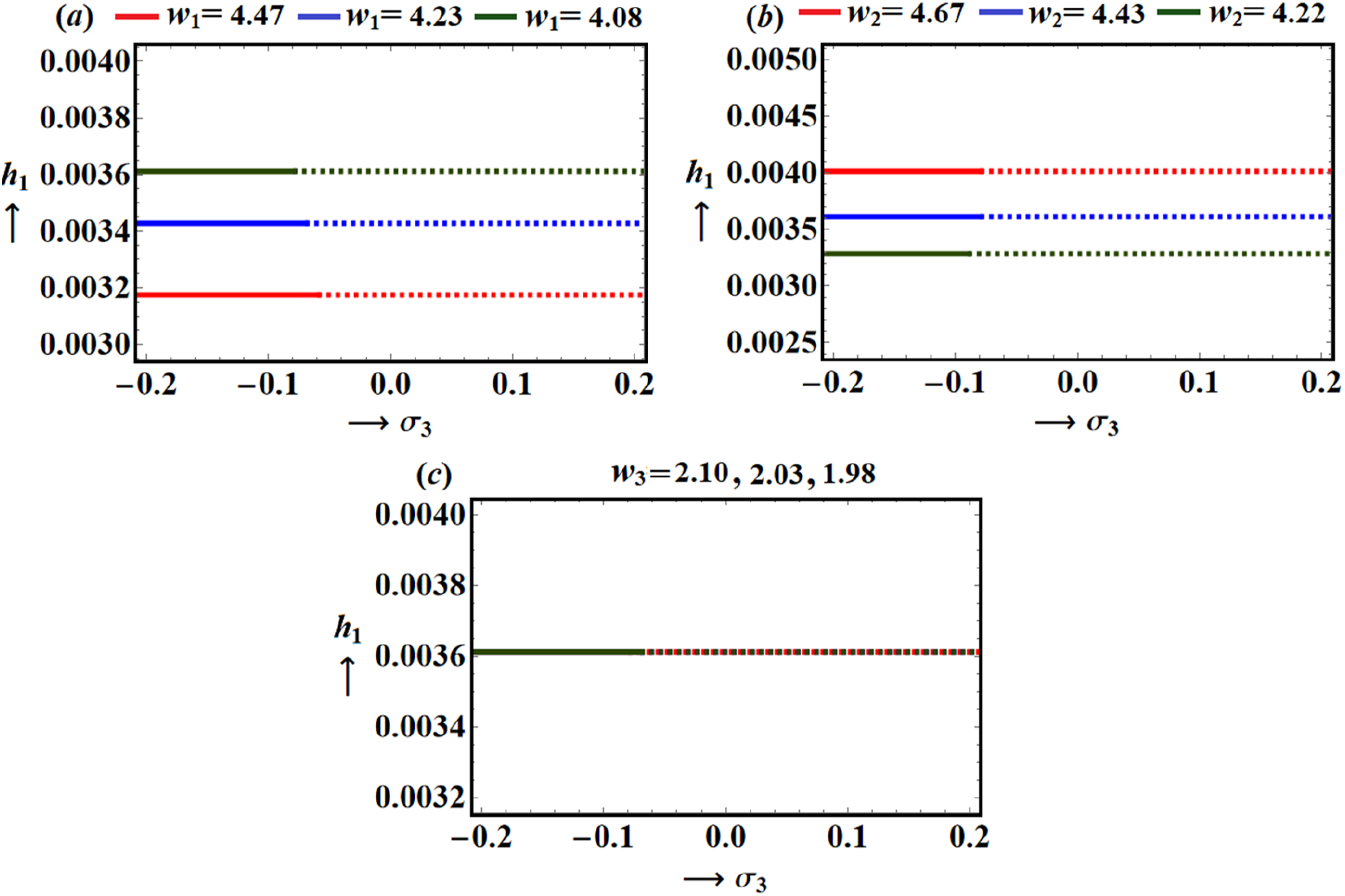
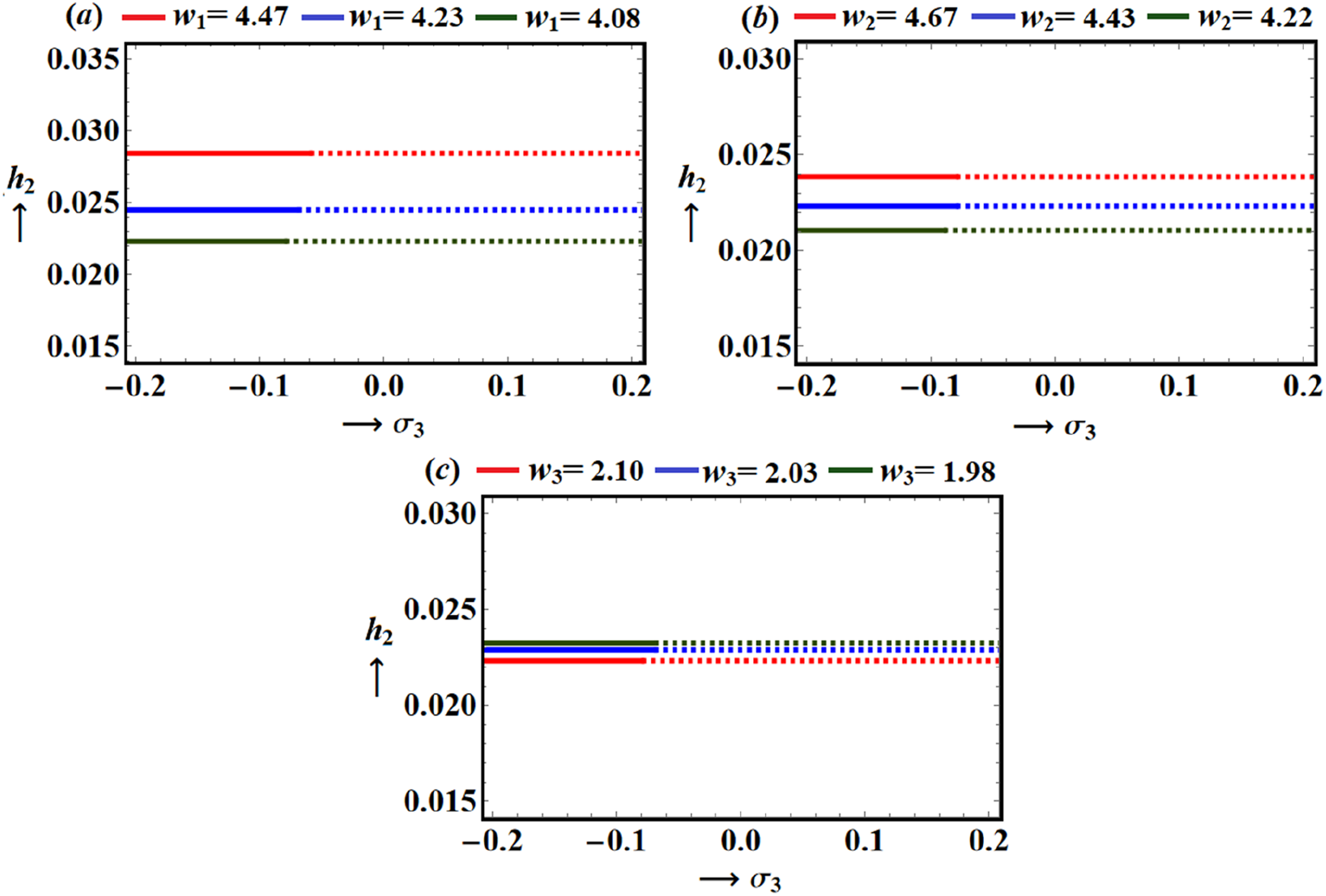
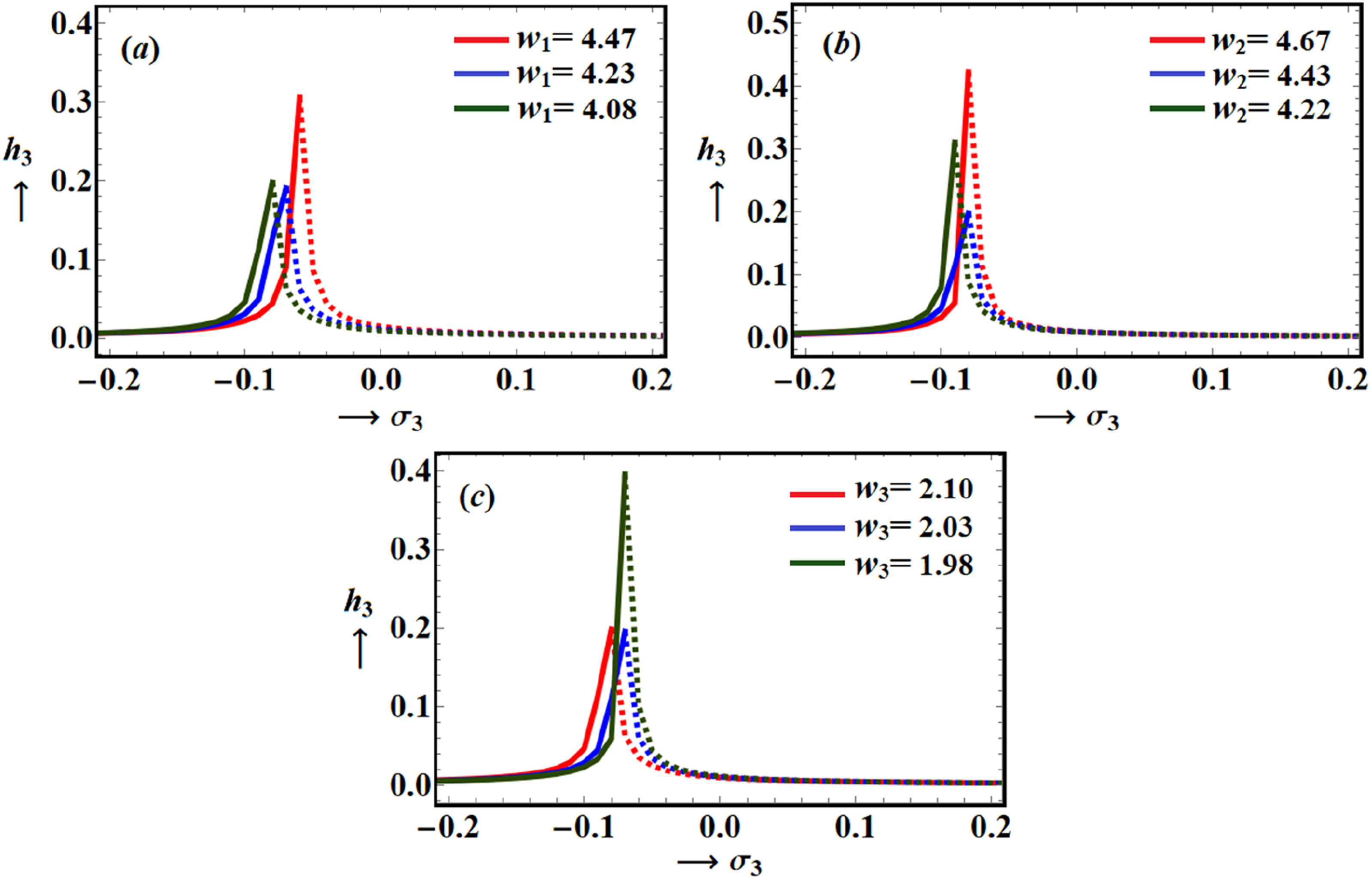
The adjusted magnitudes $h_{j}$ are plotted against $σ_{3}$ in Figures (25)-(27) to demonstrate the significant impact of $w_{j}$ on the dynamics of the system at $σ_{1} = p_{1} - ω_{1},$ and $σ_{2} = p_{2} - 1$ . The analysis focuses on the stability and instability characteristics within the range $- 0.2 \leq σ_{3} \leq 0.2$ . The behavior of the FR curves, representing the variation of $h_{1}$ via $σ_{3}$ at different values of $w_{j}$ values, is depicted as straight lines in Figure (25). According to the calculations in part (a) of Figure (25), (a) single critical FP exists, with stable and unstable FP located in the intervals $σ_{3} \leq - 0.06, σ_{3} \leq - 0.07,$ $σ_{3} \leq - 0.08,$ and $- 0.06 < σ_{3},$ $- 0.07 < σ_{3}, - 0.08 < σ_{3}$ , respectively. When $w_{2} (= 4.67, 4.43)$ , as in Figure 25(b), the FPs are stable within the range $σ_{3} \leq - 0.08,$ but lose stability in the region $- 0.08 < σ_{3}$ . Similarly, at $w_{2} = 4.22$ , stable and unstable regions occur in $σ_{3} \leq - 0.09,$ and $- 0.09 < σ_{3},$ respectively. At $w_{3} = 2.10$ , as seen in Figure 25(c), the FPs are stable in the interval $σ_{3} \leq - 0.08,$ while these points lose their stabilities in the range $- 0.08 < σ_{3}$ . Furthermore, when $w_{3} (= 2.03, 1.98)$ , only one critical and one peak FPs are observed, with stable regions existing in $σ_{3} \leq - 0.07$ and unstable regions in $- 0.07 < σ_{3}$ , respectively. Figures (26) and (27) illustrate the FR curves of $h_{2}$ and $h_{3}$ for various values of $w_{j}$ . It is important to note that the stability and instability regions depicted in these figures are consistent with those in segments of Figure (25).

Figure 25.

Shows the FR curves in the plane $σ_{3} h_{1}$ at $σ_{1} = p_{1} - ω_{1},$ and $σ_{2} = p_{2} - 1$ .

Figure 26.

Illustrates the FR curves for $h_{2}$ via $σ_{3}$ at $σ_{1} = p_{1} - ω_{1},$ and $σ_{2} = p_{2} - 1$ .

Figure 27.

Displays the frequency characteristics of $h_{3}$ via $σ_{3}$ at: (a) $w_{1} = (4.47, 4.23, 4.08) s^{‐ 1}$ , (b) $w_{2} = (4.67, 4.43, 4.22) s^{‐ 1}$ , and (c) $w_{3} = (2.10, 2.03, 1.98) s^{‐ 1}$ .

Nonlinear analysis

The investigation in this section focuses on the stability of a dynamical model utilizing nonlinear amplitudes $A_{j} (j = 1, 2, 3)$ . To examine the behavior of the nonlinear amplitude in system (55) and evaluate its stability, the following transformations will be introduced

A_{1} = \frac{1}{2} ({\tilde{U}}_{1} (τ_{2}) + i {\tilde{V}}_{1} (τ_{2})) e^{i {\tilde{σ}}_{1} τ_{2}},

A_{2} = \frac{1}{2} ({\tilde{U}}_{2} (τ_{2}) + i {\tilde{V}}_{2} (τ_{2})) e^{i {\tilde{σ}}_{2} τ_{2}},

A_{3} = \frac{1}{2} ({\tilde{U}}_{3} (τ_{2}) + i {\tilde{V}}_{3} (τ_{2})) e^{i {\tilde{σ}}_{3} τ_{2}},

U_{j} = ε {\tilde{U}}_{j}, V_{j} = ε {\tilde{V}}_{j}, σ_{j} = ε^{2} {\tilde{σ}}_{j}; (j = 1, 2, 3) .

(68)

Through the application of (55) and (68) and the subsequent isolation of the real and imaginary terms, we get

f_{1} + ω_{1} (2 \frac{d V_{1}}{d τ} + 2 σ_{1} U_{1} + c_{1} V_{1}) - \frac{3 (ω_{1}^{2} - 1)}{2 (ω_{1}^{2} - 4)} U_{1} (U_{2}^{2} + V_{2}^{2})

+ \frac{ω_{1} γ}{(α^{2} + ω_{1}^{2})} (α V_{1} - ω_{1} U_{1}) = 0,

ω_{1} (2 σ_{1} V_{1} - 2 \frac{d U_{1}}{d τ} - c_{1} U_{1}) - \frac{3 (ω_{1}^{2} - 1)}{2 (ω_{1}^{2} - 4)} V_{1} (U_{2}^{2} + V_{2}^{2}) - \frac{ω_{1} γ}{(α^{2} + ω_{1}^{2})} (α U_{1} + ω_{1} V_{1}) = 0,

f_{2} + 2 (\frac{d V_{2}}{d τ} + σ_{2} U_{2}) + c_{2} V_{2} + U_{2} [\frac{s}{(1 - ω_{2}^{2})} - \frac{3 (ω_{1}^{2} - 1)}{2 (ω_{1}^{2} - 4)} (U_{1}^{2} + V_{1}^{2})

+ \frac{(ω_{1}^{4} + 7 ω_{1}^{2} - 8)}{8 ω_{1}^{2} (ω_{1}^{2} - 4)} (U_{2}^{2} + V_{2}^{2})] = 0,

2 (σ_{2} V_{2} - \frac{d U_{2}}{d τ}) - c_{2} U_{2} + V_{2} [\frac{s}{(1 - ω_{2}^{2})} - \frac{3 (ω_{1}^{2} - 1)}{2 (ω_{1}^{2} - 4)} ({U_{1}}^{2} + {V_{1}}^{2})

+ \frac{(ω_{1}^{4} + 7 ω_{1}^{2} - 8)}{8 ω_{1}^{2} (ω_{1}^{2} - 4)} (U_{2}^{2} + V_{2}^{2})] = 0,

f_{3} + 2 ω_{2} (\frac{d V_{3}}{d τ} + σ_{3} U_{3}) + \frac{c_{3} V_{3}}{ω_{2}} + U_{3} [\frac{s}{(ω_{2}^{2} - 1)} + \frac{1}{8} (U_{3}^{2} + V_{3}^{2})

- \frac{(1 - 2 ω_{2}^{2})}{4 {(1 - ω_{2}^{2})}^{2}} (U_{2}^{2} + V_{2}^{2}) + \frac{ω_{1}^{4}}{2 (4 - ω_{1}^{2} ω_{2}^{2})} (U_{1}^{2} + V_{1}^{2})] = 0,

σ_{3} V_{3} - \frac{d U_{3}}{d τ} - \frac{1}{2 ω_{2}^{2}} c_{3} U_{3} + V_{3} [\frac{s}{2 ω_{2} (ω_{2}^{2} - 1)} + \frac{1}{16 ω_{2}} (U_{3}^{2} + V_{3}^{2})

- \frac{(1 - 2 ω_{2}^{2})}{8 ω_{2} {(1 - ω_{2}^{2})}^{2}} (U_{2}^{2} + V_{2}^{2}) + \frac{ω_{1}^{4}}{4 ω_{2} (4 - ω_{1}^{2} ω_{2}^{2})} (U_{1}^{2} + V_{1}^{2})] = 0 .

(69)

Throughout the study, the adjusted amplitudes were validated in a range of parametric areas, and their characteristics have been plotted on the phase plane curves, as demonstrated in Figures (28)-(36), utilizing the earlier data.

Figure 28.

Shows the decaying behavior of the function $U_{1} (τ)$ .

Figure 29.

Presents the decaying behavior of the function $U_{2} (τ)$ .

Figure 30.

Describes the time history of the function $U_{3}$ .

Figure 31.

Describes the variation of the function $V_{1} (τ)$ .

Figure 32.

Shows $V_{2} (τ)$ variation at various values of $w_{j}$ .

Figure 33.

The time behavior of $V_{3}$ .

Figure 34.

Shows the trajectory in phase plane $U_{1} V_{1}$ when $w_{j}$ vary.

Figure 35.

Describes the paths in the plane $U_{2} V_{2}$ when $w_{j}$ vary.

Figure 36.

Illustrates the trajectories in the plane $U_{3} V_{3}$ when $w_{j}$ vary.

The presented waves in Figures (28)-(33) illustrate the temporal evolution of the phases $U_{j}$ and $V_{j}$ via $τ$ . Thus, it can be observed that the time histories of such phases undergo fluctuations, first oscillating between growth and decline, and then stabilizing towards the end of the time period. In other words, these waves have decaying form over the examined time, where the amplitudes of these waves decrease and increase with the raise of $w_{1}$ and $w_{2}$ , respectively, as explored in Figure 28(a) and (b). Whereas there is no change in the waves’ amplitude when $w_{3}$ varies, as seen in Figure 28(c). This behavior signifies the stability of the modified amplitudes throughout the duration of the study.

One may observe an analogous behavior for the waves describing the function $U_{2} (τ)$ at various values of $w_{2}$ , as in Figure (29), with the decay of these waves being greater than those depicted in Figure (28). This implies that these waves reach a stable stage more swiftly than before. Segments of Figure (30) show decaying curves for countable waves as the adjusted phase $U_{j}$ varies with different $w_{j}$ values. The waves illustrated in Figures (31)-(32) for the functions $V_{j} (τ)$ demonstrate similar variations to those seen in Figures (28)-(30) when $w_{1}, w_{2},$ and $w_{3}$ at their specified values.

Figures (34)-(36) depict the projections of the presented trajectories in Figures (28)-(33) onto phase planes $U_{j} V_{j}$ after removing the dimensionless time $τ$ . The drawn paths in these planes have spiral shapes that converge towards a single point which showcases the stable behavior of the system under investigation.

Conclusion

This study has effectively addressed the dual objectives of reducing vibrations and harnessing energy in a 3DOF dynamical model. This model consists of a damped spring-pendulum with its pivot moving in an elliptical path at a constant angular velocity, coupled with a rigid body experiencing external harmonic forces and moments. The optimization of energy harvesting and vibration reduction has been achieved in the study by employing an electromagnetic system that utilizes the movement of a magnet within a coil. Novel, precise solutions up to the third approximation were derived in the analysis through the use of the second kind of Lagrange’s equations and the MST. Multiple resonance states were identified and scrutinized at the same time. The time evolution of solutions, along with modified phases and amplitudes, was detailed through comprehensive graphical representations, highlighting the major parameters that influence system behavior. The system’s consistent dynamics were depicted through phase portraits, and the power output and current time profiles of the electromagnetic device underscored the influence of various parameters. The stability analysis using RHC revealed a wide range of stable parameter configurations, highlighting the system’s robustness. The model’s relevance spans contemporary applications in control sensors, offering benefits across various sectors including industry, construction, automotive, transportation, and infrastructure. The contributions of this study provide important insights for enhancing the efficiency and stability of vibration reduction and energy harvesting systems in real-world scenarios.

Footnotes

Author contributions

T. S. Amer: Conceptualization, Resources, Methodology, Formal analysis, Validation, Writing- Original draft preparation, Visualization, and Reviewing.

A. M. Wahba: Resources, Methodology, Formal Analysis, Validation, Visualization and Reviewing.

A. F. Abolila: Software, Validation, Data duration, Validation, Corroboration, Rereading and Editing.

A. A. Galal: Investigation, Methodology, Data duration, Conceptualization, Validation, Reviewing and Editing.

Declaration of conflicting interests

The author(s) declared no potential conflicts of interest with respect to the research, authorship, and/or publication of this article.

Funding

The author(s) received no financial support for the research, authorship, and/or publication of this article.

ORCID iDs

TS Amer

AA Galal

Appendix I

E_{1} = [\frac{833 - ω_{2}^{2} (2499 + 2499 ω_{2}^{2} - 801 ω_{2}^{4}) + ω_{1}^{2} [1 - ω_{2}^{2} (75 + 147 ω_{2}^{2} - 81 ω_{2}^{4})]}{48 (1 - 9 ω_{2}^{2}) (ω_{1}^{2} - 4) {(ω_{2}^{2} - 1)}^{3}}],

E_{2} = \frac{ω_{2}^{2}}{(1 - ω_{2}^{2})} [\frac{i {\tilde{c}}_{3}}{ω_{2}^{2} (ω_{2}^{2} - 1)} + \frac{i {\tilde{c}}_{2}}{ω_{2}^{2} (1 - ω_{2}^{2})} + {A_{2} {\bar{A}}_{2} [1 - (ω_{1} - 1) ω_{2}] [1 + (ω_{1} - 1) ω_{2}]

\times [(ω_{1} + 1) ω_{2} - 1] [(ω_{1} + 1) ω_{2} + 1] [8 + ω_{1}^{2} - 2 (8 + ω_{1}^{2}) ω_{2}^{2} + (8 - 3 ω_{1}^{2} + ω_{1}^{4}) ω_{2}^{4}]

+ 2 ω_{1}^{2} (ω_{2}^{2} - 1) [\tilde{s} (4 - ω_{1}^{2}) [1 - 2 (ω_{1}^{2} + 1) ω_{2}^{2} + {(ω_{1}^{2} - 1)}^{2} ω_{2}^{4}] + (ω_{2}^{2} - 1)

\times {A_{3} {\bar{A}}_{3} (4 - ω_{1}^{2}) [1 - 2 (ω_{1}^{2} + 1) ω_{2}^{2} + {(ω_{1}^{2} - 1)}^{2} ω_{2}^{4}] + 2 A_{1} {\bar{A}}_{1} [3 + 4 ω_{1}^{2} + 3 ω_{1}^{4} - ω_{1}^{6}

\times 1 - 2 (ω_{1}^{2} + 1) ω_{2}^{2} + {(ω_{1}^{2} - 1)}^{2} ω_{2}^{4}},

E_{3} = {\frac{3 ω_{1}^{2} - 6 ω_{1}^{2} ω_{2}^{2} - 4 ω_{2}^{4} + 4 ω_{1}^{2} ω_{2}^{4}}{2 [1 - {(2 ω_{2} + 1)}^{2}] (ω_{1}^{2} - 4) {(ω_{2}^{2} - 1)}^{2}}}, E_{4} = {\frac{3 ω_{1}^{2} - 6 ω_{1}^{2} ω_{2}^{2} - 4 ω_{2}^{4} + 4 ω_{1}^{2} ω_{2}^{4}}{2 [1 - {(2 ω_{2} - 1)}^{2}] (ω_{1}^{2} - 4) {(ω_{2}^{2} - 1)}^{2}}},

E_{5} = {\frac{ω_{2}^{2}}{2 [1 - {(ω_{2} + 2)}^{2}] (1 - ω_{2}^{2})}}, E_{6} = {\frac{ω_{2}^{2}}{2 [1 - {(ω_{2} - 2)}^{2}] (1 - ω_{2}^{2})}},

E_{7} = ϖ \tilde{a} {\frac{ω_{1}^{2} [{(ϖ + 1)}^{2} ω_{2}^{2} - 1] - {(ϖ + 1)}^{2} (ω_{2}^{2} - 1)}{2 l (ω_{1}^{2} - ϖ^{2}) [1 - ω_{2}^{2} {(ϖ + 1)}^{2}] (ϖ + 2) (ω_{2}^{2} - 1)}},

E_{8} = ϖ \tilde{a} {\frac{ω_{1}^{2} [{(ϖ - 1)}^{2} ω_{2}^{2} - 1] - {(ϖ - 1)}^{2} (ω_{2}^{2} - 1)}{2 l (ω_{1}^{2} - ϖ^{2}) [1 - ω_{2}^{2} {(ϖ - 1)}^{2}] (ϖ - 2) (ω_{2}^{2} - 1)}},

E_{9} = \frac{1}{4 ω_{1}^{2} (2 + ω_{1}) [1 - ω_{2}^{2} {(1 + 2 ω_{1})}^{2}]} {(ω_{1} - 1) {(2 ω_{1} + 1)}^{3} - \frac{2 ω_{1}^{5}}{(ω_{2} - 1)}

+ \frac{2 ω_{1}^{5}}{(1 + ω_{2})} + \frac{2 ω_{1}^{3} {(ω_{1} + 1)}^{2}}{[(ω_{1} + 1) ω_{2} - 1]} - \frac{2 ω_{1}^{3} {(ω_{1} + 1)}^{2}}{[(ω_{1} + 1) ω_{2} + 1]}},

E_{10} = \frac{1}{4 ω_{1}^{2} (2 - ω_{1}) [1 - ω_{2}^{2} {(1 - 2 ω_{1})}^{2}]} {(ω_{1} + 1) {(2 ω_{1} - 1)}^{3} + \frac{2 ω_{1}^{5}}{(ω_{2} - 1)}

- \frac{2 ω_{1}^{5}}{(1 + ω_{2})} - \frac{2 ω_{1}^{3} {(ω_{1} - 1)}^{2}}{[(ω_{1} - 1) ω_{2} - 1]} + \frac{2 ω_{1}^{3} {(ω_{1} - 1)}^{2}}{[(ω_{1} - 1) ω_{2} + 1]}},

E_{11} = \frac{i ω_{1} ϖ^{2} \tilde{b}}{2 l (1 - ϖ^{2}) [1 - ω_{2}^{2} {(ϖ + ω_{1})}^{2}]} {\frac{ω_{1}}{(1 - ϖ^{2} ω_{2}^{2})} - 2 ϖ - \frac{ϖ^{2}}{ω_{1}} - ω_{1} - \frac{ϖ {(ϖ + ω_{1})}^{2} (2 ω_{1} + ϖ)}{ω_{1} [1 - {(ϖ + ω_{1})}^{2}]}},

E_{12} = \frac{i ω_{1} ϖ^{2} \tilde{b}}{2 l (1 - ϖ^{2}) [1 - ω_{2}^{2} {(ϖ - ω_{1})}^{2}]} {\frac{ω_{1}}{(1 - ϖ^{2} ω_{2}^{2})} + 2 ϖ - \frac{ϖ^{2}}{ω_{1}} - ω_{1} + \frac{ϖ {(ϖ - ω_{1})}^{2} (2 ω_{1} - ϖ)}{ω_{1} [1 - {(ϖ - ω_{1})}^{2}]}},

E_{13} = \frac{ω_{1}^{2} ϖ^{2} \tilde{a}}{2 l [1 - {(ϖ ω_{2} + 1)}^{2}] (ϖ^{2} - ω_{1}^{2})}, E_{14} = \frac{ω_{1}^{2} ϖ^{2} \tilde{a}}{2 l [1 - {(ϖ ω_{2} - 1)}^{2}] (ϖ^{2} - ω_{1}^{2})},

E_{15} = \frac{ω_{1}^{4}}{[1 - {(1 + ω_{1} ω_{2})}^{2}] [1 - {(1 + 2 ω_{1} ω_{2})}^{2}]}, E_{16} = \frac{ω_{1}^{4}}{[1 - {(1 - ω_{1} ω_{2})}^{2}] [1 - {(1 - 2 ω_{1} ω_{2})}^{2}]},

Appendix II

Γ_{1} = \frac{1}{2} (2 d 3 + c_{1} + c_{2} + \frac{{\sin θ}_{20} f_{2}}{h_{20}} + \frac{{\sin θ}_{10} f_{1}}{h_{10} ω_{1}} + \frac{c_{3} h_{30} + {\sin θ}_{30} f_{3} ω_{2}}{h_{30} ω_{2}^{2}}),

Γ_{2} = (8 {\sin θ}_{30} c_{3} f_{3} h_{10} h_{20} ω_{1} + h_{30} (8 {\sin θ}_{10} c_{3} f_{1} h_{20} + h_{10} (8 c_{3} ({\sin θ}_{20} f_{2}

+ (2 d 3 + c_{1} + c_{2}) h_{20}) - 3 {\cos θ}_{30} f_{3} h_{20} h_{30}) ω_{1}) ω_{2} + 8 f_{3} ({\sin θ}_{10} {\sin θ}_{30}

\times f_{1} h_{20} + h_{10} ({\sin θ}_{30} ({\sin θ}_{20} f_{2} + (2 d 3 + c_{1} + c_{2}) h_{20}) + {\cos θ}_{30} h_{20} (- d 7 h_{10}^{2}

+ d 8 h_{20}^{2} - 2 (d 9 + σ_{3}))) ω_{1}) ω_{2}^{2} + 8 h_{30} (f_{1} ({\sin θ}_{10} {\sin θ}_{20} f_{2} + h_{20} ({\sin θ}_{10}

\times (2 d 3 + c_{1} + c_{2}) + {\cos θ}_{10} (2 d 1 + d 2 h_{20}^{2} - 2 σ_{1}))) + h_{10} ((2 d 3 + c_{1}) c_{2} h_{20}

+ f_{2} ({\sin θ}_{20} (2 d 3 + c_{1} + c_{2}) + {\cos θ}_{20} (d 4 h_{10}^{2} - 2 (d 5 + d 6 h_{20}^{2} + σ_{2}))))

\times ω_{1}) ω_{2}^{3}) / (32 h_{10} h_{20} h_{30} ω_{1} ω_{2}^{3}),

Γ_{3} = (8 c_{3} ({\sin θ}_{30} f_{3} ({\sin θ}_{10} f_{1} h_{20} + h_{10} ({\sin θ}_{20} f_{2} + (2 d 3 + c_{1} + c_{2}) h_{20}) ω_{1})

+ h_{30} ({\sin θ}_{10} f_{1} ({\sin θ}_{20} f_{2} + (2 d 3 + c_{1} + c_{2}) h_{20}) + {\cos θ}_{10} f_{1} h_{20} (2 d 1

+ d 2 h_{20}^{2} - 2 σ_{1}) + h_{10} ((2 d 3 + c_{1}) c_{2} h_{20} + f_{2} ({\sin θ}_{20} (2 d 3 + c_{1} + c_{2})

+ {\cos θ}_{20} (d 4 h_{10}^{2} - 2 (d 5 + d 6 h_{20}^{2} + σ_{2})))) ω_{1}) ω_{2}) + ω_{2} (3 {\cos θ}_{30} f_{3} h_{30}^{2}

\times (- {\sin θ}_{10} f_{1} h_{20} - h_{10} ({\sin θ}_{20} f_{2} + (2 d 3 + c_{1} + c_{2}) h_{20}) ω_{1})

+ 4 f_{3} (- 2 {\cos θ}_{30} (d 7 h_{10}^{2} - d 8 h_{20}^{2} + 2 (d 9 + σ_{3})) ({\sin θ}_{10} f_{1} h_{20} + h_{10} ({\sin θ}_{20} f_{2}

+ (2 d 3 + c_{1} + c_{2}) h_{20}) ω_{1}) + 2 {\sin θ}_{30} ({\sin θ}_{10} f_{1} ({\sin θ}_{20} f_{2} + (2 d 3 + c_{1} + c_{2}) h_{20})

+ {\cos θ}_{10} f_{1} h_{20} (2 d 1 + d 2 h_{20}^{2} - 2 σ_{1}) + h_{10} ((2 d 3 + c_{1}) c_{2} h_{20}

+ f_{2} ({\sin θ}_{20} (2 d 3 + c_{1} + c_{2}) + {\cos θ}_{20} (d 4 h_{10}^{2} - 2 (d 5 + d 6 h_{20}^{2} + σ_{2}))))

\times ω_{1})) ω_{2} + 8 h_{30} (c_{2} f_{1} h_{20} ({\sin θ}_{10} (2 d 3 + c_{1}) + {\cos θ}_{10} (2 d 1 + d 2 h_{20}^{2} - 2 σ_{1}))

- {\cos θ}_{20} f_{2} (- d 4 h_{10}^{2} + 2 (d 5 + d 6 h_{20}^{2} + σ_{2})) ({\sin θ}_{10} f_{1} + (2 d 3 + c_{1}) h_{10} ω_{1})

+ {\sin θ}_{20} f_{2} (f_{1} ({\sin θ}_{10} (2 d 3 + c_{1} + c_{2}) + {\cos θ}_{10} (2 d 1 + d 2 h_{20}^{2} - 2 σ_{1}))

+ (2 d 3 + c_{1}) c_{2} h_{10} ω_{1})) ω_{2}^{2})) / (64 h_{10} h_{20} h_{30} ω_{1} ω_{2}^{3}),

Γ_{4} = (8 c_{3} (h_{10} ω_{1} ({\sin θ}_{30} (2 d 3 + c_{1}) c_{2} f_{3} h_{20} + {\cos θ}_{20} f_{2} (d 4 h_{10}^{2} - 2 (d 5

+ d 6 h_{20}^{2} + σ_{2})) ({\sin θ}_{30} f_{3} + (2 d 3 + c_{1}) h_{30} ω_{2}) + {\sin θ}_{20} f_{2} ({\sin θ}_{30}

\times (2 d 3 + c_{1} + c_{2}) f_{3} + (2 d 3 + c_{1}) c_{2} h_{30} ω_{2})) + f_{1} (f_{2} ({\sin θ}_{10} {\sin θ}_{20}

\times {\sin θ}_{30} f_{3} + h_{30} ({\sin θ}_{20} ({\sin θ}_{10} (2 d 3 + c_{1} + c_{2}) + {\cos θ}_{10}

\times (2 d 1 + d 2 h_{20}^{2} - 2 σ_{1})) + {\cos θ}_{20} {\sin θ}_{10} (d 4 h_{10}^{2} - 2 (d 5 + d 6 h_{20}^{2} + σ_{2})))

\times ω_{2}) + h_{20} ({\cos θ}_{10} (2 d 1 + d 2 h_{20}^{2} - 2 σ_{1}) ({\sin θ}_{30} f_{3} + c_{2} h_{30} ω_{2})

+ {\sin θ}_{10} ({s i n θ}_{30} (2 d 3 + c_{1} + c_{2}) f_{3} + (2 d 3 + c_{1}) c_{2} h_{30} ω_{2}))))

+ ω_{2} (f_{3} h_{10} ω_{1} (8 {\sin θ}_{30} (2 d 3 + c_{1}) f_{2} ({\sin θ}_{20} c_{2} + {\cos θ}_{20} (d 4 h_{10}^{2}

- 2 (d 5 + d 6 h_{20}^{2} + σ_{2}))) ω_{2} - {\cos θ}_{30} ((2 d 3 + c_{1}) c_{2} h_{20} + f_{2} ({\sin θ}_{20}

\times (2 d 3 + c_{1} + c_{2}) + {\cos θ}_{20} (d 4 h_{10}^{2} - 2 (d 5 + d 6 h_{20}^{2} + σ_{2})))) (3 h_{30}^{2}

+ 8 (d 7 h_{10}^{2} - d 8 h_{20}^{2} + 2 (d 9 + σ_{3})) ω_{2})) + f_{1} (f_{2} (8 h_{30} ({\sin θ}_{10} (2 d 3 + c_{1})

\times ({\sin θ}_{20} c_{2} + {\cos θ}_{20} (d 4 h_{10}^{2} - 2 (d 5 + d 6 h_{20}^{2} + σ_{2}))) + {\cos θ}_{10}

\times ({\sin θ}_{20} c_{2} (2 d 1 + d 2 h_{20}^{2} - 2 σ_{1}) - {\cos θ}_{20} (d 4 h_{10}^{2} (- 2 d 1 + 3 d 2 h_{20}^{2}

+ 2 σ_{1}) + 2 (2 d 1 + d 2 h_{20}^{2} - 2 σ_{1}) (d 5 + d 6 h_{20}^{2} + σ_{2})))) ω_{2}^{2} + f_{3} (- 3

\times {\cos θ}_{30} {\sin θ}_{10} {\sin θ}_{20} h_{30}^{2} - 8 (2 d 9 {\cos θ}_{30} {\sin θ}_{10} {\sin θ}_{20} + 2 (d 5 {\cos θ}_{20}

\times {\sin θ}_{10} - (d 1 {\cos θ}_{10} + d 3 {\sin θ}_{10}) {\sin θ}_{20}) {\sin θ}_{30} - {\sin θ}_{10} {\sin θ}_{20}

\times {\sin θ}_{30} c_{1} - {\sin θ}_{10} {\sin θ}_{20} {\sin θ}_{30} c_{2} + d 7 {\cos θ}_{30} {\sin θ}_{10} {\sin θ}_{20} h_{10}^{2}

- d 4 {\cos θ}_{20} {\sin θ}_{10} {\sin θ}_{30} h_{10}^{2} - d 8 {\cos θ}_{30} {\sin θ}_{10} {\sin θ}_{20} h_{20}^{2}

+ 2 d 6 {\cos θ}_{20} {\sin θ}_{10} {\sin θ}_{30} h_{20}^{2} - d 2 {\cos θ}_{10} {\sin θ}_{20} {\sin θ}_{30} h_{20}^{2}

+ 2 {\cos θ}_{10} {\sin θ}_{20} {\sin θ}_{30} σ_{1} + 2 {\cos θ}_{20} {\sin θ}_{10} {\sin θ}_{30} σ_{2}

+ 2 {\cos θ}_{30} {\sin θ}_{10} {\sin θ}_{20} σ_{3}) ω_{2})) + f_{3} h_{20} (8 {\sin θ}_{30} c_{2} ({\sin θ}_{10}

\times (2 d 3 + c_{1}) + {\cos θ}_{10} (2 d 1 + d 2 h_{20}^{2} - 2 σ_{1})) ω_{2} - {\cos θ}_{30} ({\sin θ}_{10}

\times (2 d 3 + c_{1} + c_{2}) + {\cos θ}_{10} (2 d 1 + d 2 h_{20}^{2} - 2 σ_{1})) (3 h_{30}^{2} + 8 (d 7 h_{10}^{2}

- d 8 h_{20}^{2} + 2 (d 9 + σ_{3})) ω_{2}))))) / (128 h_{10} h_{20} h_{30} ω_{1} ω_{2}^{3}),

Γ_{5} = (f_{3} ω_{2} (6 d 5 {\cos θ}_{20} {\cos θ}_{30} {\sin θ}_{10} f_{1} f_{2} h_{30}^{2} - 6 d 1 {\cos θ}_{10} {\cos θ}_{30}

\times {\sin θ}_{20} f_{1} f_{2} h_{30}^{2} - 6 d 3 {\cos θ}_{30} {\sin θ}_{10} {\sin θ}_{20} f_{1} f_{2} h_{30}^{2} - 3 {\cos θ}_{30}

\times {\sin θ}_{10} {\sin θ}_{20} c_{1} f_{1} f_{2} h_{30}^{2} - 3 {\cos θ}_{30} {\sin θ}_{10} {\sin θ}_{20} c_{2} f_{1} f_{2} h_{30}^{2}

- 3 d 4 {\cos θ}_{20} {\cos θ}_{30} {\sin θ}_{10} f_{1} f_{2} h_{10}^{2} h_{30}^{2} - 6 d 1 {\cos θ}_{10} {\cos θ}_{30} c_{2}

\times f_{1} h_{20} h_{30}^{2} - 6 d 3 {\cos θ}_{30} {\sin θ}_{10} c_{2} f_{1} h_{20} h_{30}^{2} - 3 {\cos θ}_{30} {\sin θ}_{10} c_{1} c_{2}

\times f_{1} h_{20} h_{30}^{2} + 6 d 6 {\cos θ}_{20} {\cos θ}_{30} {\sin θ}_{10} f_{1} f_{2} h_{20}^{2} h_{30}^{2} - 3 d 2 {\cos θ}_{10}

\times {\cos θ}_{30} {\sin θ}_{20} f_{1} f_{2} h_{20}^{2} h_{30}^{2} - 3 d 2 {\cos θ}_{10} {\cos θ}_{30} c_{2} f_{1} h_{20}^{3} h_{30}^{2}

+ 6 {\cos θ}_{10} {\cos θ}_{30} {\sin θ}_{20} f_{1} f_{2} h_{30}^{2} σ_{1} + 6 {\cos θ}_{10} {\cos θ}_{30} c_{2} f_{1} h_{20} h_{30}^{2} σ_{1}

+ 6 {\cos θ}_{20} {\cos θ}_{30} {\sin θ}_{10} f_{1} f_{2} h_{30}^{2} σ_{2} + 12 d 3 d 5 {\cos θ}_{20} {\cos θ}_{30} f_{2} h_{10} h_{30}^{2} ω_{1}

+ 6 d 5 {\cos θ}_{20} {\cos θ}_{30} c_{1} f_{2} h_{10} h_{30}^{2} ω_{1} - 6 d 3 {\cos θ}_{30} {\sin θ}_{20} c_{2} f_{2} h_{10} h_{30}^{2} ω_{1}

- 3 {\cos θ}_{30} {\sin θ}_{20} c_{1} c_{2} f_{2} h_{10} h_{30}^{2} ω_{1} - 6 d 3 d 4 {\cos θ}_{20} {\cos θ}_{30} f_{2} h_{10}^{3} h_{30}^{2} ω_{1}

- 3 d 4 {\cos θ}_{20} {\cos θ}_{30} c_{1} f_{2} h_{10}^{3} h_{30}^{2} ω_{1} + 12 d 3 d 6 {\cos θ}_{20} {\cos θ}_{30} f_{2} h_{10} h_{20}^{2} h_{30}^{2} ω_{1}

+ 6 d 6 {\cos θ}_{20} {\cos θ}_{30} c_{1} f_{2} h_{10} h_{20}^{2} h_{30}^{2} ω_{1} + 12 d 3 {\cos θ}_{20} {\cos θ}_{30} f_{2} h_{10} h_{30}^{2} σ_{2} ω_{1}

+ 6 {\cos θ}_{20} {\cos θ}_{30} c_{1} f_{2} h_{10} h_{30}^{2} σ_{2} ω_{1} + 4 (2 {\sin θ}_{30} f_{1} f_{2} ({\sin θ}_{10} (2 d 3 + c_{1})

\times ({\sin θ}_{20} c_{2} + {\cos θ}_{20} (d 4 h_{10}^{2} - 2 (d 5 + d 6 h_{20}^{2} + σ_{2}))) + {\cos θ}_{10} ({\sin θ}_{20}

\times c_{2} (2 d 1 + d 2 h_{20}^{2} - 2 σ_{1}) - {\cos θ}_{20} (d 4 h_{10}^{2} (- 2 d 1 + 3 d 2 h_{20}^{2} + 2 σ_{1})

+ 2 (2 d 1 + d 2 h_{20}^{2} - 2 σ_{1}) (d 5 + d 6 h_{20}^{2} + σ_{2})))) + 2 {\cos θ}_{30} (f_{1} ({\cos θ}_{10}

\times ({\sin θ}_{20} f_{2} + c_{2} h_{20}) (2 d 1 + d 2 h_{20}^{2} - 2 σ_{1}) + {\sin θ}_{10} ((2 d 3 + c_{1}) c_{2} h_{20}

+ f_{2} ({\sin θ}_{20} (2 d 3 + c_{1} + c_{2}) + {\cos θ}_{20} (d 4 h_{10}^{2} - 2 (d 5 + d 6 h_{20}^{2} + σ_{2})))))

\times (- d 7 h_{10}^{2} + d 8 h_{20}^{2} - 2 (d 9 + σ_{3})) - (2 d 3 + c_{1}) f_{2} h_{10} ({\sin θ}_{20} c_{2} + {\cos θ}_{20}

\times (d 4 h_{10}^{2} - 2 (d 5 + d 6 h_{20}^{2} + σ_{2}))) (d 7 h_{10}^{2} - d 8 h_{20}^{2} + 2 (d 9 + σ_{3})) ω_{1})) ω_{2})

- 8 c_{3} ({\sin θ}_{30} (2 d 3 + c_{1}) f_{2} f_{3} h_{10} (- {\sin θ}_{20} c_{2} + {\cos θ}_{20} (- d 4 h_{10}^{2}

+ 2 (d 5 + d 6 h_{20}^{2} + σ_{2}))) ω_{1} + f_{1} (- {\sin θ}_{30} c_{2} f_{3} h_{20} ({\sin θ}_{10} (2 d 3 + c_{1})

+ {\cos θ}_{10} (2 d 1 + d 2 h_{20}^{2} - 2 σ_{1})) + f_{2} ({s i n θ}_{30} f_{3} ({\sin θ}_{20} (- {\sin θ}_{10}

\times (2 d 3 + c_{1} + c_{2}) - {\cos θ}_{10} (2 d 1 + d 2 h_{20}^{2} - 2 σ_{1})) + {\cos θ}_{20} {\sin θ}_{10}

\times (- d 4 h_{10}^{2} + 2 (d 5 + d 6 h_{20}^{2} + σ_{2}))) + h_{30} ({\sin θ}_{10} (2 d 3 + c_{1}) (- {\sin θ}_{20} c_{2}

+ {\cos θ}_{20} (- d 4 h_{10}^{2} + 2 (d 5 + d 6 h_{20}^{2} + σ_{2}))) + {\cos θ}_{10} (- {\sin θ}_{20} c_{2} (2 d 1

+ d 2 h_{20}^{2} - 2 σ_{1}) + {\cos θ}_{20} (d 4 h_{10}^{2} (- 2 d 1 + 3 d 2 h_{20}^{2} + 2 σ_{1}) + 2 (2 d 1 + d 2 h_{20}^{2}

- 2 σ_{1}) (d 5 + d 6 h_{20}^{2} + σ_{2})))) ω_{2})))) / (256 h_{10} h_{20} h_{30} ω_{1} ω_{2}^{3}),

Γ_{6} = (f_{1} f_{2} f_{3} ({\sin θ}_{10} (2 d 3 + c_{1}) (- {\sin θ}_{20} c_{2} + {\cos θ}_{20} (- d 4 h_{10}^{2}

+ 2 (d 5 + d 6 h_{20}^{2} + σ_{2}))) + {\cos θ}_{10} (- {\sin θ}_{20} c_{2} (2 d 1 + d 2 h_{20}^{2} - 2 σ_{1})

+ {\cos θ}_{20} (d 4 h_{10}^{2} (- 2 d 1 + 3 d 2 h_{20}^{2} + 2 σ_{1}) + 2 (2 d 1 + d 2 h_{20}^{2} - 2 σ_{1}) (d 5

+ d 6 h_{20}^{2} + σ_{2})))) (- 8 {\sin θ}_{30} c_{3} + {\cos θ}_{30} ω_{2} (3 h_{30}^{2} + 8 (d 7 h_{10}^{2} - d 8 h_{20}^{2}

+ 2 (d 9 + σ_{3})) ω_{2}))) / (512 h_{10} h_{20} h_{30} ω_{1} ω_{2}^{3}),

where

d 1 = \frac{ω_{1} γ}{2 (α^{2} + ω_{1}^{2})}, d 5 = \frac{s}{2 (1 - ω_{2}^{2})},

d 2 = \frac{3 (ω_{1}^{2} - 1)}{2 ω_{1} (ω_{1}^{2} - 4)}, d 6 = \frac{3 (ω_{1}^{4} + 7 ω_{1}^{2} - 8)}{16 ω_{1}^{2} (ω_{1}^{2} - 4)},

d 3 = \frac{α γ}{2 (α^{2} + ω_{1}^{2})}, d 7 = \frac{ω_{1}^{4}}{2 ω_{2} (4 - ω_{1}^{2} ω_{2}^{2})},

d 4 = \frac{3 (ω_{1}^{2} - 1)}{2 (ω_{1}^{2} - 4)}, d 8 = \frac{(1 - 2 ω_{2}^{2})}{4 ω_{2} {(1 - ω_{2}^{2})}^{2}},

d 9 = \frac{s}{2 ω_{2} (ω_{2}^{2} - 1)} .

References

Nath

Debnath

Choudhury

. Methods for improving the Seismic performance of structures - a review. Mater. Sci. Eng 2018; 377(1): 012141.

Muralt

. Ferroelectric thin films for micro-sensors and actuators: a review. J Micromech Microeng 2000; 10(2): 136–146.

Zhou

Liao

. Analysis and design of a self-powered piezoelectric microaccelerometer. Proc SPIE 2005; 5763: 233–240. Bellingham.

Paradiso

Starner

. Energy scavenging for mobile and wireless electronics. IEEE ComSoc 2005; 4(1): 18–27.

Mizuno

Chetwynd

. Investigation of a resonance microgenerator. J Micromech Microeng 2003; 13(2): 209–216.

Mitcheson

Yeatman

Rao

, et al. Energy harvesting from human and machine motion for wireless electronic devices. Proc IEEE 2008; 96(9): 1457–1486.

Naruse

Matsubara

Mabuchi

, et al. Electrostatic micro power generation from low-frequency vibration such as human motion. J Micromech Microeng 2009; 19(9): 094002.

Tsutsumino

Suzuki

Kasagi

, et al. Seismic power generator using high performance polymer electrets. In Proc. of IEEE MEMS. Istanbul, Turkey, 2006, pp. 98–101.

Suzuki

Edamoto

Kasagi

, et al. Micro electret energy harvesting device with analogue impedance conversion circuit. Proc. Power MEMS 2008; 8: 7–10.

10.

. Low-frequency piezoelectric energy harvesting prototype suitable for the MEMS implementation. Microelectro. J 2011; 42(2): 277–282.

11.

Galchev

Aktakka

Kim

, et al. A piezoelectric frequency-increased power generator for scavenging low-frequency ambient vibration. Proc. Of MEMS. Hong Kong 2010: 1203–1206.

12.

Jonnalagadda

, Magnetic induction systems to harvest energy from mechanical vibrations (MSc Thesis), M. I. T. Massachusetts; 2007.

13.

Nia

Zawawi

NAWA

Singh

BSM

. A review of walking energy harvesting using piezoelectric materials. IOP Conf Ser Mater Sci Eng 2017; 291(1): 012026.

14.

Tran

Ghayesh

Arjomandi

. Ambient vibration energy harvesters: a review on non-linear techniques for performance enhancement. Int J Eng Sci 2018; 127: 162–185.

15.

Tao

Lye

Miao

, et al. Design and implementation of an out-of-plane electrostatic vibration energy harvester with dual-charged electret plates. Microelectron Eng 2015; 135: 32–37.

16.

Abdelkefi

Barsallo

Tang

, et al. Modeling, validation, and performance of low-frequency piezoelectric energy harvesters. J Intell Mater Syst Struct 2014; 25(12): 1429–1444.

17.

Jiang

Han

Chen

, et al. Improving energy harvesting by internal resonance in a spring-pendulum system. Acta Mech Sin 2020; 36: 618–623.

18.

Amer

Tian

, et al. Controlling the kinematics of a spring-pendulum system using an energy harvesting device. Noise Vibr 2022; 41(3): 1234–1257.

19.

Abohamer

Awrejcewicz

Starosta

, et al. Influence of the motion of a spring pendulum on energy-harvesting devices. Appl Sci 2021; 11(18): 8658.

20.

Pan

Qin

Deng

, et al. Harvesting weak vibration energy by integrating piezoelectric inverted beam and pendulum. Energy (Oxf.) 2021; 227(120374): 120374.

21.

Dotti

Sosa

. Pendulum systems for harvesting vibration energy from railroad tracks and sleepers during the passage of a high-speed train: a feasibility evaluation. Theor. Appl. Mech. Lett 2019; 9(4): 229–235.

22.

Kumar

Gupta

Ali

. Energy harvesting from chaos in base excited double pendulum. Mech Syst Signal Process 2019; 124: 49–64.

23.

Kuang

Hide

Zhu

. Broadband energy harvesting by nonlinear magnetic rolling pendulum with subharmonic resonance. Appl Energy 2019; 255(113822): 113822.

24.

Fan

Zhu

, et al. Predicting energy harvesting performance of a random nonlinear dielectric elastomer pendulum. Appl Energy 2021; 289(116696): 116696.

25.

Cai

Zhu

. Applying double-mass pendulum oscillator with tunable ultra-low frequency in wave energy converters. Appl Energy 2021; 298(117228): 117228.

26.

Wijata

Polczyński

Awrejcewicz

. Theoretical and numerical analysis of regular one-side oscillations in a single pendulum system driven by a magnetic field. Mech Syst Signal Process 2021; 150(107229): 107229.

27.

Abohamer

Awrejcewicz

Amer

. Modeling of the vibration and stability of a dynamical system coupled with an energy harvesting device. Alex Eng J 2023; 63: 377–397.

28.

Amer

Arab

Galal

. On the influence of an energy harvesting device on a dynamical system, Low Freq. Noise Vibr 2024; 3: 14613484231224588.

29.

Kęci

. Energy harvesting of a pendulum vibration absorber. Przeglad Elektrotechniczny 2013; 89(7): 169–172.

30.

Kecik

Brzeski

Perlikowski

. Non-Linear dynamics and optimization of a harvester-absorber system. Int J Str Stab Dyn 2017; 17(5): 1740001.

31.

Kecik

. Assessment of energy harvesting and vibration mitigation of a pendulum dynamic absorber. Mech Syst Signal Process 2018; 106: 198–209.

32.

Kecik

Mitura

. Energy recovery from a pendulum tuned mass damper with two independent harvesting sources. Int J Mech Sci 2020; 174: 105568.

33.

Wang

Yang

. Nonlinear multi-modal energy harvester and vibration absorber using magnetic softening spring. J Sound Vib 2020; 476: 115332.

34.

Kecik

. Numerical study of a pendulum absorber/harvester system with a semi‐active suspension. Z Angew Math Mech 2021; 101(1): e202000045.

35.

Kecik

. Simultaneous vibration mitigation and energy harvesting from a pendulum-type absorber. Commun Nonlinear Sci Numer Simul 2021; 92: 105479.

36.

Zhang

Sorokin

. Energy harvesting using a novel autoparametric pendulum absorber-harvester. J Sound Vib 2021; 499: 116014.

37.

Kecik

Mitura

. Theoretical and experimental investigations of a pseudo-magnetic levitation system for energy harvesting. Sens 2020; 20(6): 1623.

38.

Hosseinkhani

Younesian

Eghbali

, et al. Sound and vibration energy harvesting for railway applications: a review on linear and nonlinear techniques. Energy Rep 2021; 7: 852–874.

39.

Amer

Moatimid

Amer

. Dynamical stability of a 3-DOF auto-parametric vibrating system. J Vib Eng Technol 2023; 11: 4151–4186.

40.

Strogatz

. Nonlinear dynamics and chaos: with applications to Physics, Biology, Chemistry and engineering. CRC Press, 2015.

41.

Abohamer

Awrejcewicz

Amer

. Modeling and analysis of a piezoelectric transducer embedded in a nonlinear damped dynamical system. Nonlinear Dyn 2023; 111: 8217–8234.

42.

Cheli

Diana

. Advanced dynamics of mechanical systems. Springer International Publishing Switzerland, 2015.

43.

Yakubu

Olejnik

Adisa

. Variable-length pendulum-based Mechatronic systems for energy harvesting: a review of dynamic models. Energies 2024; 17: 3469. DOI: 10.3390/en17143469.

44.

Amer

Abolila

, et al. Stability of three degrees-of-freedom auto-parametric system. Alex Eng J 2022; 61(11): 8393–8415.

45.

Amer

Bek

Hassan

, et al. The stability analysis for the motion of a non-linear damped vibrating dynamical system with three-degrees-of-freedom. Results Phys 2021; 28: 104561.

46.

Nayfeh

. Introduction to perturbation techniques. Wiley, 2011.

47.

Amer

Ismail

Amer

. Evaluation of the stability of a two degrees-of-freedom dynamical system. J Low Freq Noise Vib Act Control 2023; 42(4): 1578–1595.

48.

Ghanem

Amer

, et al. Analyzing the motion of a forced oscillating system on the verge of resonance. J Low Freq Noise Vib Act Control 2023; 42(2): 563–578.

49.

Amer

. The dynamical motion of a rolling cylinder and its stability analysis: analytical and numerical investigation. Arch Appl Mech 2022; 92: 3267–3293.

50.

Amer

Galal

Abolila

. On the motion of a triple pendulum system under the influence of excitation force and torque, Kuwait. J. Sci 2021; 48(4): 3.

51.

Amer

Moatimid

Zakria

, et al. Vibrational and stability analysis of planar double pendulum dynamics near resonance. Nonlinear Dyn 2024; 112: 21667–21699.

52.

Abady

Amer

Gad

, et al. The asymptotic analysis and stability of 3DOF non-linear damped rigid body pendulum near resonance. Ain Shams Eng J 2022; 13(2): 101554.

Optimizing stability and characteristics of a vibrating rigid body pendulum with energy harvesting device

Abstract

Keywords

Introduction

Characterization of the problem

Perturbation methodology

Resonance scenarios and stability assessment

Solutions at the steady-state

Stability determination

Comprehensive analysis

Predictive power

The analysis of stability

Nonlinear analysis

Conclusion

Footnotes

Author contributions

Declaration of conflicting interests

Funding

ORCID iDs

Appendix I

Appendix II

References