In this work, the influence of a piezoelectric device on the planar motion of a two-degrees-of-freedom (DOF) dynamical system is examined. This system comprises a nonlinear damping spring pendulum (SP), whose pivot point moves on a Lissajous curve at a constant angular velocity in an anticlockwise direction amidst the influence of external forces and moments. The second kind of Lagrange’s equations is used to derive the governing system of equations of motion (EOM), which is transformed into a dimensionless form. Up to the third approximation, the novel asymptotic solutions of this system are obtained using the multiple scales technique (MST). The numerical solutions of the EOM are obtained applying the fourth-order Runge–Kutta method. The comparison between both solutions, the asymptotic solutions and the numerical ones reveals great agreement between them, which in turn indicates the accuracy of the used perturbation technique. The solvability criteria are established once the generated secular terms are eliminated, and all resonance cases are subsequently categorized. In light of the system’s adjusted phases, the modulation equations for two of these cases are simultaneously investigated. Graphically, numerous plots depicting the time histories of the achieved solutions are examined, and the nonlinear stability analyses of the modulation equations are investigated in accordance with the steady-state solutions. The outputs of the energy harvesting (EH) device are scrutinized to investigate and analyze the influences of damping coefficients, excitation amplitudes, and different frequencies. Multiple regions of stability and instability are delineated within the frequency response curves (FRC), illustrating the impact of varying parameters on the dynamic behavior of the system. The obtained results are considered significant due to their practical applications in our lives. It can be utilized for medical applications, charging electrical gadgets, powering sensors, smartphones, and other gadgets. It also powers keyless entry systems, patient monitors, airbag sensors, fish and depth finders, and audible alarms like smoke alarms.
Piezoelectric EH devices have become a popular way to capture energy from ambient vibrations in dynamic systems. The potential uses of this confluence of mechanical motion and electrical energy conversion in powering wireless networks, sensors, and small-scale electronic equipment in situations where conventional power sources are unavailable or unfeasible have generated a great deal of attention. A fascinating feature of this field is the complex interaction between the piezoelectric device’s EH properties and the motion of the underlying dynamic system. Research initiatives aiming at comprehending and enhancing the performance of such systems are built on this interconnectedness.
In this regard, a crucial field of research is the motion analysis of a coupled vibrating dynamical system using a piezoelectric EH device. This multidisciplinary endeavor explores the intricate dynamics that dictate the coupled behavior of piezoelectric transducers and mechanical structures. By means of theoretical examination, numerical models, and empirical confirmations, scientists strive to elucidate the complexities of interconnected oscillating dynamic systems enhanced by piezoelectric energy harvesters.
Over the past several years, there has been an increase in interest in transforming the vibrational motion of various dynamical systems into useful electrical energy using harvesting devices.1–3 Applications of EH were studied in Refs 4,5 and include distributed wireless sensor nodes for monitoring the condition of structures, embedded and implanted sensor nodes for medical applications, load batteries for large systems, pressure monitoring of cars, power supply for unmanned vehicles, and home security systems. Now, wireless electronic devices or systems are growing in popularity 6 because they don’t require a power connection. Piezoelectric materials have been the subject of extensive research to create simple yet efficient EH devices.7 The literature on piezoelectric EH contains a wide range of models 8–14 to represent the behavior of harvesters connected electromechanically. These models explore the viability of using vibrations as a power source in situations where vibrations are prevalent, without arguing that it is the best or most flexible way to scavenge ambient power.15 An overview of earlier work and design aspects for piezoelectric-based EH for MEMS-scale sensors are given in Ref 16. Harvested ambient vibration energy may be used to meet the power needs of sophisticated MEMS-scale autonomous sensors for a variety of applications, including structural health monitoring.
In Ref 17, the recommended energy harvesters under harmonic base excitations from the theory of flexoelectricity are developed using the Hamilton’s principle. The authors offered a simple device for collecting energy from oscillating surrounding environment that is based on spring oscillations. To obtain solutions that fit generalized coordinates, vibrating mathematical models are investigated in Refs 18–23. The stability of stable fixed points is verified, and the Routh-Hurwitz nonlinear stability analysis is examined in Ref 18. In Ref 19, the nonlinear dynamics of low-frequency stimulation in broadband piezoelectric energy harvesters is investigated. The fractional calculus is used and the impact of damping, excitation amplitude, and frequency on dynamic behaviors are examined. Chaos and periodic motion are all displayed by the system when the fractional order is changed. Whereas in Ref 20, two dynamical theories for transforming an SP vibrational motion into electrical energy were studied. Piezoelectric and electromagnetic EH devices were coupled independently. The primary controlling system was calculated using Lagrange’s equations, and its solutions were attained. The stability of fixed points was explored, as well as external resonance instances. The positive impact of excitation amplitudes and damping coefficients on the output voltage, current, and power is determined. The dynamical movements of damped SPs with 2DOF or 3DOF that are subjected to excitation forces and moments are examined in Refs 21–23. A general vibrating system of a three DOF double pendulum was investigated in Refs 21,22 wherein the pivot point follows an elliptic trajectory with a stationary angular velocity. Moreover, in Ref 23, the movement of this point was restricted to be on a Lissajous for the issue of a harmonically stimulated damped SP. To assess the accuracy of the analytical solutions, they were obtained up to a higher approximation and compared to the NS.
Additionally, a rigid rod is thought to relate with the pendulum’s motion, in which two separates massless upstretched rigid rods are used in Ref 24 to examine the dynamical behavior of a 2DOF double pendulum system. The motion of a 3DOF dynamical system consisting of three pendulums in a plane is examined in Refs 25,26 in which two of them are rigid bodies that are attached to another massless rigid arm,25 while a triple rigid body pendulum is investigated in. Ref 26. The movement of an unusual 3DOF auto-parametric dynamical system consisting of a forced nonlinear damped Duffing oscillator as the primary system and a damped SP as the secondary system is examined in. Ref 27,28 In Ref 29, the planar motion of an attached 2DOF damped system with an auto-parametric model is investigated. The extension of this research has been examined in Ref 30 for the case of an SP. The motion of a 3DOF dynamical system composed of a nonlinear Duffing oscillator linked to a nonlinear damped SP is investigated in Ref 31 It is taken into mind that this system is connected to an electromagnetic device of EH. It is found that at low frequencies, the EH devices produce large output power and current. In Ref 32, the authors focused their study on the motion of a novel 3DOF system comprised of two connected segments. A piezoelectric transducer is attached to this model to transform the resulting vibrational motion into electrical power. The bifurcation plots and the Lyapunov exponent diagrams are drawn to show the impact of various parameters on the system’s behavior.
In recent years, the study of nonlinear dynamical systems and their interactions with various physical phenomena has gained significant attention. The research has focused on understanding and harnessing these complex interactions for practical applications, such as energy harvesting and vibration control. In the following, some recent studies have been selected for these systems. In Ref. 33, the authors explored the innovative concept of utilizing vortex-induced vibrations to extract energy using piezoelectric materials. The internal resonance mechanisms within a cylinder subjected to these vibrations are investigated, aiming to enhance the efficiency of energy extraction. A detailed analysis is provided of the dynamic interactions and their potential for practical energy harvesting applications. In Ref. 34, the authors delved into the performance and dynamical behaviors of piezoelectric energy harvesters influenced by dissipative viscoelastic impacts. The nonlinear dynamics and the intricate interactions between the harvester’s components are emphasized. By providing insights into the system’s performance under various conditions, the optimization of energy harvesting devices has been improved. The complex dynamical interactions between a double pendulum system and nonlinear sloshing in cranes carrying a liquid tank are investigated in Ref. 35. It is aimed at understanding the coupled oscillations and their impact on the stability and control of the cranes. Such insights are crucial for designing safer and more efficient crane operations in industrial and maritime settings. The nonlinear static and dynamic behaviors of rod pendulums that are either partially or fully submerged in still water are examined in Ref. 36. This work provided valuable knowledge about the effects of submersion on the pendulum’s motion, contributing to a broader understanding of fluid-structure interactions and their implications for marine engineering applications. The analysis of a time-delayed excited damping Duffing oscillator is examined in Ref. 37. The complex dynamics introduced by time delays and their effects on the system’s stability and response are explored. Such investigations are pertinent for the design of advanced damping systems in mechanical and structural engineering. The use of active dampers to mitigate multistability vibrations in a 2DOF rotor model is examined in Ref. 38. The challenges posed by simultaneous multiparametric and external harmonic excitations are addressed, offering solutions to enhance the rotor’s stability and performance in various engineering applications. The vibrational dynamics of a system subjected to external torque and excitation forces are investigated in Ref. 39. This research aims to provide a comprehensive understanding of how these external influences affect the system’s behavior, with implications for the design and control of mechanical systems exposed to dynamic loading conditions. The stability of a 3DOF vibrating system in the vicinity of resonances is explored in Ref. 40. By examining the system’s behavior near resonance conditions, the authors provide insights that are critical for predicting and mitigating instability in engineering systems subjected to vibrational excitations.
In this study, a novel dynamical system of a SP is investigated for converting its vibrational movement into electricity by connecting a piezoelectric energy harvester device to this system. The main EOM are determined using Lagrange’s equations from second kind, and the piezoelectric circuit’s mechanism is employed to construct the equivalent equation. New analytical solutions of the system’s EOM up to the third approximation are achieved utilizing the MST, and their accuracies are verified by comparison with the numerical solutions using the aforementioned numerical method of the EOM. The conditions of solvability are established once the secular terms are removed, and all resonance cases are then categorized. The equations of modulation for two of these cases are simultaneously assessed in view of the system’s altered phases. Several plots showing the time histories of the obtained solutions are presented graphically using the Wolfram Mathematica 12.1. The stability analyses of the ME are examined in accordance with the solutions at the steady-state scenario. Moreover, the stability of the nonlinear amplitudes within the modulation equations system and the attributes of nonlinear analysis have been showcased through the utilization of complex transformations applied to the system’s amplitudes. The piezoelectric device is affected by the motion of the main dynamical system, so we must study the behavior of the main system. The impacts of damping coefficients, excitation amplitudes, and different frequencies are investigated and analyzed with regard to the outputs of EH devices, such as voltage and power. To illustrate how the acted-upon parameters affect the system’s behavior, a number of stable and unstable regions for the FRC are drawn. The acquired results are significant because they have real-world applicability in our daily lives. It can be used to power sensors, charge electrical devices, and perform medical procedures.
The dynamic approach modelling
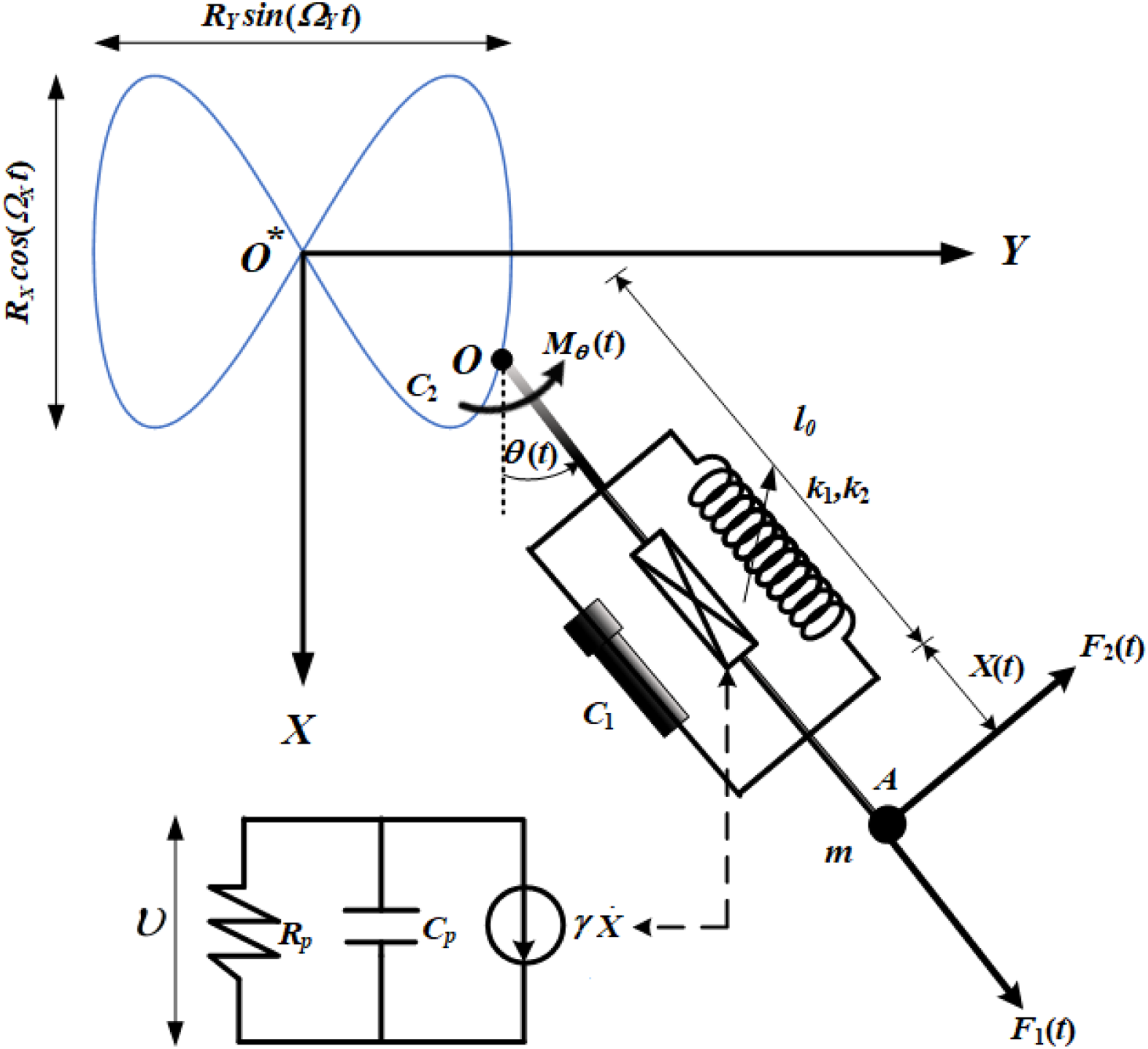
This section introduces the required investigated system, in which the EOM can be obtained in main form and the corresponding dimensionless ones, besides the piezoelectric circuit equation. Therefore, let’s have a look at the motion of a 2DOF dynamical system that includes a nonlinear SP that has a linear stiffness coefficient and a nonlinear one with coefficient , respectively. The point of suspensions is limited to travel along a Lissajous curve with angular velocity in the direction of anticlockwise direction with coordinates and , where and are known parameters.
To follow the description of the resented system, we take into account the action of two harmonic external forces, on the mass along the spring direction and in the direction of increasing the rotation angle , in addition to the moment acting at and represents the spring elongation, as seen in Figure 1. Here, and are the frequencies and amplitudes of and , respectively. Let and denote the coefficients of damping of the damping force and damping moment , respectively, is the pendulum’s normal length and is the gravity’s acceleration. The resistive load of the piezoelectric circuit will now be taken into consideration in the connection of a piezoelectric device. Let points to the linear coupling coefficient for the piezoelectric circuit, and signifies the piezoelectric capacitance.
The dynamical system with piezoelectric EH devices.
We may express the mass’s Cartesian coordinates as follows
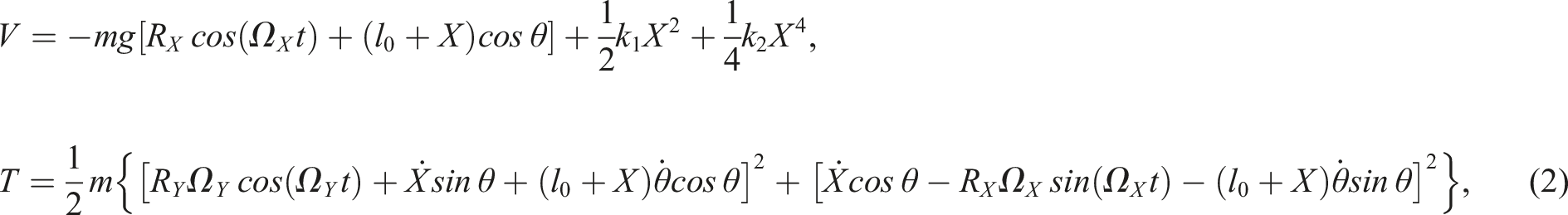
The dynamical system’s potential and kinetic energy may now be expressed as
where the differentiation over time is represented by the dot. The following second kind of Lagrange’s equations are applied to derive the main EOM for the examined system.
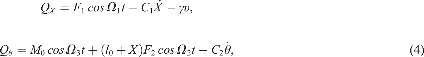
Here, expresses the Lagrangian and represents the related forces of the coordinates which have the forms
where is the voltage of the load’s resistance . Additionally, the mechanism’s equation for the circuit of piezoelectric may has the form20
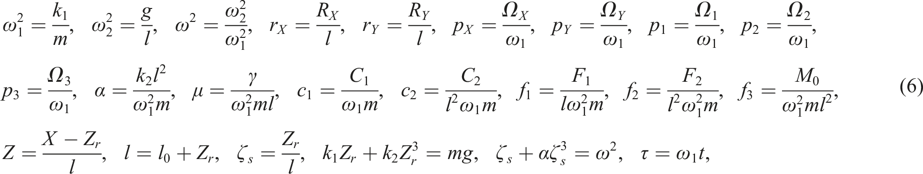
Now, let’s have a look at the following dimensionless parameters
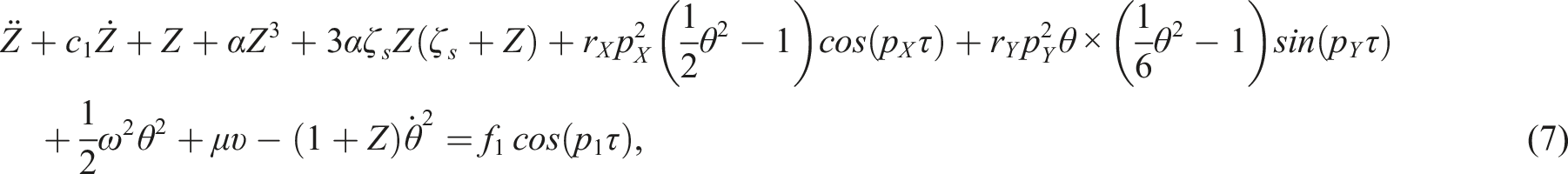
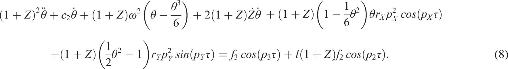
where is the spring’s static elongation. The substitution of (2), (4), and (6) into (3) produces the below governing EOM in dimensionless forms
The dimensionless mechanics equation of the piezoelectric circuit may be determined using the procedure above by substituting (6) into (5) as shown below.
The suggested approach
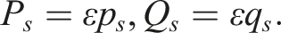
In the current section, the MST is used to obtain the asymptotic analytic solutions of the aforementioned system of equations (7)–(9). Therefore, we focus our study on the dynamical behavior of this system in a tiny region that is closed to the point of static equilibrium point.23 Then, one can express its vibrational amplitudes as follows
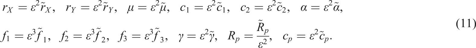
where is a small parameter. The smallness of parameters and variables was taken into consideration in accordance with
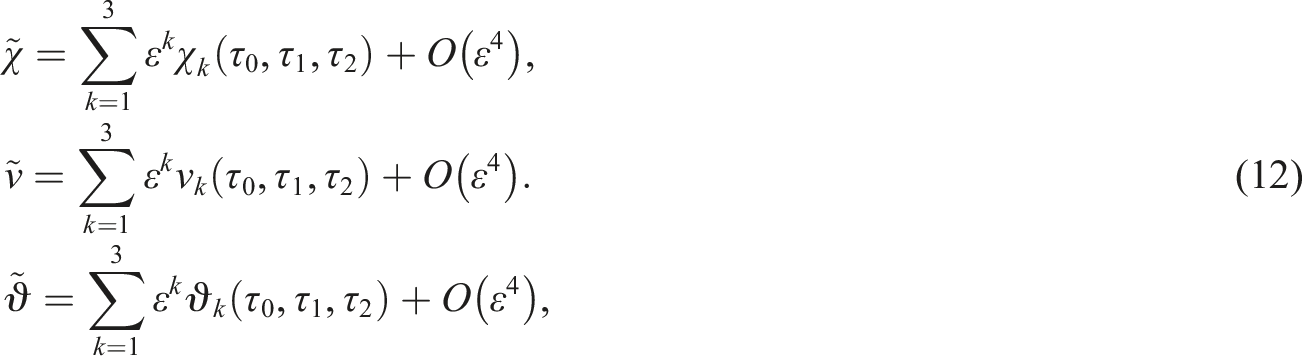
According to the MST methodology, the solutions and , can be expressed as as shown below 26
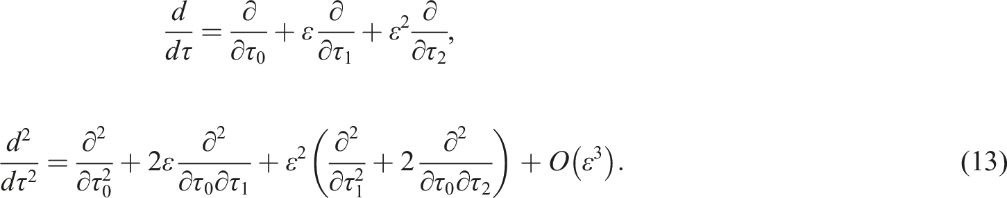
Here represent specific time scales, in which is a fast one while and are the slow ones. Now, the derivatives with regard to must be transformed to these scales. Accordingly, the use of the following operators fulfils this purpose
It is clear from these operators that terms and higher are not taken into account for their smallness. The substitution of (10)–(13) into equations (7)–(9) yields the below sets of partial differential equations that are linked to the various powers of :
(a) Order
(b) Order of
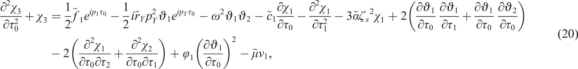
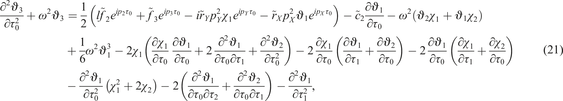
(c) Order of
Within the framework of the previous equations (14)–(22), it can be stated that they can be solved sequentially which emphasizes the significance of the solutions that are provided by the first group of equations (14)–(16). Consequently, the general solutions of equations (13)–(15) have the forms
where portray unclear, complex processes functioning at slow time scales , while indicate their complex conjugate. It is known that the secular terms can be produced by substituting the previous solutions (23)–(25) into the higher order partial differential equations (17)–(19). The following conditions can be used to eliminate them
Consequently, the subsequent second-order solutions are as follows
where indicates the conjugations of the previous expressions. Similar to the earlier case, the canceling of the secular terms requested that depended on . Therefore, canceling these terms produces the following conditions
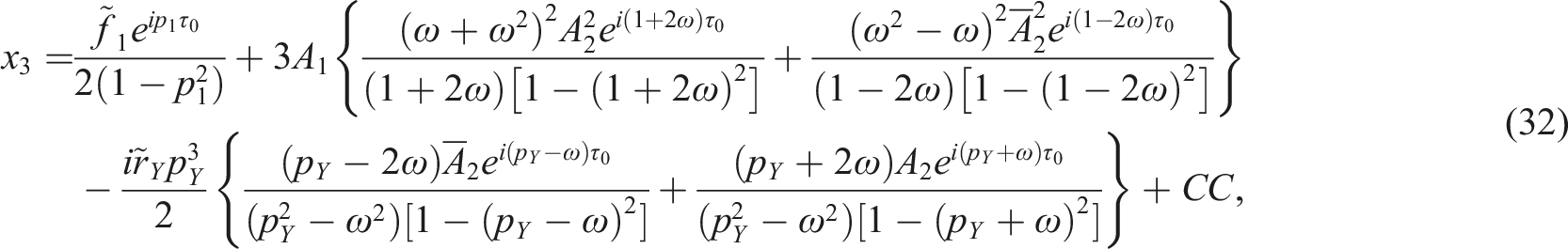
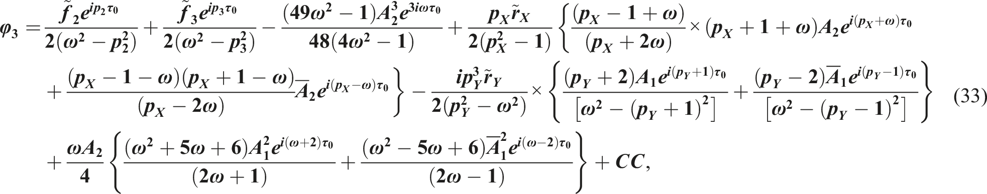
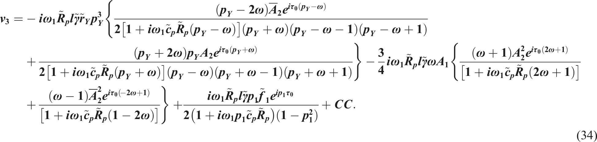
Finally, we can get the below third-order solutions
Resonance categorization and modulation equations
This section’s goals are to categorize the resonance cases, address with one potential case, and obtain the modulation equations. When the denominators in the second and third order solutions disappear, these situations may appears.41 Consequently, the following possibilities are obtained
1- The case of primary external resonance is obtained at
2- The case of internal resonance will be satisfied at
When one of the preceding prerequisites for resonance is satisfied, the examined system will behave in a very complicated manner. It’s crucial to note that even if the oscillations are far from resonance, the solutions produced are still appropriate. We’ll now look into the first case in greater depth, in which two of them occurred simultaneously, that is, . Then, one can consider the detuning parameters that help achieve this aim, which express the nearness of and to and , respectively. Therefore, one writes
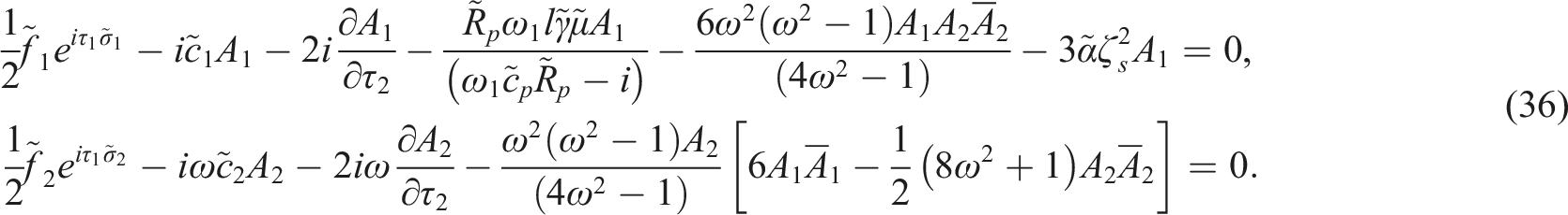
where . Detuning parameters are seen as a distance from the vibrations and the strict resonance. Eliminating secular terms makes it possible to acquire the criteria of solvability. As a consequence, the next equations estimate that the necessary conditions are fulfilled
The established requirements of solvability (26) and (36) constitute four nonlinear partial differential equations regarding to that rely on the slow time scale . As a result, we may consider the polar form of these functions as:
Since the functions don’t depend on the scales and , it is possible to simplify the first-order derivative operator as follows
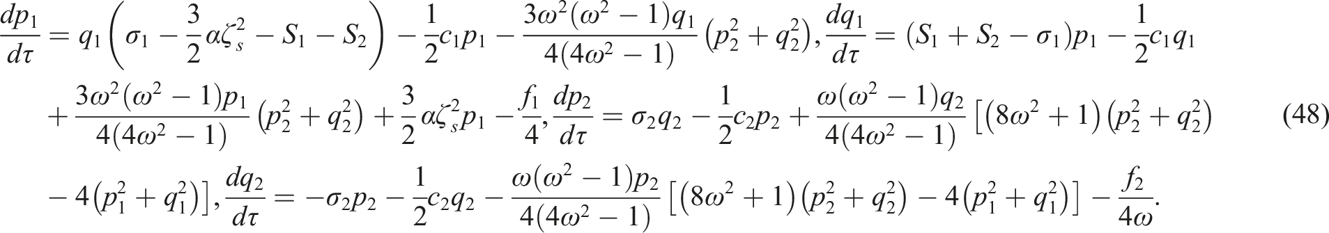
Referring to (38), the criteria of solvability (36) may be transformed into ordinary differential equations by using next modified phases
Substituting (37)–(39) into (36) and separating the real and imaginary portions, one obtains the below required system
Here, and .
Numerical results
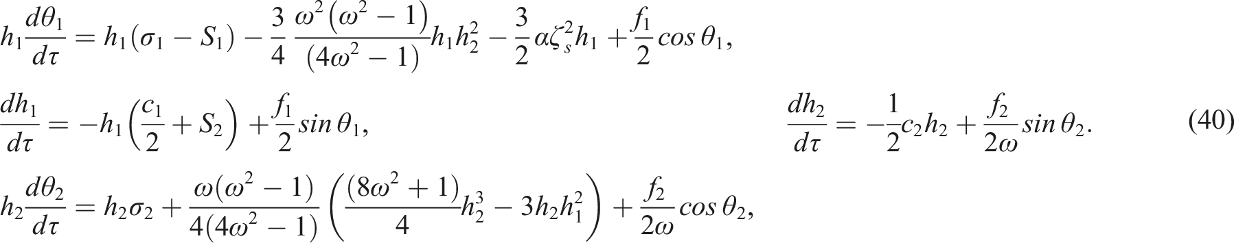
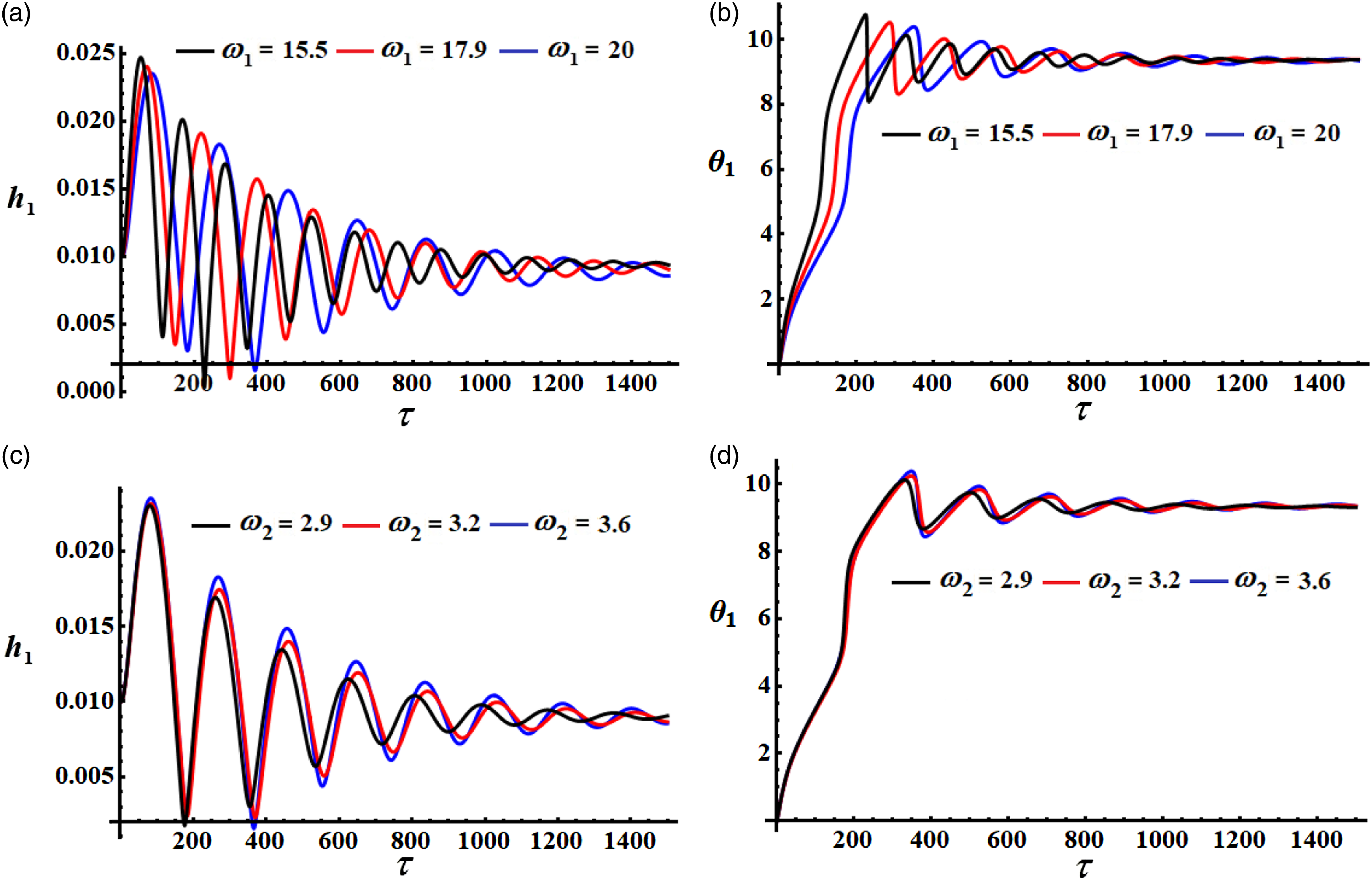
This section is devoted to examining the numerical solutions of the aforementioned system (40) using the Runge–Kutta method from fourth-order with the help of Wolfram Mathematica 13.2. It must be mentioned that these equations cannot be solved analytically to obtain the amplitudes and the modified phases and . Therefore, the following listed initial circumstances are taken into account In Figures 2 and 3, and are displayed to show the temporal histories of the amplitudes and the adjusted phases . It has taken into account the below values of the used parameters for the sketched curves:
The amplitude and the modified phase as a function of the dimensionless time parameter at: (a), (b) , and (c), (d) .
The amplitude and the modified phase as a function of the dimensionless time parameter at: (a), (b) and (c), (d) .
The calculations for these figures were performed for various values of and as indicated, respectively, in portions [(a), (b)] and [(c), (d)]. As time goes on, the oscillations of the waves described by the amplitude have decaying behaviors, as shown in Figure 2(a) and (c). On the other side, the behaviors of the waves increase to certain values, and then they behave in a stationary manner, as seen in Figure 3(a) and (c). Furthermore, the variance of the typically displays a stable behavior once it reaches a certain value over time, as seen in Figures 2(b) and (d) and 3 (b) and (d). Based on these simulations, one can conclude that and exhibit stable behaviors.
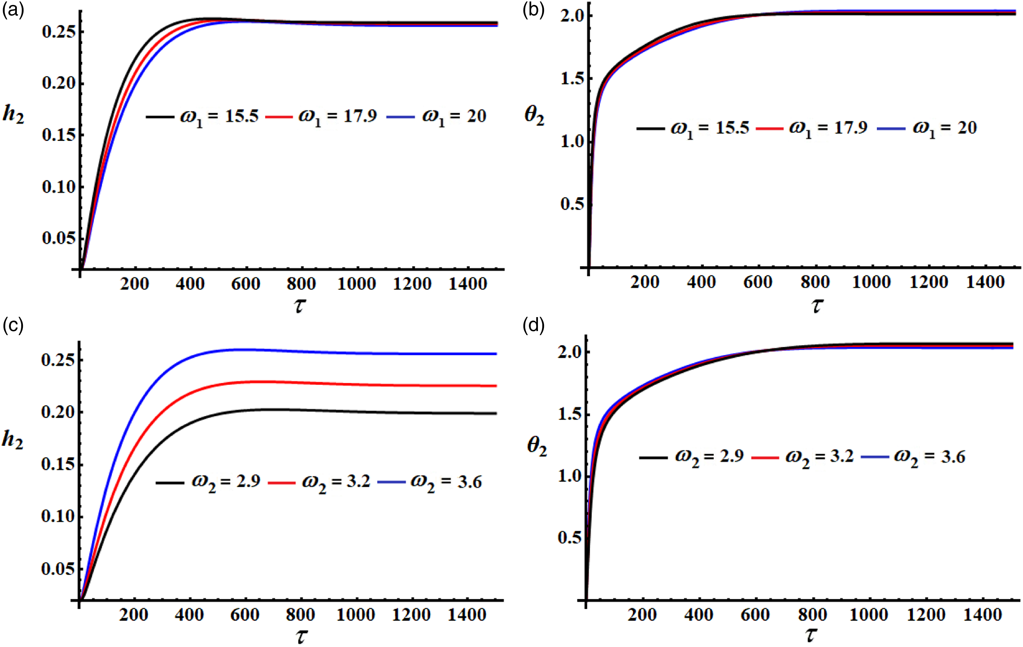
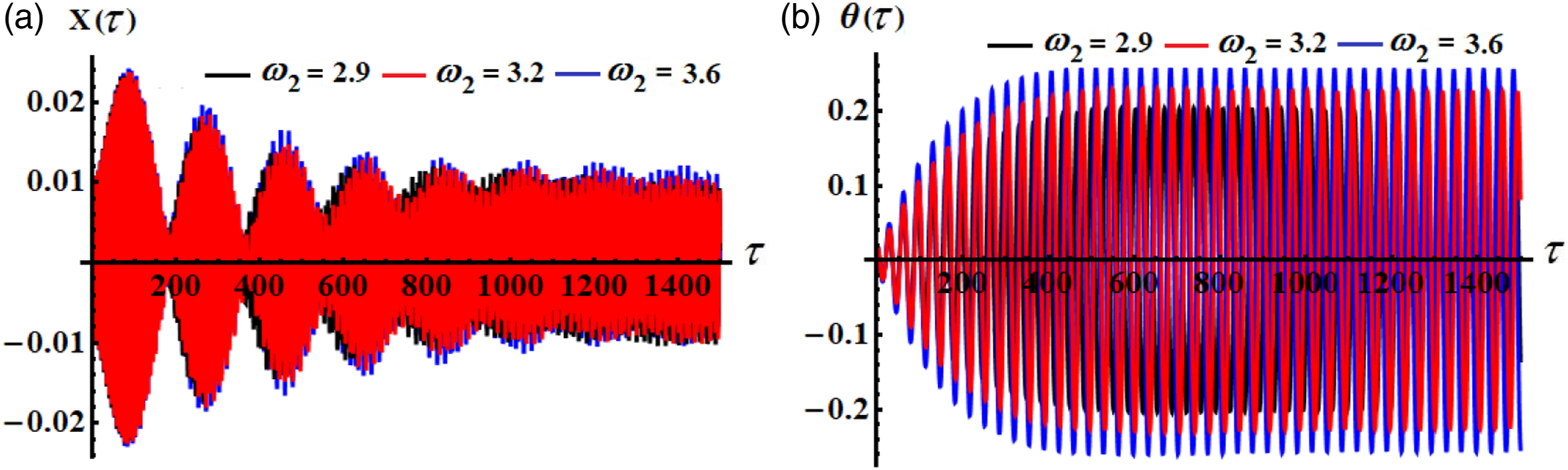
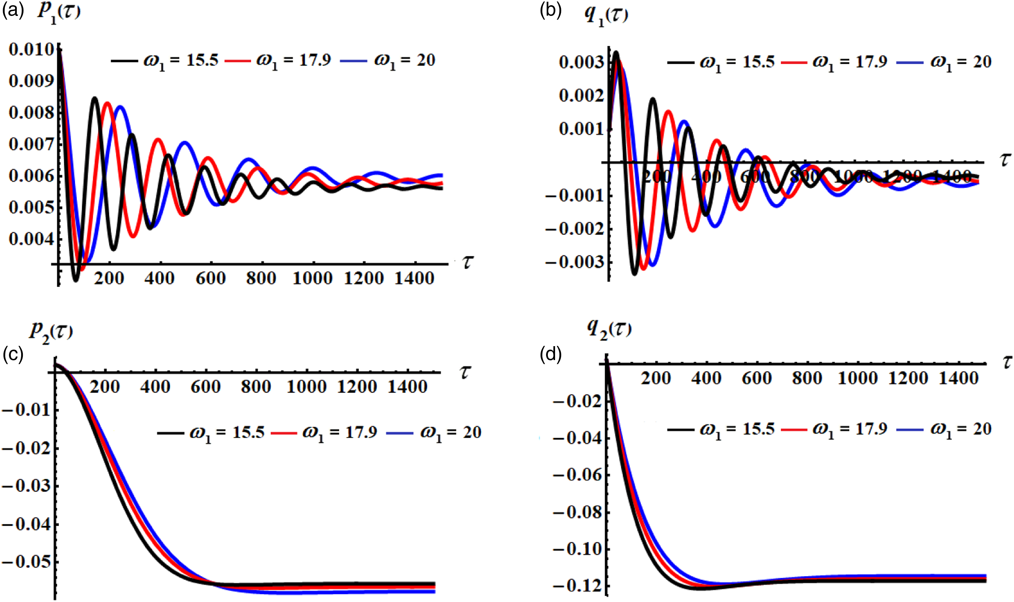
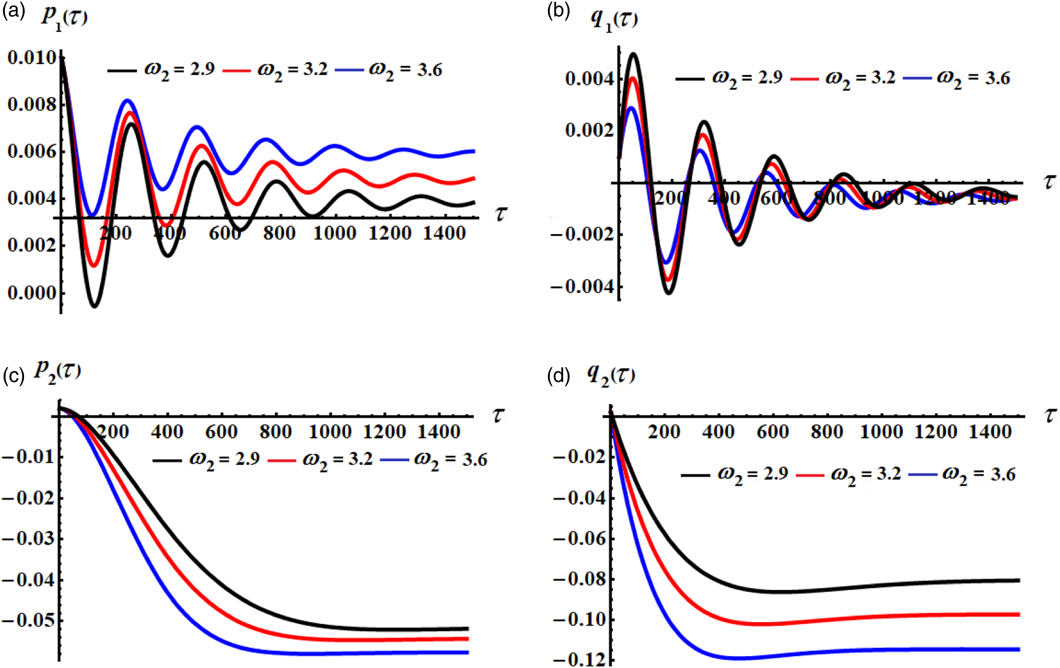
Figures 4 and 5 depict the time histories of the found approximative solutions and , up to the third degree of . These graphs are created using the previously utilized data at various settings . We may infer from the portrayed curves in these plots that the behavior of the solution as a function of the dimensionless time take the form of decaying waves, which are represented by wave packets with decreasing amplitudes until they reach a certain value, and then they have the form of stationary flow, see drawn in Figures 4(a) and 5(a). However, the amplitudes of waves illustrating the time behavior of the solution increase to specified values, then they have stationary till the end of the investigated time interval, as displayed in Figures 4(b) and 5(b).
Time history of the asymptotic solutions and when the frequency has various values.
Time history of asymptotic solutions and when the frequency has various values.
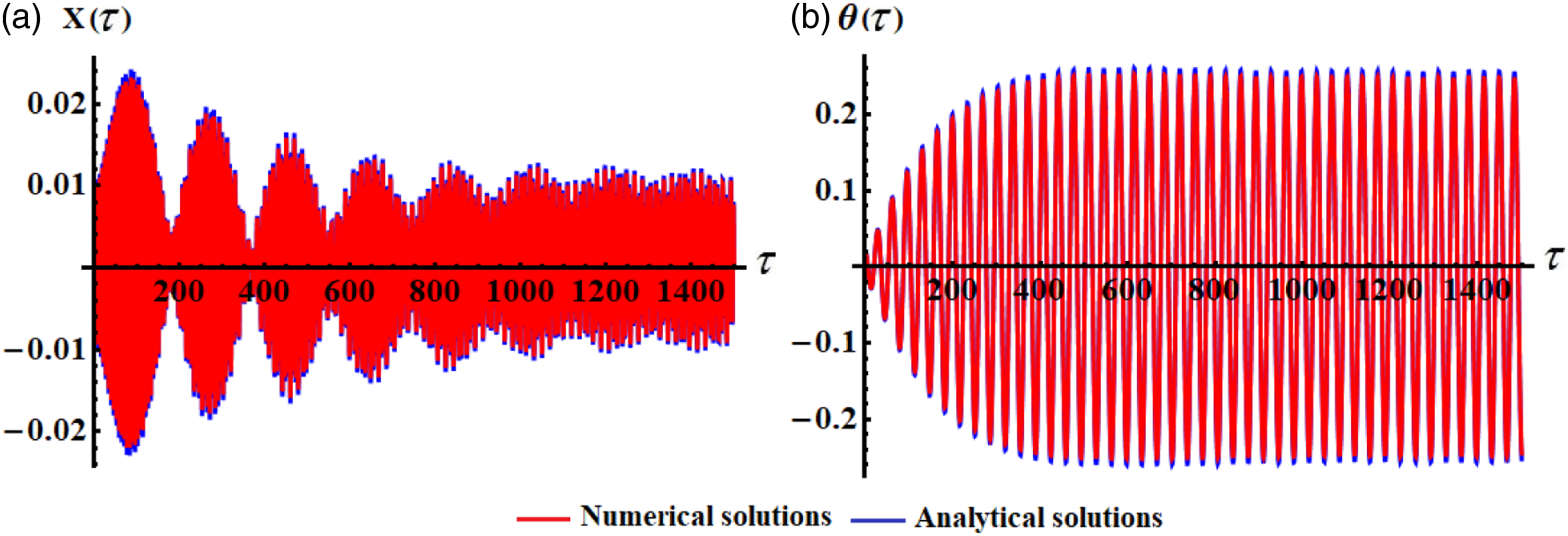
The analytic solutions and the numerical ones of the original EOM are plotted graphically, as seen in Figure 6. A deeper examination of this figure reveals excellent consistency between the two solutions, which is an indication of the approximations’ high accuracy.
Comparison between the numerical solutions and the analytical ones at and when and .
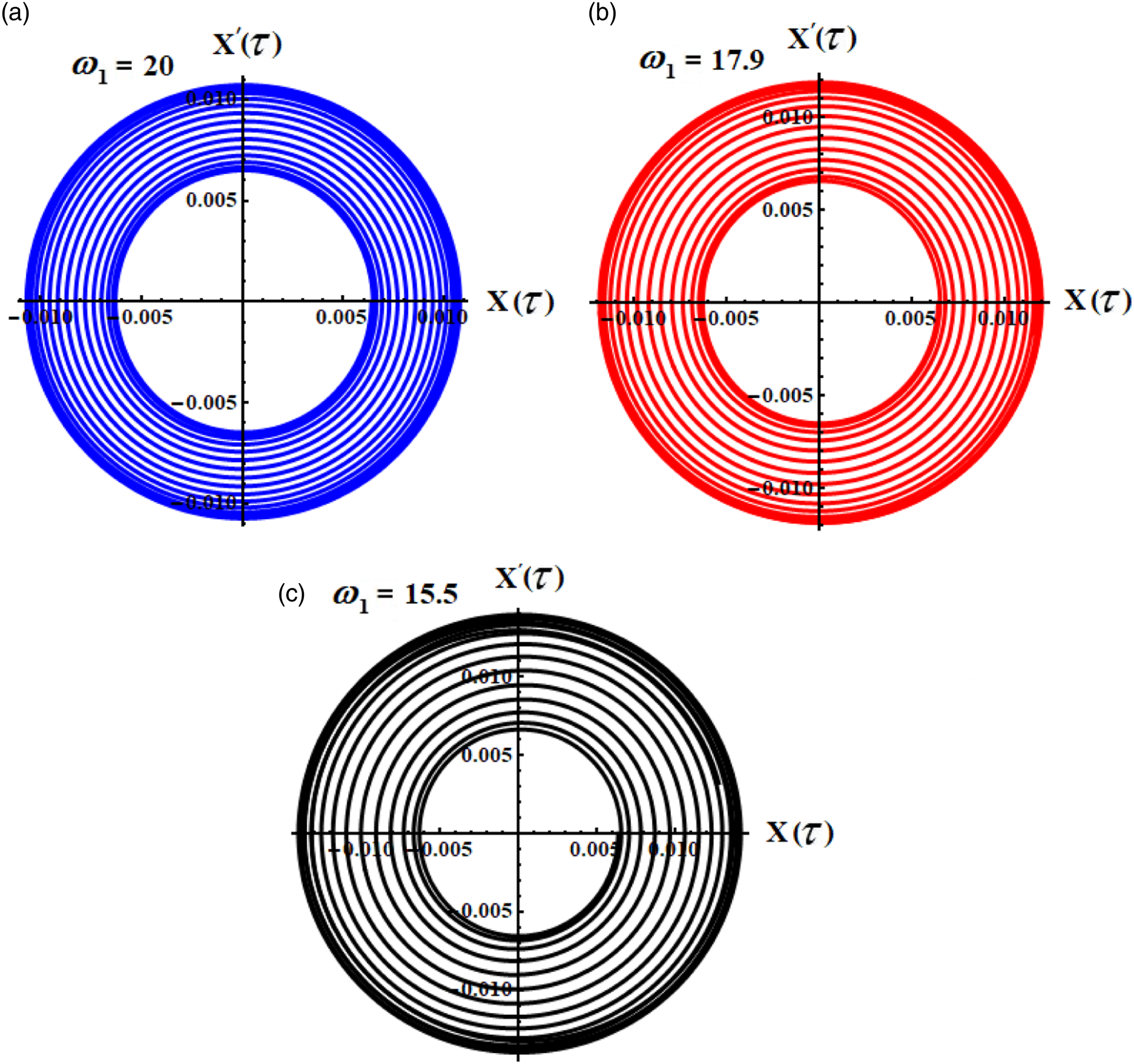
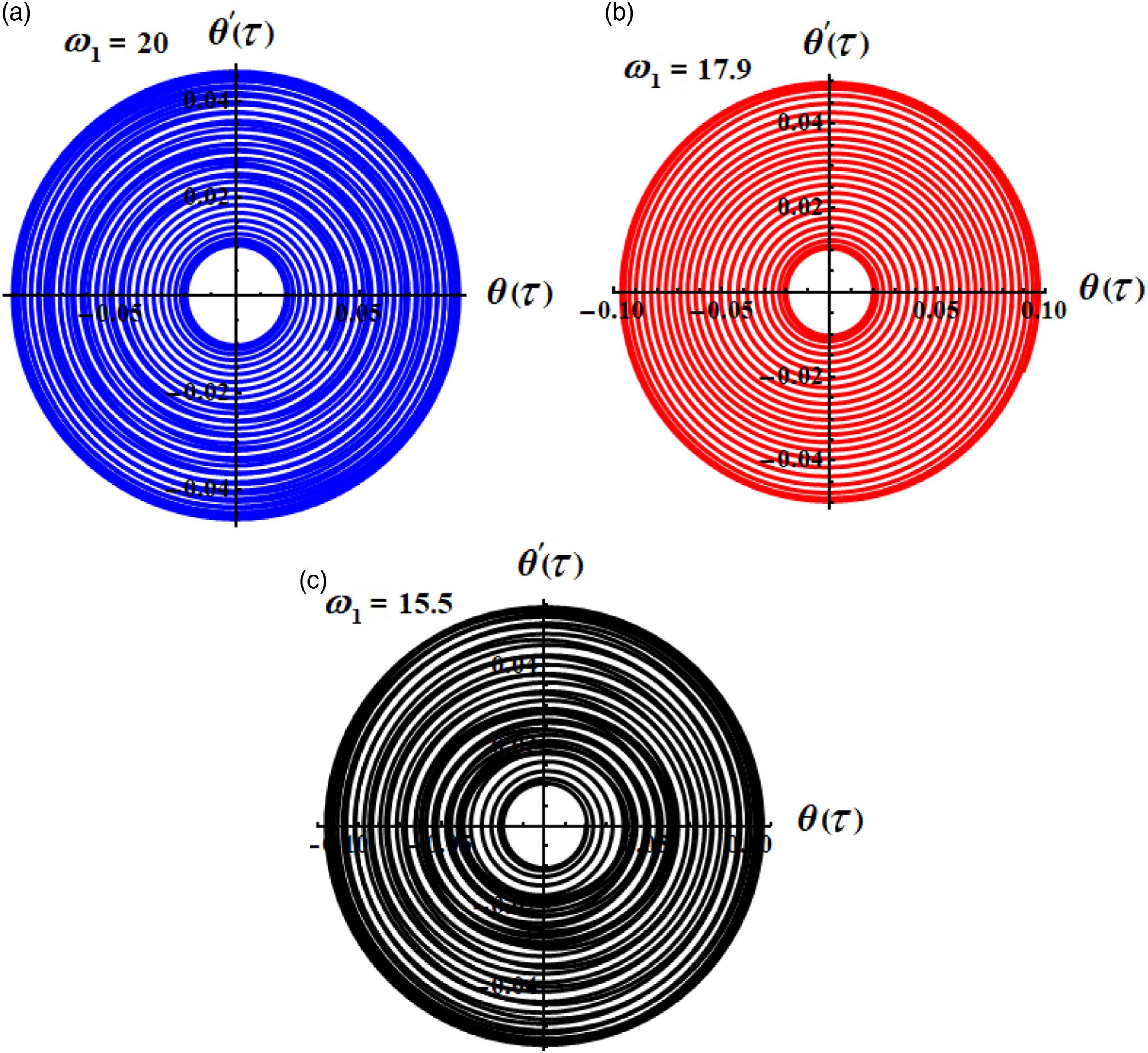
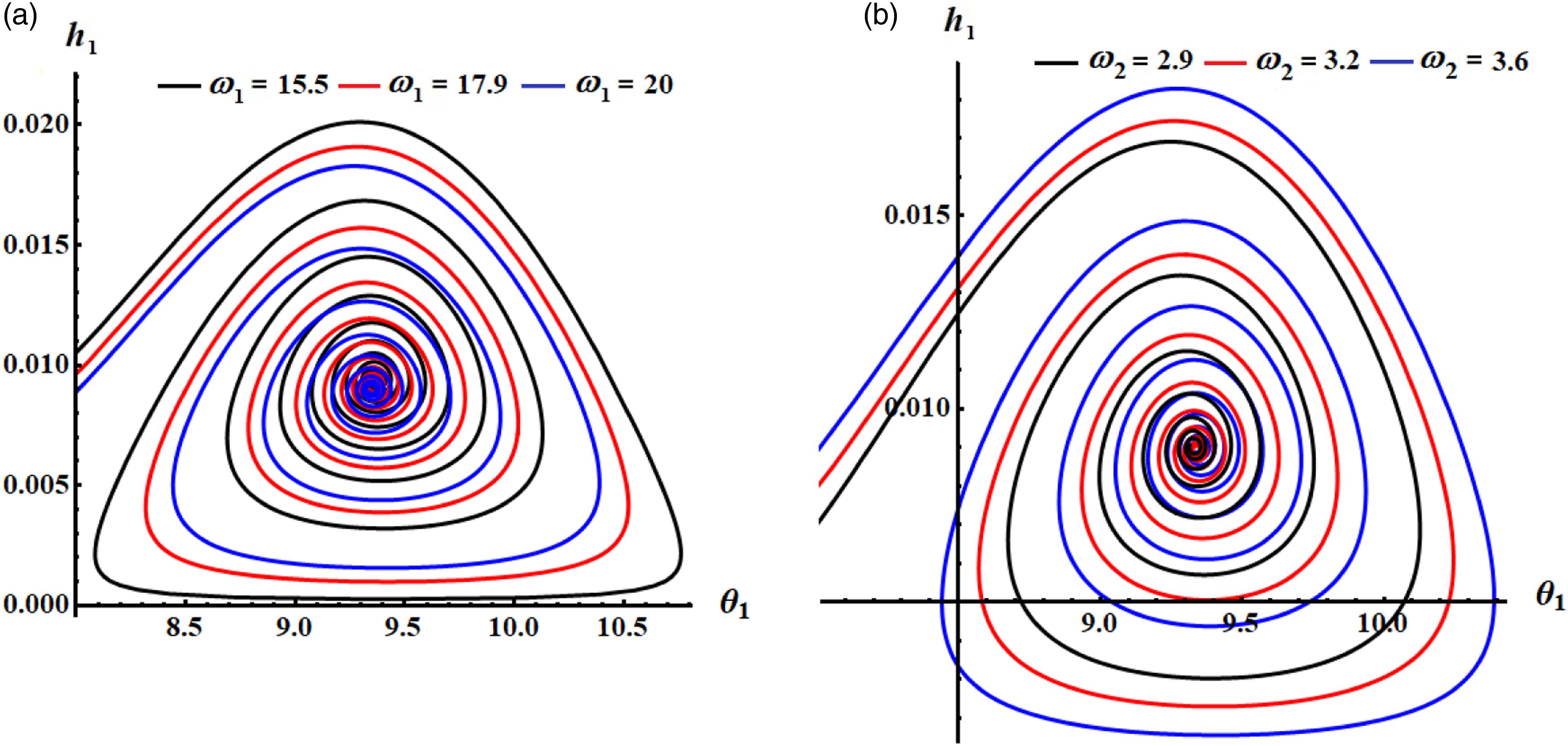
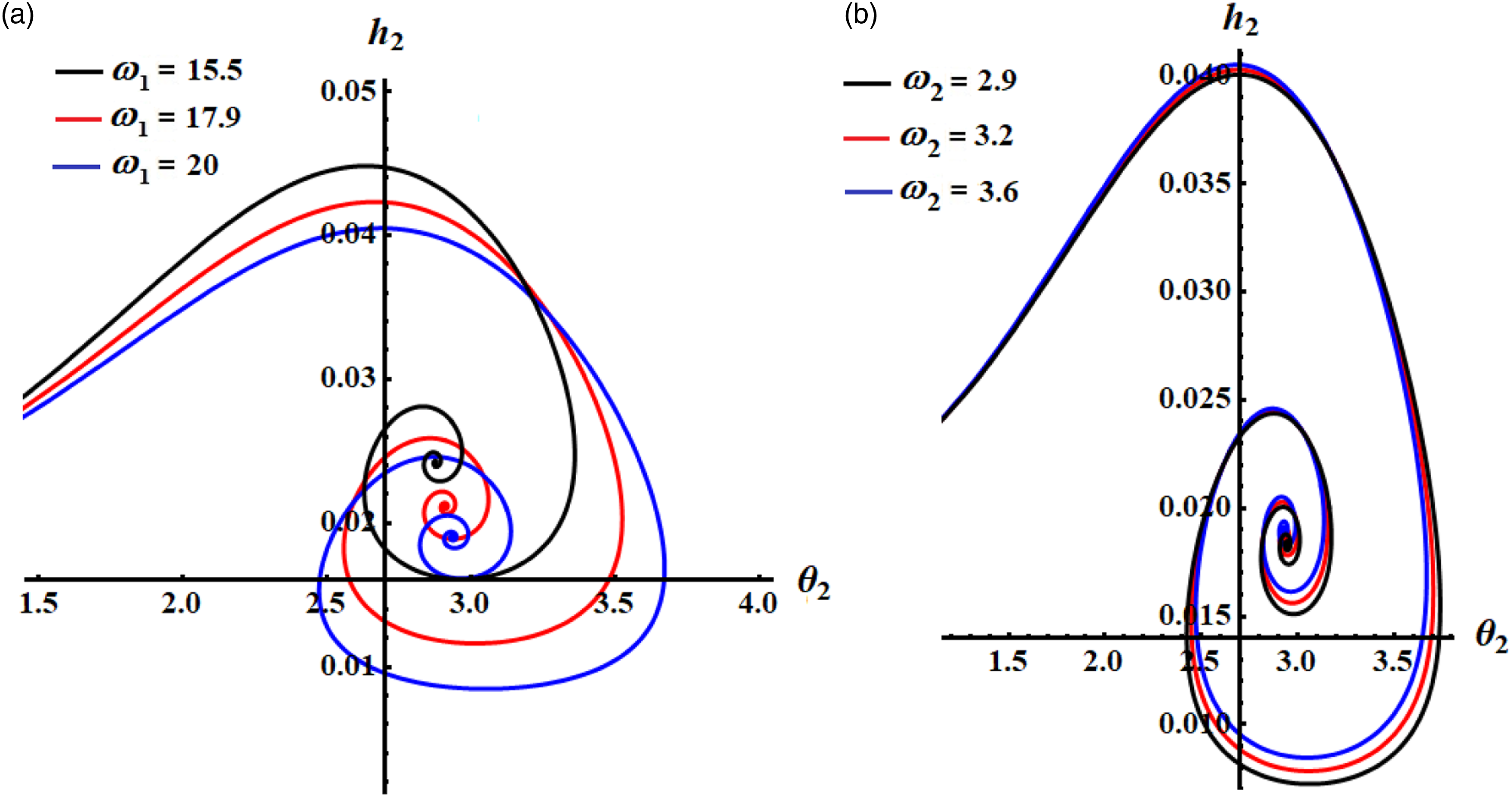
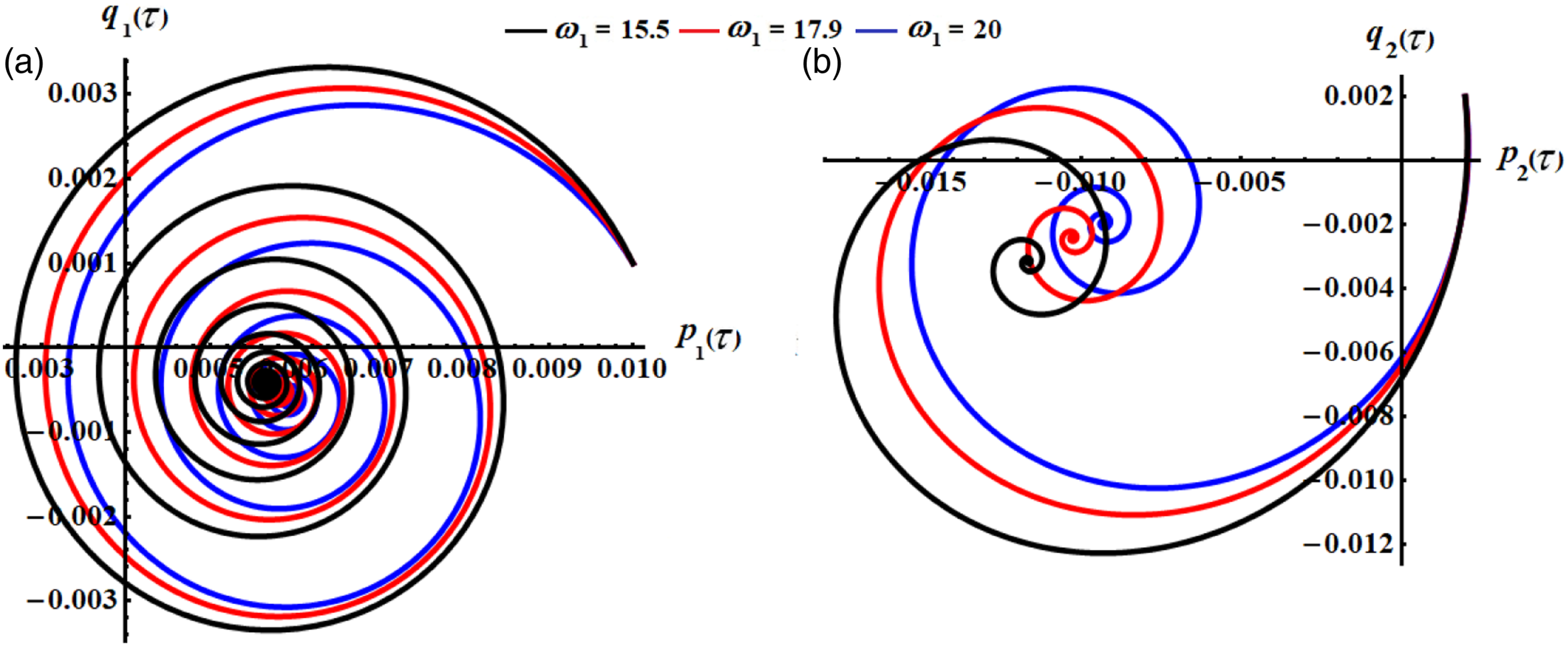
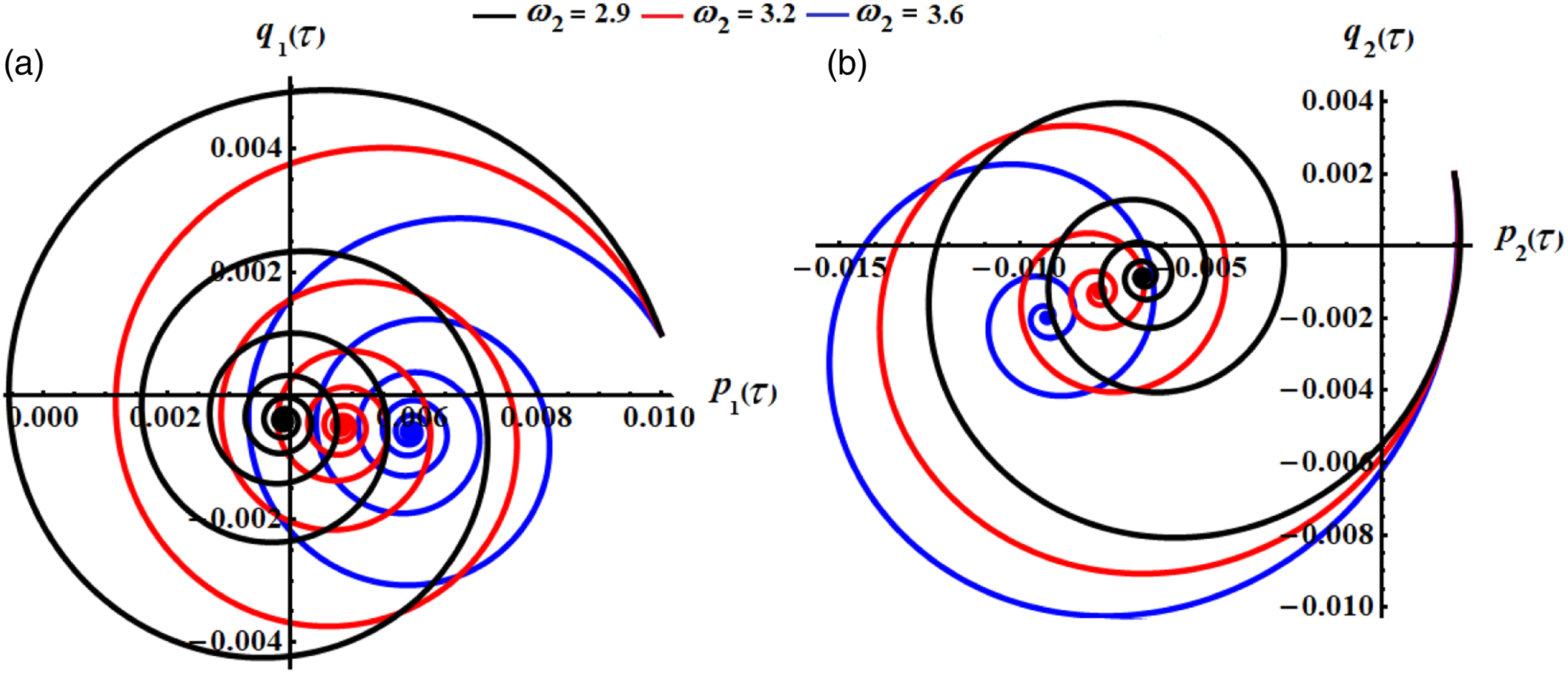
The graphs of phase plane for the represented solutions in Figures 5 and 6 have been displayed in Figures 7 and 8. As may be seen from the drawn curves in the planes and that they have directed spiral paths into only a certain point, which indicates their stable behavior.
Phase portrait in the plane at different values of the frequency .
Phase portrait in the plane at different values of the frequency .
To continue the examination of the stability of the studied system, the relationships between the and the have been portrayed in Figures 9 and 10 according to the numerical outcomes of the system of equation (40), which is considered one of the best ways to clarify the behavior of the system. It is observed that all curves take the form of spiral trajectories towards one point, which indicates that this system has stable behavior during the examined time interval.
The phase plane at the mentioned values of the frequencies and .
The phase plane at the aforementioned values of the frequencies and .
Stable-state approaches
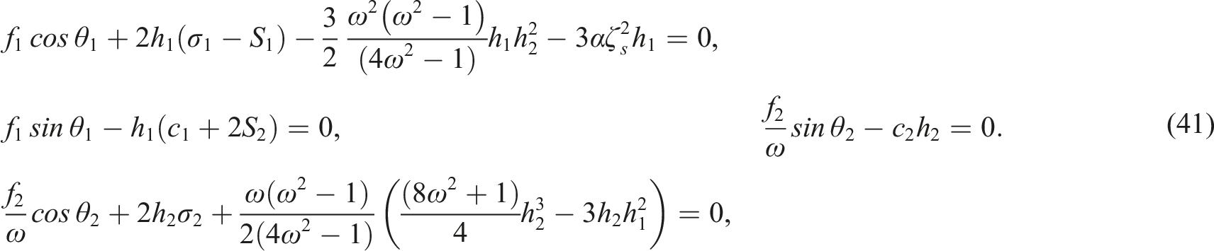
The examination of the solutions for the studied dynamical system’s steady-state situation is the main topic of this section. This scenario is where the solutions would appear when the transitory processes cease to exist. In the present scenario, we take into account the zero value of .27 Therefore, by using the system of equation (40), we may generate the following form of algebraic equations:
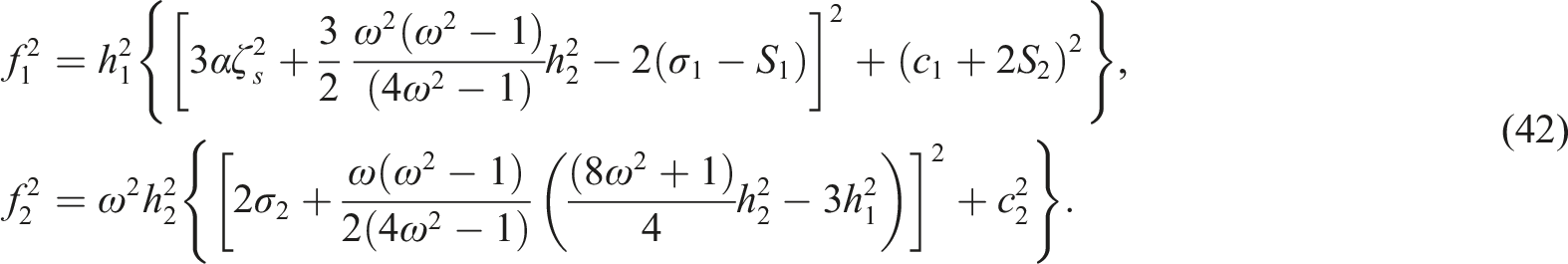
According to an examination of the previous system (41), the below frequency response functions are produced when the altered phases are removed from its equations.
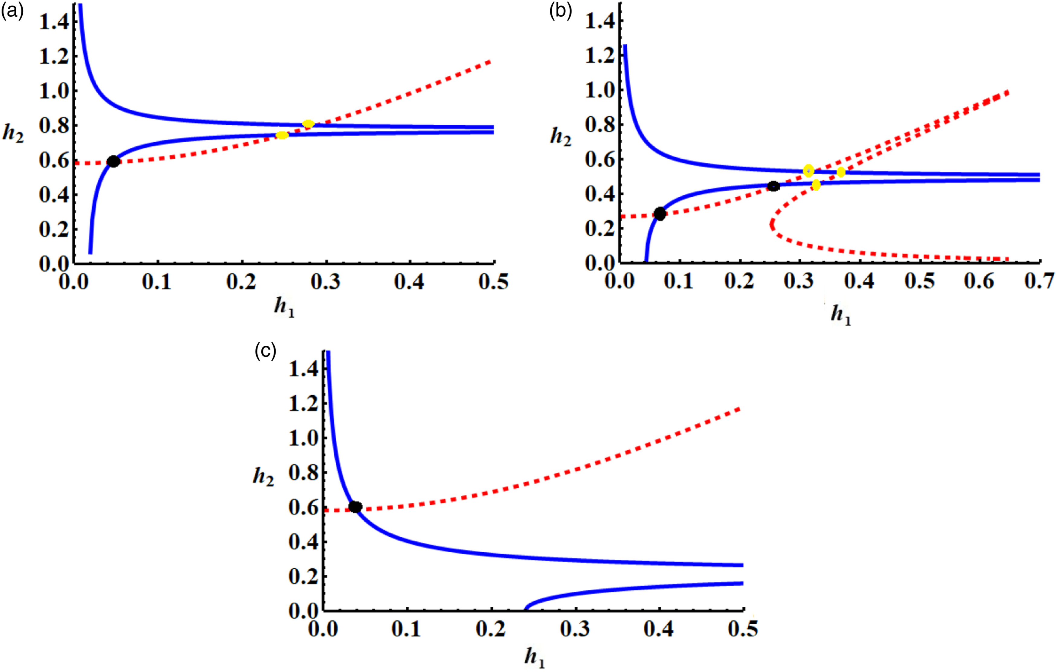
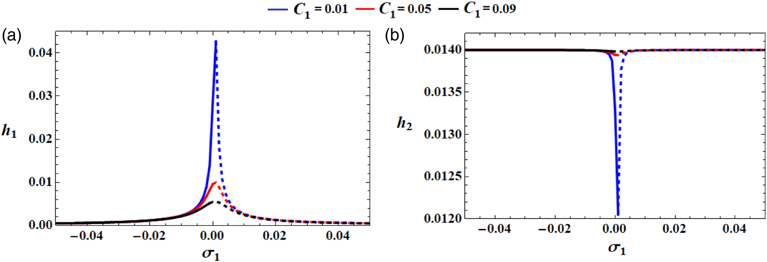
It is crucial to remember that all potential steady-state solutions may be represented for the amplitudes at and , within the context of system (42), as depicted in Figure 11, in which it has been calculated for certain data of . The blue and dashed red curves show, respectively, the roots of the first and second equations of system (42). In other words, these curves show where the roots of these equations are located, and the spots where the two curves cross reflect the fixed points that are equivalent to the solutions at the steady-state scenario. These points provide an irrefutable formula for determining the axial amplitudes and regulating vibration in the steady-state. Furthermore, steady-state oscillations could be either stable or unstable. Small black circles are used to denote the stable fixed points, whereas small yellow ones are provided to denote the unstable case of fixed points.
We are going to examine the dynamical system’s behavior in a location close to the fixed points for further investigation of its stability. For this goal, we take into account very slight changes to the amplitudes and phases as follows.
where and indicate the steady-state solutions, while and signify the minor perturbations in comparison to and . After linearization, we may obtain the next system according to the substitution of (43) into (40).
Solution at the steady-state scenario: (a) three fixed points when , (b) five fixed points when and (c) one fixed point when .
We may express the solutions of this system as in a form of linear combination of where are constants and is the unknown perturbation’s eigenvalue, respectively, that predicated on the tiny of the perturbations functions and . In light of the above, the fixed points in (44) are stable asymptotically when the real portions for the roots of the next characteristic equation are negative.
According to Routh– Hurwitz criteria,42 the following conditions must be met in order for fixed points to be stable:
Examination of stability
This section’s goal is to investigate the examined model’s nonlinear stability using the approach of nonlinear stability.43 On the basis of the foregoing, the dynamical motion is impacted by the external harmonic forces and moment . Furthermore, to simulate the system of nonlinear equation (40), the stability conditions are used. It was discovered that a number of stability criteria factors, including frequency , damping coefficients , and detuning parameters , significantly contribute to instability. To display the associated diagrams of the system’s stability, suitable regulations are used with a variety of system (40) parameters. The amplitudes for the waves describing the solutions time histories are shown in separate parametric regions, and their characteristics are graphed throughout the phase plane’s trajectories. Moreover, the potential fixed points have been plotted. Figures 12–20 examine how these points vary depending on the detuning parameters .
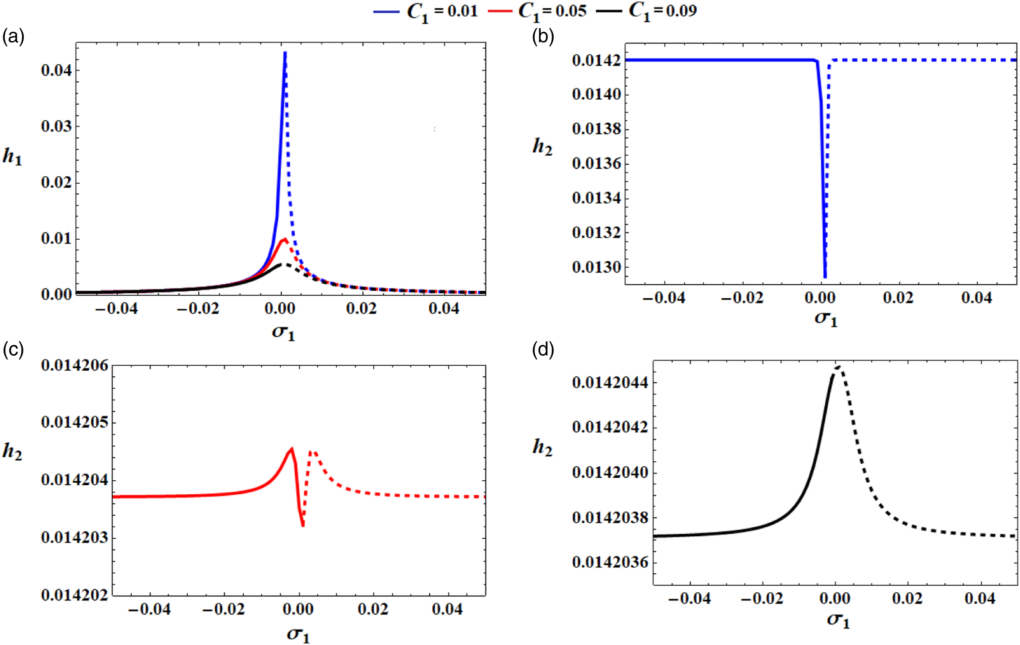
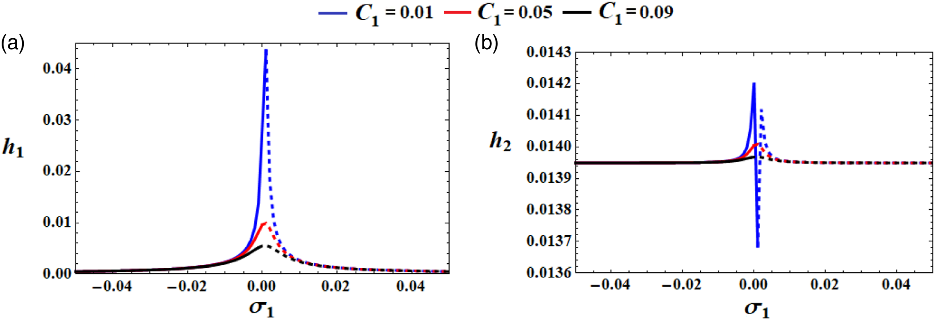
The FRC of the amplitudes at different values of at and .
The FRC of the amplitudes at different values of when and .
The FRC of the amplitudes at different values of when and .
The FRC of the amplitudes at different values of when and .
The FRC of the amplitudes at and when has distinct values.
The FRC of the amplitudes at and when has distinct values.
The FRC of the amplitudes at and when varies.
The FRC of the adjusted amplitudes at and when varies.
The FRC of the modified amplitudes at and when varies.
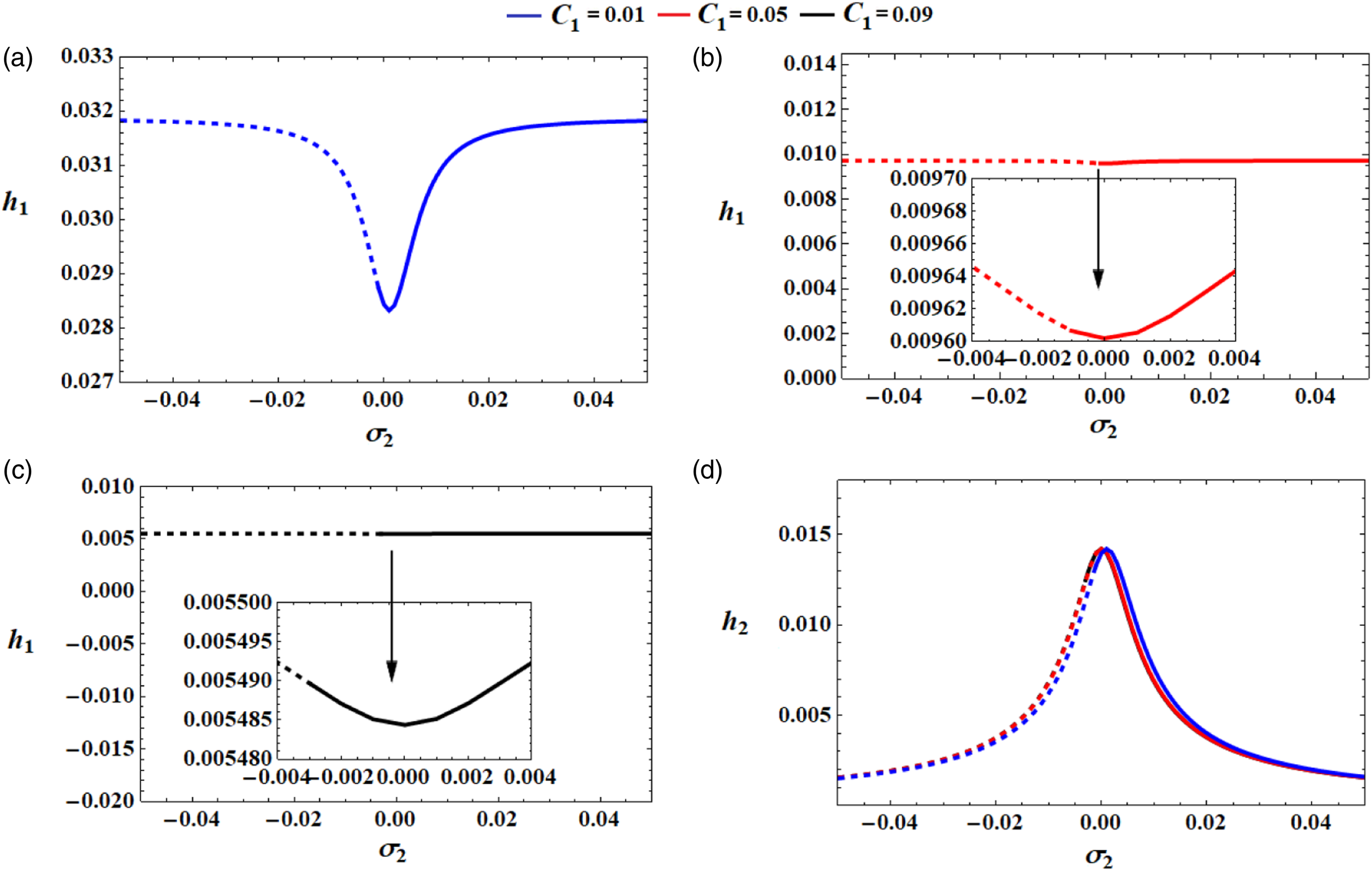
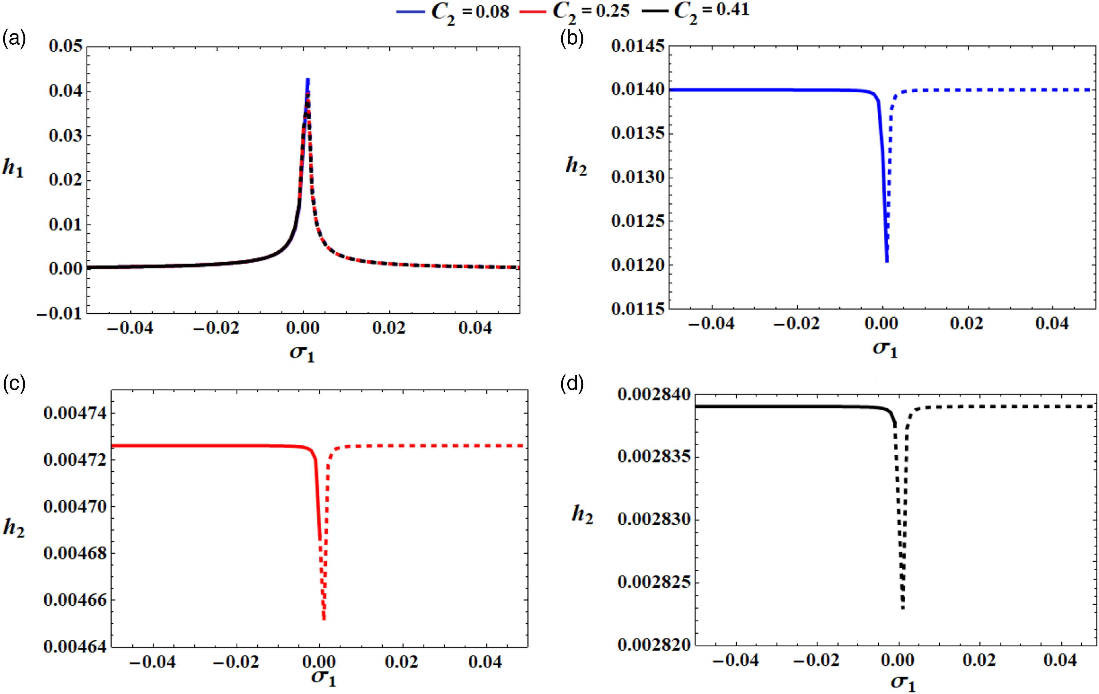
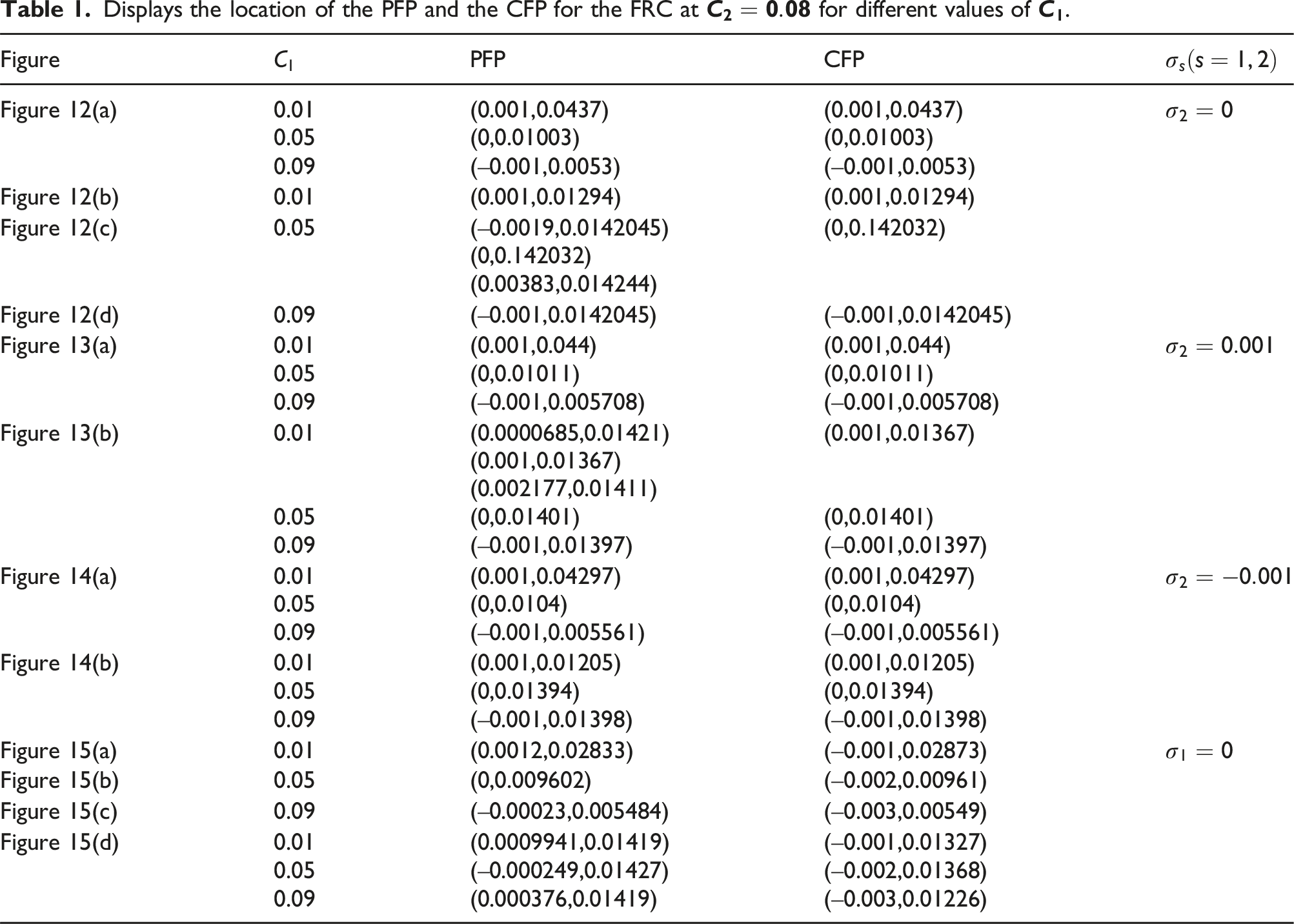
The displayed curves in Figure 12 are calculated at the zero value of and , in addition to the various values of . It must be noted that the dashed and solid curves are used to depict the unstable and stable fixed points. A more detailed examination for the parts of this figure shows that the amplitude vary with the change of the values of , as indicated in Figure 12(a), while the variation of according to the values of the same parameter seems to be slightly as observed in Figure 12(c)–(e). Moreover, the ranges containing the zones of stability and instability are and , respectively, when for the blue color. On the other hand, when and , the stability and instability areas are found at the ranges , and , , respectively, for the red and black curves. This graph has eight peak fixed points (PFP) and six critical fixed points (CFP). The distribution of these points covered all portions of Figure 12 and their locations are stated in Table 1.
Displays the location of the PFP and the CFP for the FRC at for different values of .
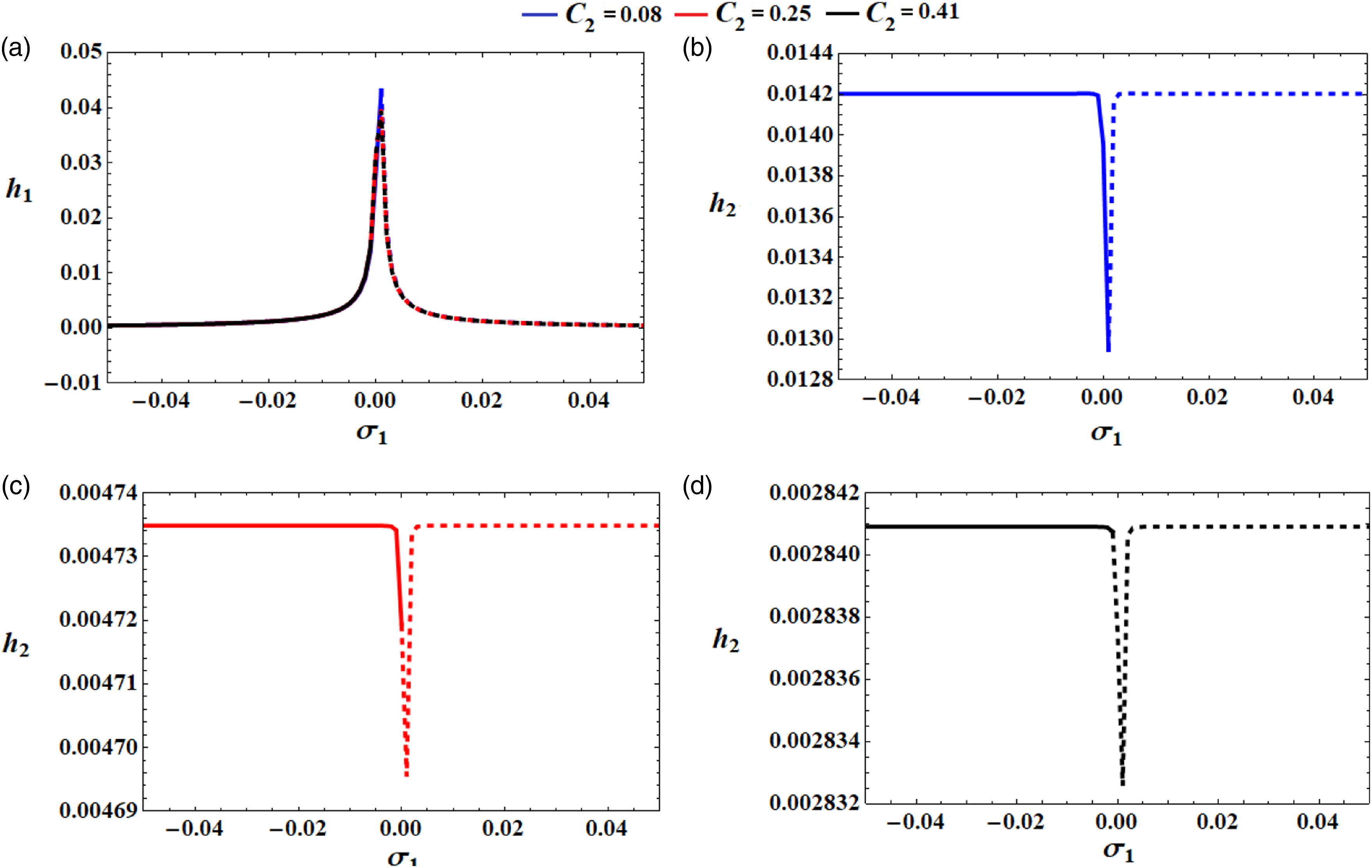
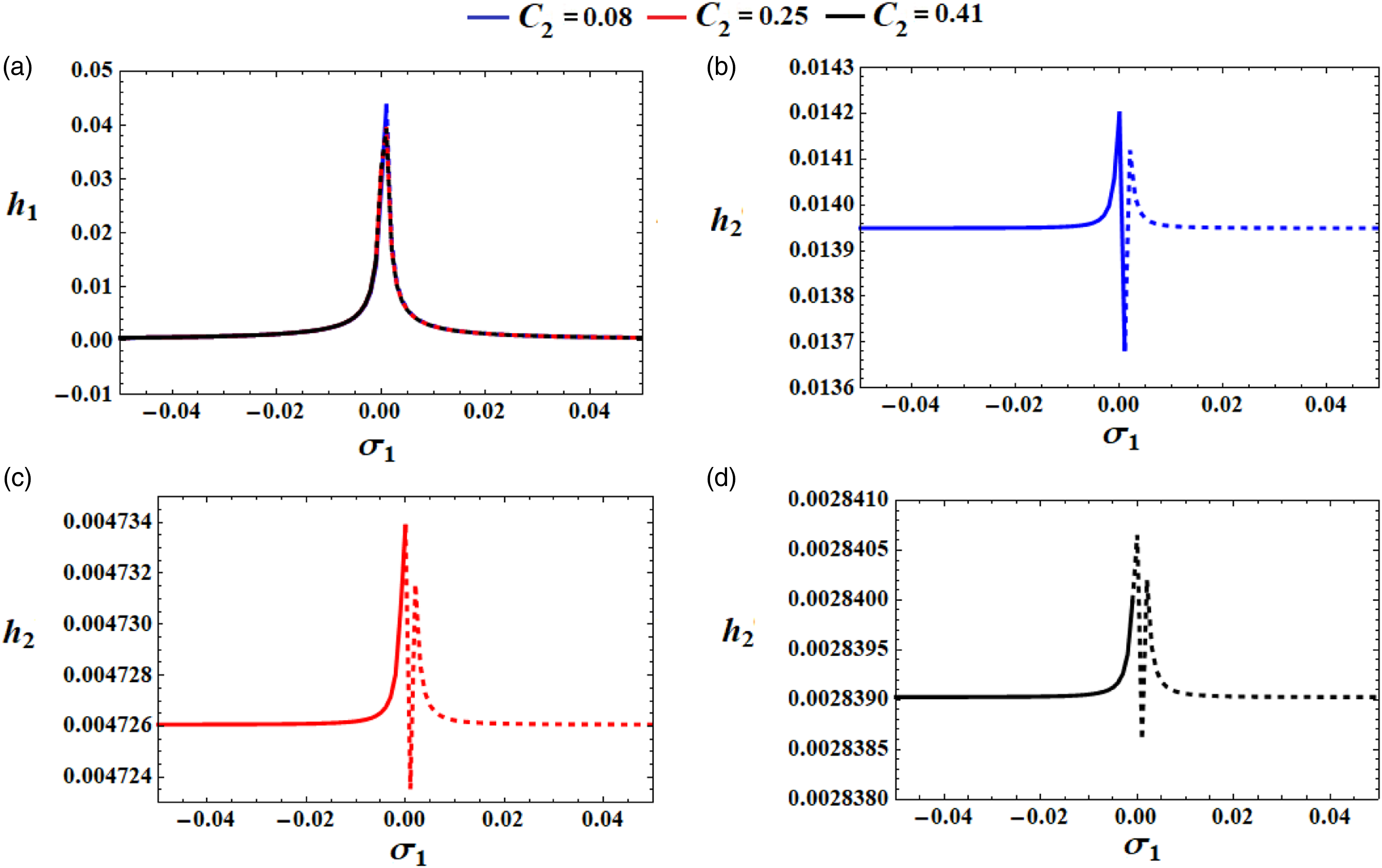
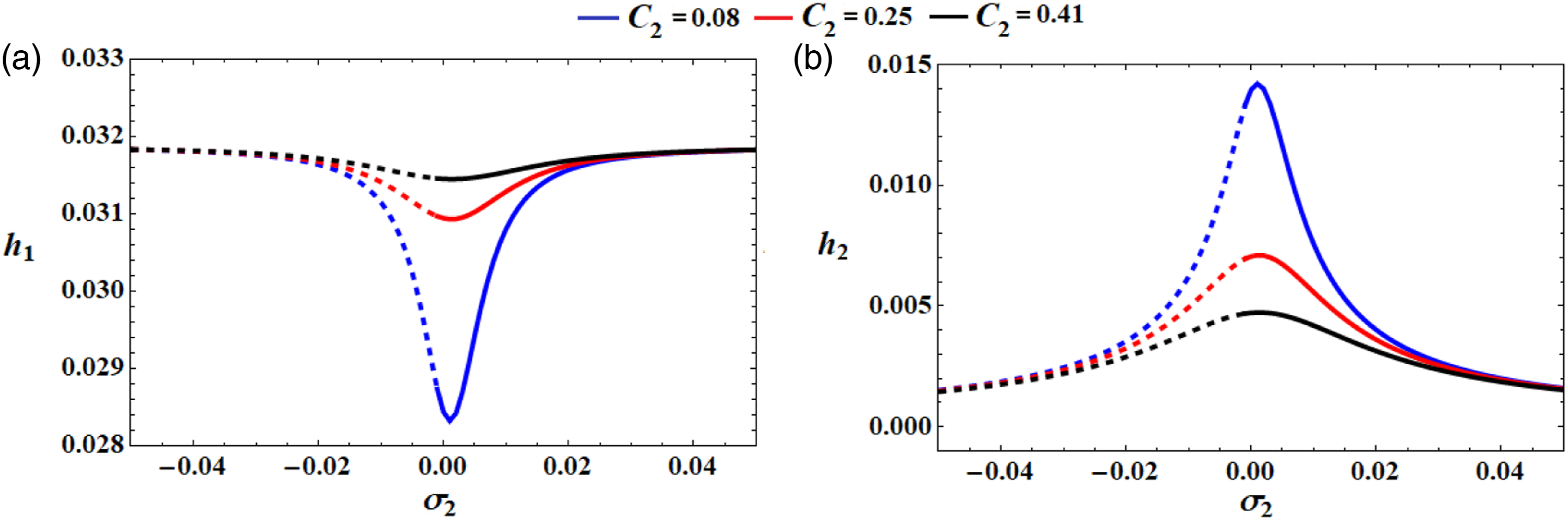
Moreover, Figures 13 and 14 show the FRC for both and at and , respectively, with the same values of and . These curves have the same areas of stability and instability of Figure 12. The good impact for various values of when on the behavior of has been described by the plotted curves in Figure 15 when and . It observed that at and , the instability and stability regions are and , respectively, with blue, red, and black colors. The observed PFP and CFP of Figures 13–15 are determined, as mentioned in Table 1. Altering the damping factor produces the behavior of the FRC for the system (4). These variations are drawn in Figures 16–18 at and , respectively. The stability and instability areas are and , respectively, for the blue, red and black curves.
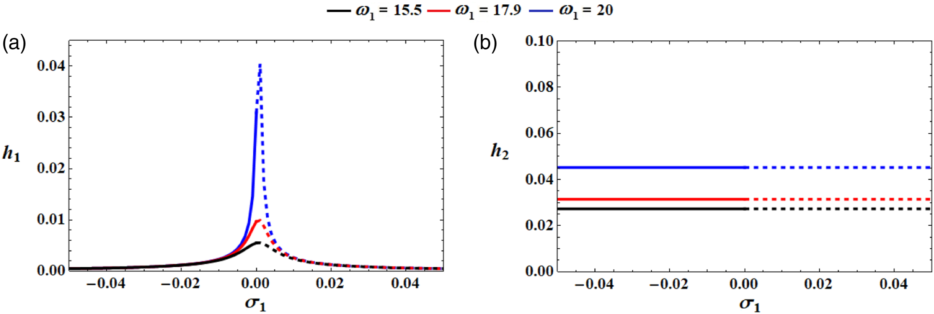
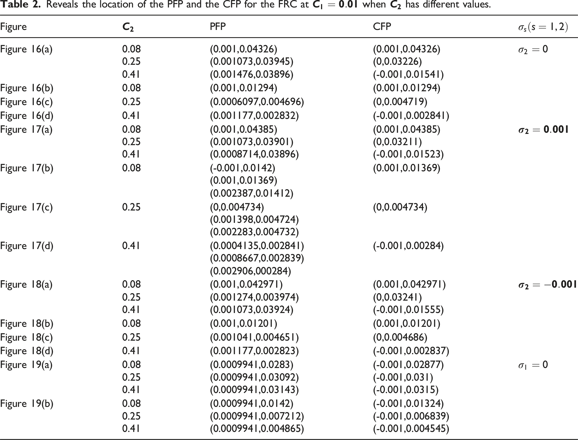
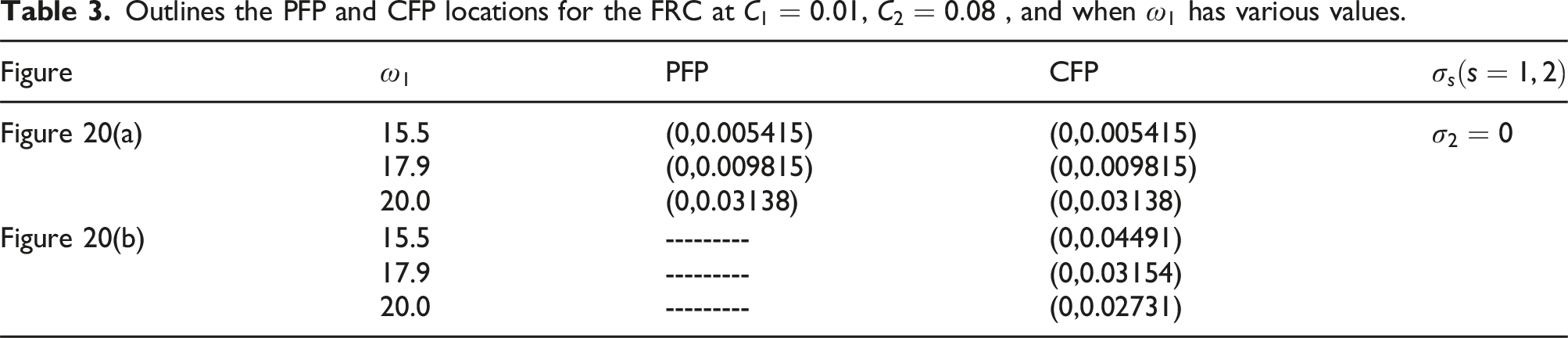
The graphed curves in Figure 19 shows and when and , while the drawn ones in Figure 20 presents and at besides the different values of the frequency . It is noted that the stable and unstable regions for the plotted curves in Figures 19 and 20 are and , respectively. The position of gained PFP and CFP for Figures 16–20 are determined, in Tables 2 and 3, respectively.
Reveals the location of the PFP and the CFP for the FRC at when has different values.
Now, we will explore the stability of the nonlinear amplitudes of system (40) and demonstrate the characteristics of the nonlinear analysis. Consequently, let’s think about the following transformations 44.
where
Making use of (40) and (47), then isolating the real imaginary terms to obtain
Over the time span of the study, the adjusted amplitudes were confirmed in a variety of parametric areas, and the amplitudes’ characteristics have been plotted through the curves of the phase plane, as shown in Figures 21–24, in which the previous data have been used. The variation of the modified phases and via are presented in Figures 21 and 22 to show their fluctuations when and take various values. It is observed that the explored waves of and oscillates at the beginning of the examined time interval till to reach to steady behavior at the end of this interval. In other words, their behavior have the forms of decay procedure, as seen in Figures 21(a) and (b) and 22(a) and (b). On the other side, the plotted curves in Figures 21(c) and (d) and 22(c) and (d) for the functions and have a sharp decline through the first quartal of the examined interval, and then their behaviors have a steady manner till the end of this interval. On the other hand, the projections of the modulated trajectories on the planes and are shown in parts of Figures 23 and 24. These trajectories have directed spiral curves towards a fixed point, revealing that these amplitudes have stationary behavior.
The behavior of and when has various values.
The behavior of and when has different values.
The phase plane trajectories in the plans and at various values of .
The phase plane trajectories in the plans and at various values of .
Performance of piezoelectric device
The main purpose of this part is to look into how the piezoelectric device affects the behavior of the considered dynamical system and to assess its importance in the generation of electrical energy. This device consists of dielectric materials, which is susceptible to polarization as a result of mechanical stress brought on by the dynamical model’s vibrations. In our scenario, polarization of these materials produces an electric field. As a result, the required electrical energy is created from mechanical energy utilizing the dynamical model and this device. The energy-collecting gadget produces electrical energy, which can be used for a variety of tasks, such as habitat monitoring (temperature, light, and humidity), medical remote sensing, structural monitoring, such as defibrillator monitoring and pacemaker, aerospace applications and military, and emergency medical response monitoring.
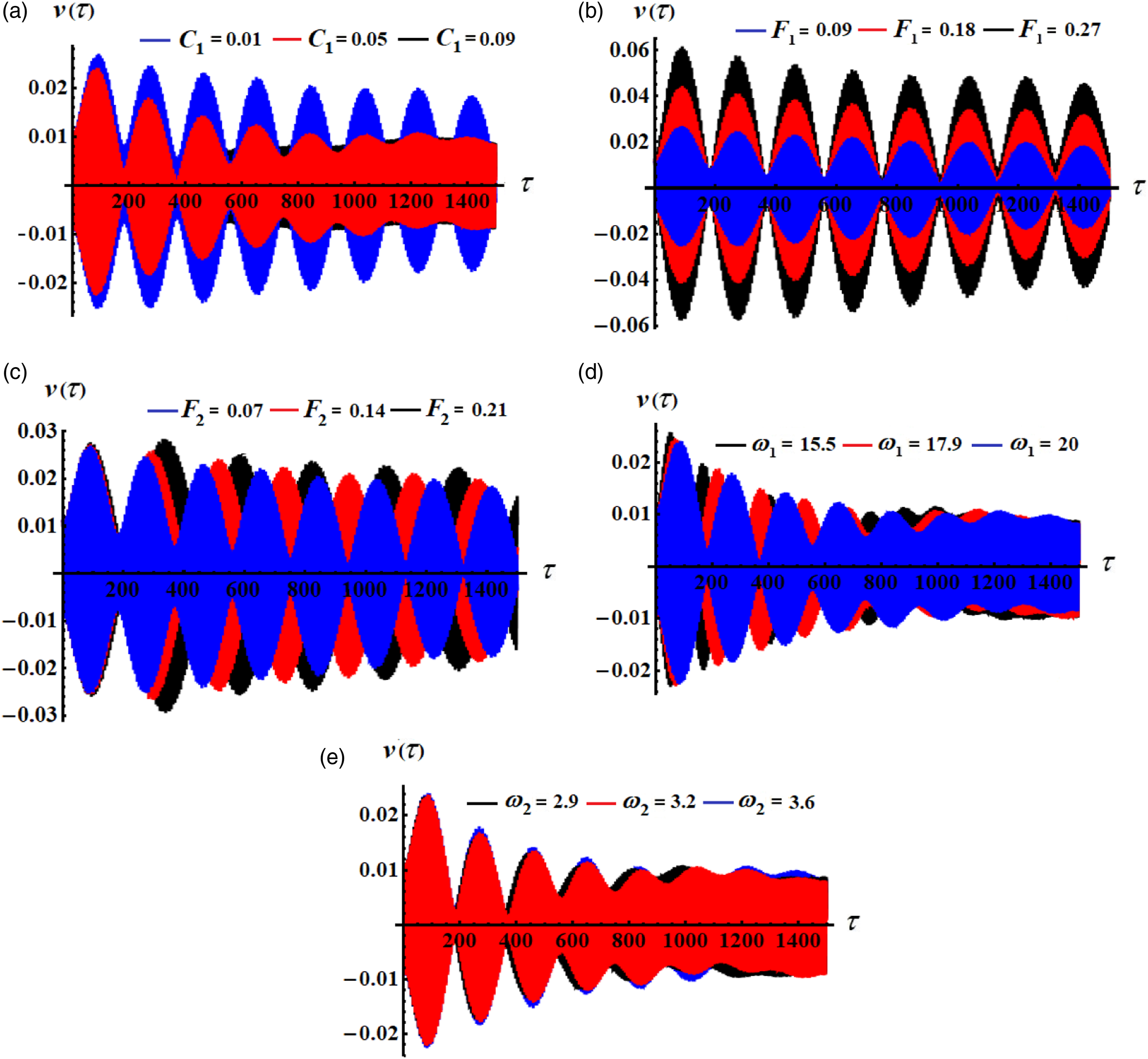
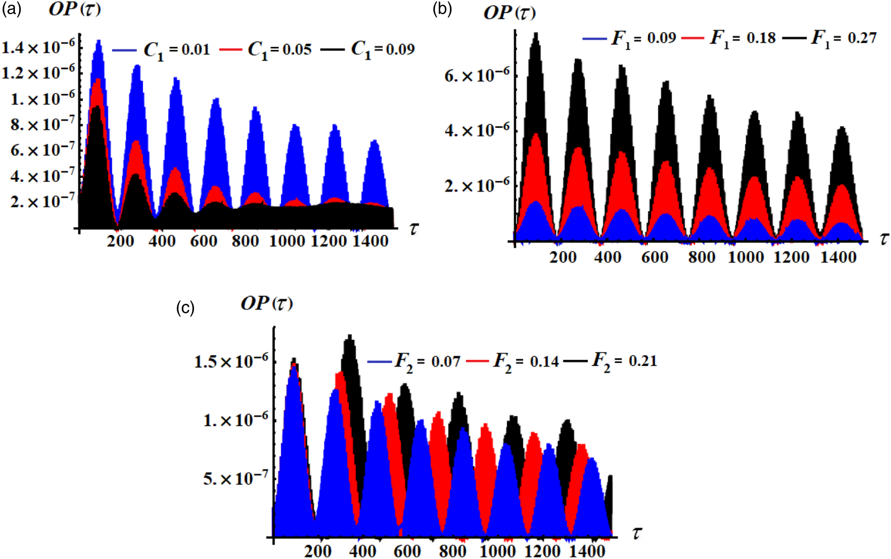
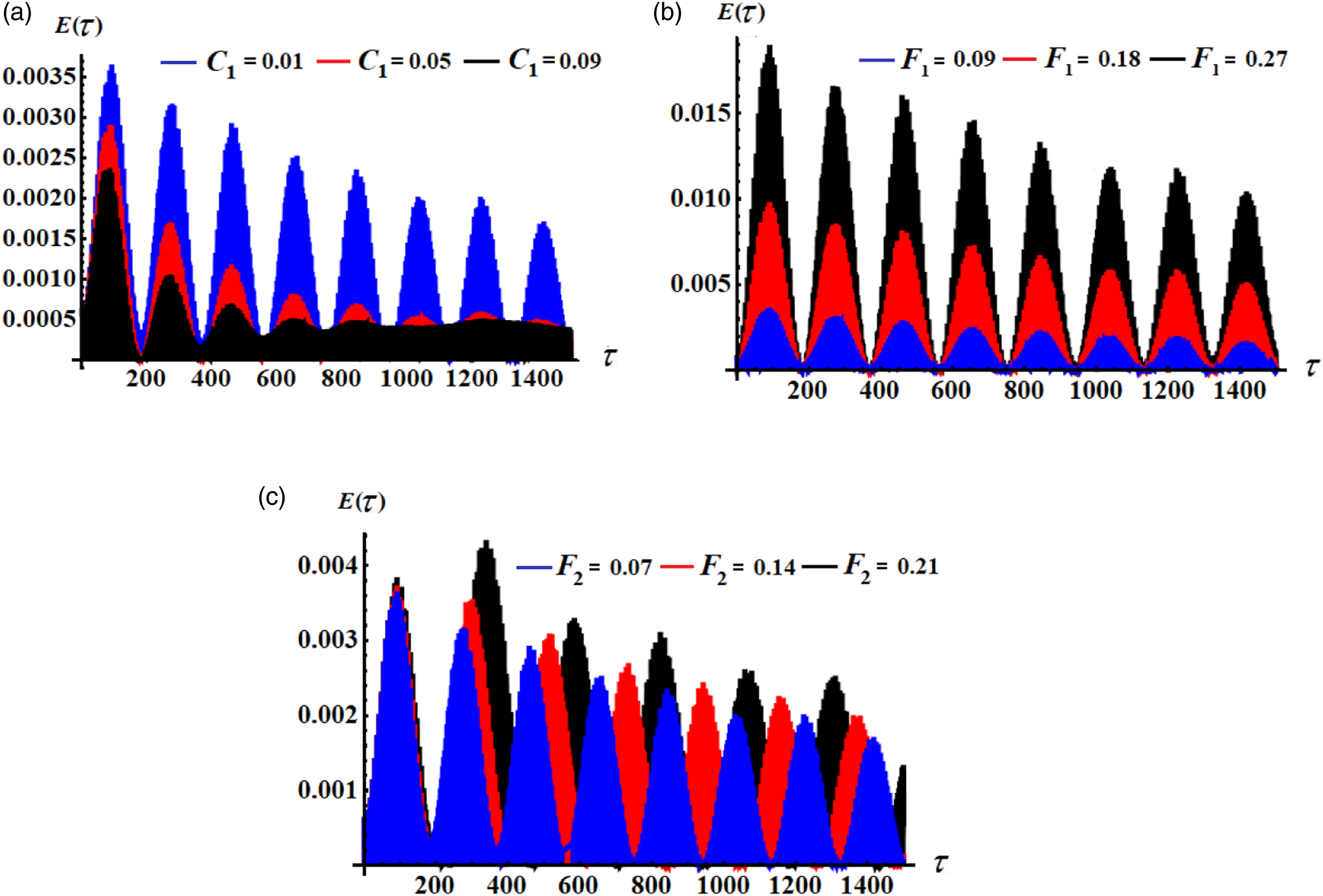
In order to get high performance, we’re going to look at how different values of the used parameters effect on the system. Figures 25–27 illustrate the time histories of the piezoelectric’s output voltages, powers, and energy, respectively. An inspection of the parts of Figure 25 reveals that we have periodic decay of standing waves throughout the whole-time interval. The amplitudes of these waves decrease with the increase of the damping parameter and increase with the values of , respectively, as explored in Figure 25(a) and (b). The impact of various values of and produces periodic decaying waves during the examined interval, as noted in Figure 25(c)–(e). The positive influence of the parameters and on the behavior of the produced power as a result of the piezoelectric device, is drawn in Figure 26. Analyzing the plotted curves in Figure 26 demonstrated that the output power increases and decreases with the increase of the values of and , respectively. The same analyses can be applied on the produced curves in Figure 27 for the output energy , in which this energy decreases with the increase of and increases with the raise values of and .
The voltage’s behavior via at the different values of and .
The temporal behavior of the output power at different values of and .
The energy’s time histories at different values of and .
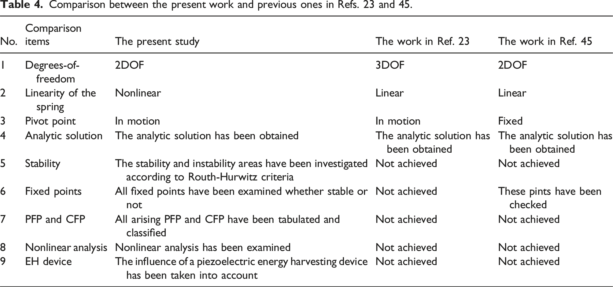
Comparisons with benchmark work with other previous works, for example, Ref. 23 and Ref. 45 is provided in Table 4 to include the design, the state of the pivot point, the number of DOF, the obtained solutions, stability regions, fixed points, CFP, PFP, nonlinear analysis, as well as the EH device.
Comparison between the present work and previous ones in Refs. 23 and 45.
The stability and instability areas have been investigated according to Routh-Hurwitz criteria
Not achieved
Not achieved
6
Fixed points
All fixed points have been examined whether stable or not
Not achieved
These pints have been checked
7
PFP and CFP
All arising PFP and CFP have been tabulated and classified
Not achieved
Not achieved
8
Nonlinear analysis
Nonlinear analysis has been examined
Not achieved
Not achieved
9
EH device
The influence of a piezoelectric energy harvesting device has been taken into account
Not achieved
Not achieved
Conclusions
A novel dynamical system with a 2DOF nonlinear damped oscillating SP system that is coupled to a piezoelectric EH device has been examined, in which its suspension point moves in a Lissajous route with a constant angular velocity. The following results have been listed:
1. The controlling motion’s system has been derived utilizing Lagrange’s equations and solved analytically applying using the MST up to higher approximation to obtain novel analytic solution.
2. The achieved analytic solution has been verified through comparison with the numerical one of the original system of motion, to reveal the great accuracy of the analytic solution and to demonstrate the validity of the MST.
3. The solvability conditions are established once the produced secular words have been removed. Consequently, every resonance case has been categorized. The modulation equations for two of these resonances have been explored concurrently in view of the system’s adjusted phases.
4. From a visual standpoint numerous diagrams showing the temporal histories of the achieved solutions have been analyzed. The gained solutions for the steady-state case have been used to guide the investigation of the nonlinear stability of the modulation equations.
5. The effects of multiple parameters, including damping coefficients, various frequencies, and excitation amplitudes, on the behavior of the system of modulation equations have been thoroughly investigated and analyzed on the outputs of the EH device.
6. To show how the acted-upon parameters influence the system’s behavior, many zones of stability and instability for the FRC have been depicted.
7. The stability and instability zones are and at and , as illustrated in Figure 12.
8. The effect of on seems to be slightly due to the system of equation (42), as indicated in Figure 15(b) and (c).
9. The amplitudes are inversely correlated with the damping coefficients.
10. The piezoelectric device generates volt, Watt, and Watt. hour at and , as graphed in Figures 25–27.
11. Furthermore, the stability of the nonlinear amplitudes of the modulation equations and the characteristics of the nonlinear analysis have been demonstrated in light of the use of complex transformations of the system’s amplitudes.
The piezoelectric device, which is connected to the vibrating system, produces electrical energy, as mentioned above, which is used in some practical applications, like as a source of electricity for sensors, for charging electronic devices, and for other medicinal uses.
Footnotes
Authors’ Contributions
T. S. Amer: Conceptualization, Resources, Methodology, Supervision, Formal analysis, Validation, Reviewing and Editing. Taher A. Bahnasy: Investigation, Methodology, Data duration, Supervision, Corroboration, Validation, Examination, Visualization and Reviewing. H. F. Abosheiaha: Formal analysis, Supervision, Data duration, Examination. A. S. Elameer: Investigation, Formal analysis, Writing-Original draft preparation, Methodology, Visualization and Reviewing. A. Almahalawy: Conceptualization, Supervision, Validation, Examination, Visualization and Reviewing.
Declaration of conflicting interests
The author(s) declared no potential conflicts of interest with respect to the research, authorship, and/or publication of this article.
Funding
The author(s) received no financial support for the research, authorship, and/or publication of this article.
ORCID iD
Taher A Bahnasy
Data availability statement
As no datasets were created or examined for this study, data sharing is not applicable to this work.
Appendix I
Appendix II
References
1.
SodanoHAInmanDJParkG. A Review of power harvesting from vibration using piezoelectric materials. Shock Vib Digest2004; 36(3): 197–205.
2.
BeebySTudorJWhiteN. Energy harvesting vibration sources for microsystems applications. Meas Sci Technol2006; 17(12): R175–R195.
3.
SudevalayamSKulkarniP. Energy harvesting sensor nodes: survey and implications. IEEE Commun Surv Tutorials2011; 13(3): 443–461.
4.
PriyaSInmanDJ. Energy harvesting technologies. Berlin: Springer Science+Business Media, LLC, 2009.
5.
BeebySCaoZAlmussallamA. Kinetic, thermoelectric and solar energy harvesting technologies for smart textiles. Netherlands: Elsevier eBooks, 2013, pp. 306–328.
6.
PozoBGarateJIAraujoJÁ, et al.Energy harvesting technologies and equivalent electronic structural models - review. Electronics2019; 8(5): 486.
7.
KimHSKimJ-HKimJ. A review of piezoelectric energy harvesting based on vibration. Int J Precis Eng Manuf2011; 12(6): 1129–1141.
8.
KecikKMituraALenciS, et al.Energy harvesting from a magnetic levitation system. Int J Non Lin Mech2017; 94: 200–206.
9.
BekMAAmerTSSirwahMA, et al.The vibrational motion of a spring pendulum in a fluid flow. Results Phys2020; 19: 103465.
10.
AmerWSAmerTSHassanSS. Modeling and stability analysis for the vibrating motion of three degrees-of-freedom dynamical system near resonance. Appl Sci2021; 11(24): 11943.
11.
AmerTSBekMAHassanSS, et al.The stability analysis for the motion of a nonlinear damped vibrating dynamical system with three-degrees-of-freedom. Results Phys2021; 28: 104561.
12.
AbadyIMAmerTSGadHM, et al.The asymptotic analysis and stability of 3DOF non-linear damped rigid body pendulum near resonance. Ain Shams Eng J2022; 13(2): 101554.
13.
AmerTSBekMAHassanSS. The dynamical analysis for the motion of a harmonically two degrees of freedom damped spring pendulum in an elliptic trajectory. Alex Eng J2022; 61(2): 1715–1733.
14.
ZhangYYangTDuH, et al.Wideband vibration isolation and energy harvesting based on a coupled piezoelectric-electromagnetic structure. Mech Syst Signal Process2023; 184: 109689.
15.
RoundySWrightPKRabaeyJM. A study of low level vibrations as a power source for wireless sensor nodes. Comput Commun2003; 26(11): 1131–1144.
16.
DutoitNEWardleBLKimSG. Design considerations for MEMS-scale piezoelectric mechanical vibration energy harvesters. Integrated Ferroelectrics Int J2005; 71(1): 121–160.
17.
ChenYYanZ. Nonlinear analysis of axially loaded piezoelectric energy harvesters with flexoelectricity. Int J Mech Sci2020; 173: 105473.
18.
HeC-HAmerTSTianD, et al.Controlling the kinematics of a spring-pendulum system using an energy harvesting device. J Low Freq Noise Vib Act Control2022; 41(3): 1234–1257.
19.
CaoJZhouSInmanDJ, et al.Chaos in the fractionally damped broadband piezoelectric energy generator. Nonlinear Dynam2014; 80(4): 1705–1719.
20.
AbohamerMKAwrejcewiczJStarostaR, et al.Influence of the motion of a spring pendulum on energy-harvesting devices. Appl Sci2021; 11(18): 8658.
21.
BekMAAmerTSAlmahalawyA, et al.The asymptotic analysis for the motion of 3DOF dynamical system close to resonances. Alex Eng J2021; 60(4): 3539–3551.
22.
AmerTSBekMAAbouhmrMK. On the vibrational analysis for the motion of a harmonically damped rigid body pendulum. Nonlinear Dynam2018; 91(4): 2485–2502.
23.
El-SabaaFMAmerTSGadHM, et al.On the motion of a damped rigid body near resonances under the influence of harmonically external force and moments. Results Phys2020; 19: 103352.
24.
AmerTSStarostaRElameerAS, et al.Analyzing the stability for the motion of an unstretched double pendulum near resonance. Appl Sci2021; 11(20): 9520.
25.
AbdelhfeezSAAmerTSElbazRF, et al.Studying the influence of external torques on the dynamical motion and the stability of a 3DOF dynamic system. Alex Eng J2022; 61(9): 6695–6724.
26.
AmerTSEl-SabaaFMZakriaSK, et al.The stability of 3-DOF triple-rigid-body pendulum system near resonances. Nonlinear Dynam2022; 110(2): 1339–1371.
27.
AmerTSStarostaRAlmahalawyA, et al.The stability analysis of a vibrating auto-parametric dynamical system near resonance. Appl Sci2022; 12(3): 1737.
28.
HeJ-HAmerTSAbolilaAF, et al.Stability of three degrees-of-freedom auto-parametric system. Alex Eng J2022; 61(11): 8393–8415.
29.
AmerWSAmerTSStarostaR, et al.Resonance in the cart-pendulum system-an asymptotic approach. Appl Sci2021; 11(23): 11567.
30.
AmerTSBekMANaelMS, et al.Stability of the dynamical motion of a damped 3DOF auto-parametric pendulum system. J Vib Eng Technol2022; 10(5): 1883–1903.
31.
AbohamerMKAwrejcewiczJAmerTS. Modeling of the vibration and stability of a dynamical system coupled with an energy harvesting device. Alex Eng J2023; 63: 377–397.
32.
AbohamerMKAwrejcewiczJAmerTS. Modeling and analysis of a piezoelectric transducer embedded in a nonlinear damped dynamical system. Nonlinear Dynam2023; 111: 8217–8234.
33.
JoyAJoshiVNarendranK, et al.Piezoelectric energy extraction from a cylinder undergoing vortex-induced vibration using internal resonance. Sci Rep2023; 13: 6924.
34.
AlluhydanKNajarFAbdelkefiA. Insights on the performance and dynamical characteristics of piezoelectric energy harvesters with dissipative viscoelastic impacts. Nonlinear Dynam2024; 112: 13027–13046.
35.
TianWHuangJ. Dynamical interaction between double pendulum and nonlinear sloshing in two cranes carrying a liquid tank. Nonlinear Dynam2024; 112: 12705–12720.
36.
Al-SolihatMK. Nonlinear static and dynamic behaviors of partially and fully submerged rod pendulums in quiescent water. Nonlinear Dynam2024; 112: 12907–12924.
37.
AlluhydanKMoatimidGMAmerTS, et al.Inspection of a time-delayed excited damping Duffing oscillator. Axioms2024; 13: 416.
38.
SaeedNAAwrejcewiczJElashmaweyRA, et al.On $$\frac{1}{2}$$-DOF active dampers to suppress multistability vibration of a $$2$$-DOF rotor model subjected to simultaneous multiparametric and external harmonic excitations. Nonlinear Dynam2024; 112: 12061–12094.
39.
AmerTSGalalAA. Vibrational dynamics of a subjected system to external torque and excitation force. J Vib Control2024; 2024: 1–14, DOI: 10.1177/10775463241249618.
40.
AmerTSEl-SabaaFMMoatimidGM, et al.On the stability of a 3DOF vibrating system close to resonances. J Vib Eng Technol2024; 12: 6297–6319.
41.
RajasekarSSanjuánMAF. Nonlinear resonances. Berlin: Springer International Publishing Switzerland, 2016.
42.
StrogatzSH. Nonlinear dynamics and chaos: with applications to physics, biology, chemistry. In: And engineering. 2nd ed.Princeton, NJ, USA: Princeton University Press, 2015.
AmerTSIsmailAIShakerMO, et al.Stability and analysis of the vibrating motion of a four degrees-of-freedom dynamical system near resonance. Control2024; 43(2): 765–795.
45.
StarostaRSypniewska-KamińskaGAwrejcewiczJ. Asymptotic analysis of kinematically excited dynamical systems near resonances. Nonlinear Dynam2012; 68: 459–469.