Sage Journals: Discover world-class research

Abstract

This work focuses on vibration alleviation and energy harvesting in a dynamical system of a spring-pendulum. The structure of the pendulum is modified using an independent electromagnetic harvesting system. The harvesting depends on the oscillation of a magnet in a coil. An endeavor has been made to get both the energy harvesting and mitigation of vibration efficacy of the harvester. The governing kinematics equations are derived using Lagrange’s equations and are solved asymptotically using the multiple scales method to achieve the intended outcome as new and precise results. The resonance states are classified, and the influence of various parameters of the studied system is analyzed. Fixed points at steady states are categorized into stable and unstable. The time behavior of the solutions, the modified amplitudes, and phases are examined and interpreted in the light of their graphical plots. Zones of stability and instability are concerned, in which the system’s behavior is stable for a wide range of used parameters. This model has become essential in recent times as it uses control sensors in industrial applications, buildings, infrastructure, automobiles, and transportation.

Keywords

Harvesting of energy multiple scales method resonance fixed points zones of stability low frequency variational principle

Introduction

In the past few decades, extensive studies have centered on the concept capable of damping harmful vibrations in various sorts of structural engineering: high-rise buildings, bridges, towers, rotary turbines, cables, helicopter feathers, and the robot’s arms.¹ The extensive vibrations are generated by earthquakes, rapid speeds of vehicles, and tremendous winds that may be perilous if they affect the stability and integrity of the structure. Therefore, civil structures require special requirements for vibration alleviation or the addition of isolators between the machine and the excitation generator, modification of the structure to hold vibration far away from resonance positions, or absorption or dispersion of vibration energy using extrinsic apparatus. The primary way to achieve these critical requirements is by dealing with stiffness besides damping control or activating a dynamic vibration absorber (DVA). It can be used to suppress undesired machine vibrations. The simplest form of the DVA consists of a spring-mass-damper (SMD).^2,3

On the other side, vibration energy, which has recently gained much focus, is a sustainable renewable energy source. Vibrations with large amplitudes can be employed to gather energy harvesting (EH), which is also renowned by energy scavenging (ES). It is defined as turning vibrational kinetic energy into serviceable electric energy. Vibration, mechanical strain, and stress are considered sources of energy that can be recovered from mechanical systems. Small devices, including wireless sensors and micro-electromechanical systems (MEMS), can be powered by EH.^4,5

For decades, batteries have been used as the primary power source for mobile electronic gadgets. However, in MEMS, the scaling rate was far faster than in battery technologies.⁶

The lack of built-in and effective power sources has become one of the limitations that enable the increasing use of portable and wireless systems in everyday life; since it is impractical to use large batteries and replace them on a regular basis in specific applications, therefore, the use of EH as a major energy source in tiny systems is the best possible idea. Consequently, temporary energy tanks may be exchanged with continuously charged energy store elements using available energy resources, including sunshine, vibration, and heat.^7–9 Among them, vibration is particularly charming due to its wide uses. Some of the sources of vibrations in environments are vehicle movement and human movements.

Energy can be harvested from these sources using electromagnetic transduction, electrostatic, or piezoelectric. The majority of these vibrations, on the other hand, happen at low frequencies resulting in low power levels at the output; the amount of energy retrieved from these systems is mainly in the order of micro- to milli-watts.^10–13 The low-frequency property also plays a vital role in mass and energy delivery on a nano-/microscale.^14–16

Electromagnetic energy harvesters are instituted on the induction law of Faraday, which states that any change in the magnetic environment of a coil of wire will cause induced electromotive force (EMF) in the coil. It happens according to the magnet’s movement in relation to the coil.¹⁷ Electrostatic transmutation utilizes capacitors to transmit mechanical energy to an electric field. This capacitor can be used as a current source to power an electric circuit.¹⁸ A piezoelectric material will produce an electric field during the piezoelectric processing, and therefore, when deformed under stress, a voltage is produced.¹⁹

The movement of the pivot point of the springe’s pendulum on various trajectories is investigated in several works.^20–24 The motion of a solid body pendulum is analyzed in Refs. 20–22 when the pivot point moves in elliptic paths or in Lissajous curves for different linear or non-linear stiffness cases of the spring. The rigid triple-pendulum motion is checked in Ref. 23 under the action of excitation force and the moment when its attached point moves in a circular path. The estimated results are gained applying the multiple scales method (MSM) up to different orders of approximations. In Ref. 24, the MSM is used to carry out the electromagnetic spring-pendulum harvester model; a two-to-one internal of vibratory energy harvesters are studied.

In Ref. 25, the authors demonstrated the numerical study of an auto-parametric pendulum absorber with a composite harvesting system. Moreover, effective electricity is discussed in relation to the system and various electrical standards. A system of energy harvesting is investigated based on the dynamic pendulum absorber and an electromagnetic harvester in Ref. 26. A new system for simultaneous energy harvesting and vibration dampening is presented in Ref. 27. The absorber was an auto-parametric pendulum, and the energy harvester was a pendulum-mounted electromagnetic harvester. The overall behavior of this new absorber combine harvester was investigated, and the results indicated that the harvester did not decrease the vibration reduction efficiency. It has been observed that energy can be harvested for the rotation of the pendulum and chaotic motion. A pendulum system with two independent electromagnetic harvesters has been introduced in Ref. 28. A direct current (DC) electric motor is added to the pendulum’s axis to be a second harvesting machine. The results revealed that the suggested system is greatly increasing the capacity of EH. However, the rotary harvester has lessened the vibration suppression efficiency. In Ref. 29, the vibration absorber was developed into an energy harvesting device and vibration absorbing system to suppress undesired vibrations and to produce an induced voltage that could be used in low voltage applications such as wireless sensors. In Ref. 30, numerical analysis of a semi-active suspension mounted absorber or harvested system has been studied, in which the primary objective is used to damp the primary structure’s vibration and the secondary objective is to simultaneously harvest energy from the absorber’s vibration. The pendulum-tuned mass absorber is adjusted by a magnetic levitation harvester. In Ref. 31, the authors studied the effect of EH and control of vibrations by a specially designed pendulum absorber in addition to the use of non-linear vibration absorbers as an energy harvester. The use of an energy recovery device has been shown to increase vibration reduction in the low-frequency range. In Ref. 32, the authors focus on a new pendulum absorber harvester configuration that permits for amended shaking suppression and EH properties. The new absorber structure refers to the use of magnets, its performance is studied theoretically and empirically, and the outcomes demonstrate that the new absorber harvester has a better performance than the traditional device regarding both vibration suppression and EH. The authors investigated in Ref. 33 the motion of an axial pendulum model, which is based on a coupled 2DOF dynamical model that respects two horizontal and vertical axes of the pendulum.

The method of harmonic balance (MHB) is applied in Refs. 34, 35 to illustrate the response and stability of EH electrical and mechanical systems, in which the harvesting system is made up of two similar magnets placed securely at the tube’s end. Between them, a third magnet is magnetically free to ascend. The influence of the parameters of the harvester on system responsiveness and energy recovery around the most important resonance has been thoroughly investigated.

In this paper, we present a simple apparatus based on spring oscillations for harvesting energy from oscillating environments. A power generator converts the mechanical energy of a spring into an electric one, which can be utilized in a variety of applications, including automotive,³⁶ wireless sensor networks (WSNs),³⁷ health-monitoring devices,³⁸ and structural engineering.³⁹ The researched system’s mathematical model and operating principles are provided. The MSM is being utilized to gain the desired solutions that are matching to the system’s generalized coordinates. The modulation equations are acquired in light of the emerging cases of resonance. The dynamic response curves of the resonance are examined through some plots at values close to the resonance regions, in which the stability of the considered system is examined. The historical variations of the achieved solutions with time are performed. The adjusted phases and the amplitudes are presented to demonstrate the efficacy of the physical parameters at any given moment, where the plots of their phase planes are presented to confirm that we have stable fixed points in these cases of steady state. The types of these points were checked in terms of their stabilities. The non-linear stability analysis of Routh–Hurwitz is examined and discussed.

The problem’s description

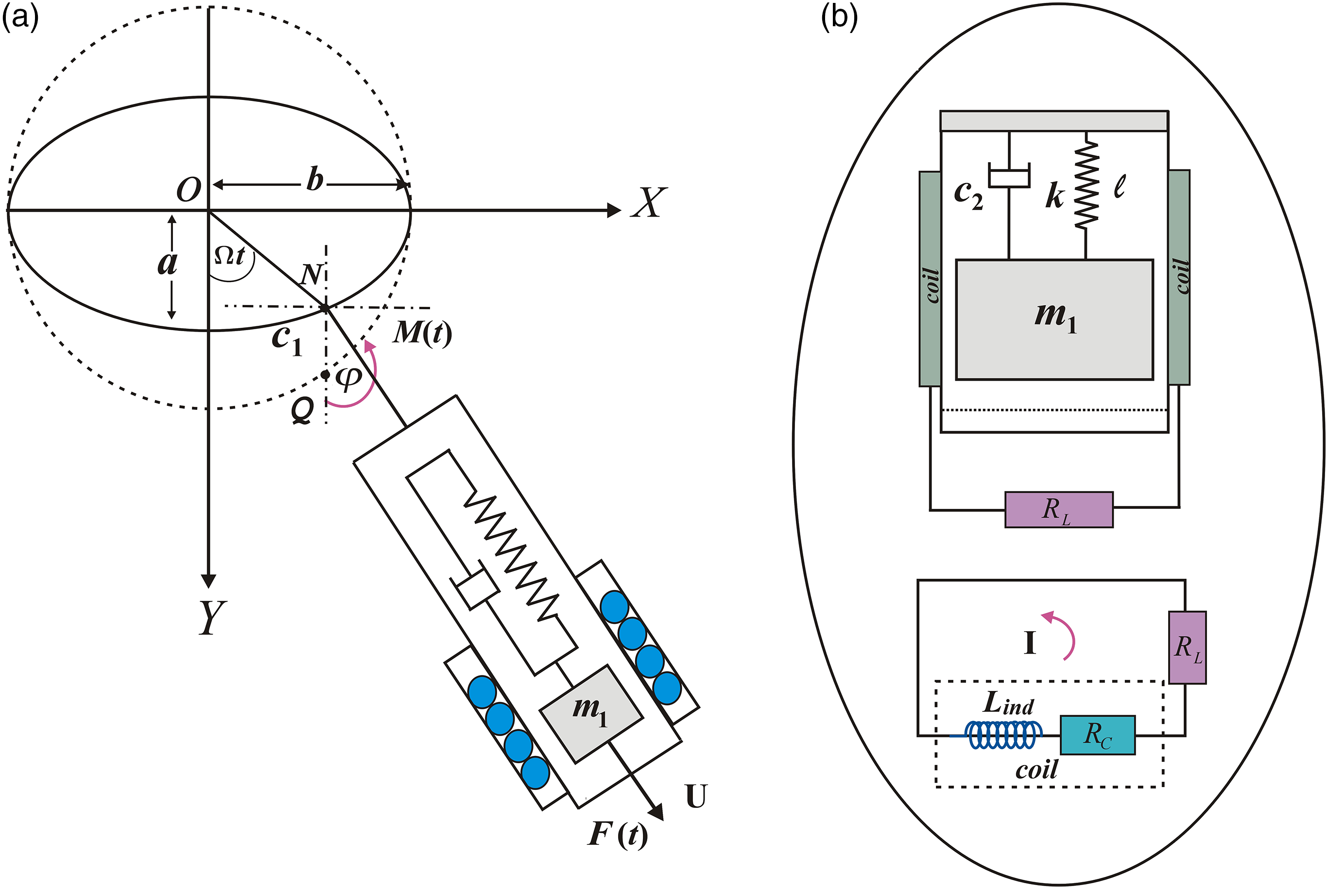
This section is proceeded to describe the investigated model. Therefore, let us consider an advanced harvester comprised of a cylindrical tube with two imperishable magnets attached inside the tube at its ends, besides a third movable magnet with a mass $m_{1}$ that is attached to a massless linear spring with stiffness $k$ , damping coefficient $c_{2}$ , and non-extended length $ℓ$ . A harmonic excitation force $F (t)$ is imposed upon the magnet beside a moment $M (t)$ acting on the suspension point $N$ of the spring. This point is only allowed to move in an elliptic trajectory with minor and major axes $2 a$ and $2 b$ , respectively. Let a point $Q$ be a projection of the point $N$ on a supplementary circle $b$ in which it moves with a constant angular velocity $Ω$ (see Figure 1(a)). Therefore, the kinematics coordinates of the point $N$ can be written as follows

X_{N} = b \sin (Ω t), Y_{N} = a \cos (Ω t) .

(1)

Figure 1.

(a) A schematic diagram of spring-pendulum with an energy harvester and (b) the harvester model with an electric circuit.

Let $c_{1}$ represents the rotatory damping coefficient of the spring at the rotatory point, $I$ denotes the current due to the oscillations of the magnet in a coil, the harvester electric component composed of $R_{L}$ which points to the load resistance of the resistor, $L_{ind}$ refers to the coil’s inductance, $R_{C}$ is the coil’s resistance, and $L_{coil}$ express the coil length (see Figure 1(b)).

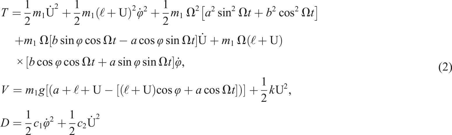
To derive the equations of motion (EOM), we consider that the variables $U$ and $φ$ describe the extension of the spring and the rotatory angle, respectively. Therefore, the kinetic energy $T$ , the potential one $V$ , and the dissipation function $D$ can be expressed as

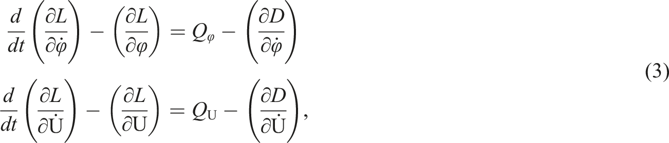
\begin{array}{l} T = \frac{1}{2} m_{1} {\dot{U}}^{2} + \frac{1}{2} m_{1} {(ℓ + U)}^{2} {\dot{φ}}^{2} + \frac{1}{2} m_{1} Ω^{2} [a^{2} \sin^{2} Ω t + b^{2} \cos^{2} Ω t] \\ + m_{1} Ω [b \sin φ \cos Ω t - a \cos φ \sin Ω t] \dot{U} + m_{1} Ω (ℓ + U) \\ \times [b \cos φ \cos Ω t + a \sin φ \sin Ω t] \dot{φ}, \\ V = m_{1} g [(a + ℓ + U - [(ℓ + U) \cos φ + a \cos Ω t])] + \frac{1}{2} k U^{2}, \\ D = \frac{1}{2} c_{1} {\dot{φ}}^{2} + \frac{1}{2} c_{2} {\dot{U}}^{2} \end{array}

(2)

Based on (2) and Lagrange’s functions $L = T - V$ , we can derive the EOM according to the below equations of Lagrange^40–42

\begin{matrix} \frac{d}{d t} (\frac{\partial L}{\partial \dot{φ}}) - (\frac{\partial L}{\partial φ}) = Q_{φ} - (\frac{\partial D}{\partial \dot{φ}}) \\ \frac{d}{d t} (\frac{\partial L}{\partial \dot{U}}) - (\frac{\partial L}{\partial U}) = Q_{U} - (\frac{\partial D}{\partial \dot{U}}), \end{matrix}

(3)

where

Q_{U}

and

Q_{φ}

are the generalized forces

\begin{array}{l} Q_{φ} = M (t) = M_{0} (t) \cos (Ω_{1} t), \\ Q_{U} = F (t) = F_{0} \cos (Ω_{2} t) \end{array}

(4)

Here, $M_{0}, F_{0}$ and $Ω_{1}, Ω_{2}$ are the amplitudes and the frequencies of the moment $M (t)$ and the external force $F (t)$ , respectively.

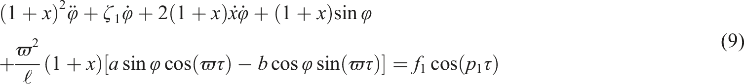
Substituting (2) and (4) into (3) produces the EOM as in the following non-dimensional form

\begin{array}{l} m_{1} {(ℓ + U)}^{2} \ddot{φ} + c_{1} \dot{φ} + 2 m_{1} (ℓ + U) \dot{U} \dot{φ} + m_{1} g (ℓ + U) \sin φ \\ + m_{1} Ω^{2} (ℓ + U) [a \sin φ \cos (Ω t) - b \cos φ \sin (Ω t)] = M_{0} (t) \cos (Ω_{1} t) \end{array}

(5)

\begin{array}{l} m_{1} \ddot{U} + c_{2} \dot{U} + k U + m_{1} g (1 - \cos φ) - m_{1} (ℓ + U) {\dot{φ}}^{2} \\ - m_{1} Ω^{2} [b \sin φ \sin (Ω t) + a \cos φ \cos (Ω t)] + Β L_{coil} Ι = F_{0} \cos (Ω_{2} t) \end{array}

(6)

where dots are the time derivatives.

Applying Kirchhoff Volt Law (KVL) and Faraday’s one²⁴ of the electromagnetic induction for the circuit of Figure 1(b), then we can write

L_{ind} \dot{Ι} + R Ι - Β L_{coil} \dot{U} = 0

(7)

where

R

is the summation of the load resistance

R_{L}

and the coil’s resistance

R_{C}

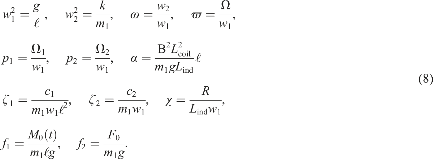
Inserting a dimensionless time parameter $τ = w_{1} t$ , dimensionless coordinates $x = U / ℓ,$ $Z = (L_{ind} / B L_{coil} ℓ) Ι,$ $φ = φ$ besides the following dimensionless parameters

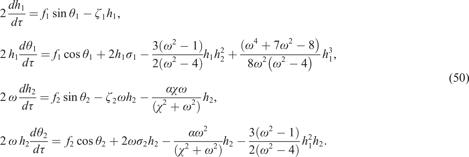
\begin{array}{l} w_{1}^{2} = \frac{g}{ℓ}, w_{2}^{2} = \frac{k}{m_{1}}, ω = \frac{w_{2}}{w_{1}}, ϖ = \frac{Ω}{w_{1}}, \\ p_{1} = \frac{Ω_{1}}{w_{1}}, p_{2} = \frac{Ω_{2}}{w_{1}}, α = \frac{Β^{2} L_{coil}^{2}}{m_{1} g L_{ind}} ℓ \\ ζ_{1} = \frac{c_{1}}{m_{1} w_{1} ℓ^{2}}, ζ_{2} = \frac{c_{2}}{m_{1} w_{1}}, χ = \frac{R}{L_{ind} w_{1}}, \\ f_{1} = \frac{M_{0} (t)}{m_{1} ℓ g}, f_{2} = \frac{F_{0}}{m_{1} g} . \end{array}

(8)

Substitution of (8) into (5), (6), and (7) yields the following dimensionless forms of the EOM

\begin{array}{l} {(1 + x)}^{2} \ddot{φ} + ζ_{1} \dot{φ} + 2 (1 + x) \dot{x} \dot{φ} + (1 + x) \sin φ \\ + \frac{ϖ^{2}}{ℓ} (1 + x) [a \sin φ \cos (ϖ τ) - b \cos φ \sin (ϖ τ)] = f_{1} \cos (p_{1} τ) \end{array}

(9)

\begin{array}{l} \ddot{x} + ζ_{2} \dot{x} + ω^{2} x + (1 - \cos φ) - (1 + x) {\dot{φ}}^{2} \\ - \frac{ϖ^{2}}{ℓ} [b \sin φ \sin (ϖ τ) + a \cos φ \cos (ϖ τ)] + α Z = f_{2} \cos (p_{2} τ) \end{array}

(10)

\dot{Z} + χ Z - \dot{x} = 0

(11)

where dots denote the differentiation with respect to

τ

. The above three equations are considered as non-linear second-order differential equations.

Asymptotic method of the solutions

The main objective of this part is to get the desired solutions to the EOM of the preceding system (9)–(11) up to higher order of approximation using one of the significant perturbation approaches known by the multiple scales method (MSM) and to classify the resonance cases.²² It should be pointed out that non-Gaussian random vibration test can also be applied effectively.^43–45

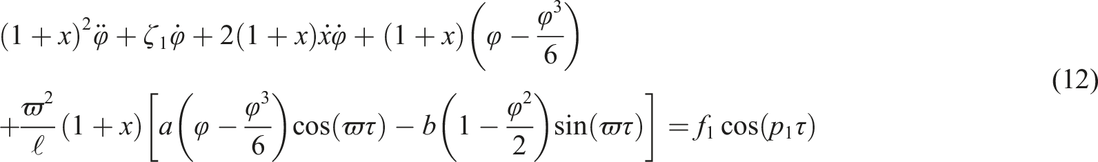
To realize this objective, we approximate the functions $\sin φ$ and $\cos φ$ up to third-order using the Taylor series, which are valid in close proximity to static equilibrium. Therefore, equations (9)–(11) can be rewritten in the form

\begin{array}{l} {(1 + x)}^{2} \ddot{φ} + ζ_{1} \dot{φ} + 2 (1 + x) \dot{x} \dot{φ} + (1 + x) (φ - \frac{φ^{3}}{6}) \\ + \frac{ϖ^{2}}{ℓ} (1 + x) [a (φ - \frac{φ^{3}}{6}) \cos (ϖ τ) - b (1 - \frac{φ^{2}}{2}) \sin (ϖ τ)] = f_{1} \cos (p_{1} τ) \end{array}

(12)

\ddot{x} + ζ_{2} \dot{x} + ω^{2} x + \frac{φ^{2}}{2} - (1 + x) {\dot{φ}}^{2} - \frac{ϖ^{2}}{ℓ} [b (φ - \frac{φ^{3}}{6}) \sin (ϖ τ) + a (1 - \frac{φ^{2}}{2}) \cos (ϖ τ)] + α Z = f_{2} \cos (p_{2} τ)

(13)

\dot{Z} + χ Z - \dot{x} = 0

(14)

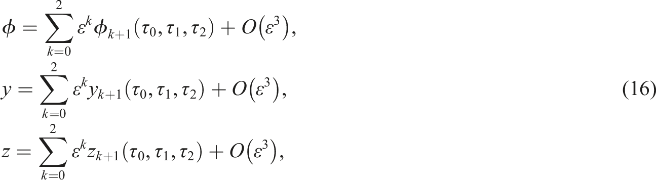
We assume that the generalized coordinates can be expressed in terms of the order $0 < ε < < 1$ . Therefore, we consider new variables $ϕ, y$ , and $z$ as follows

φ (τ) = ε ϕ (τ; ε), x (τ) = ε y (τ; ε), Z (τ) = ε z (τ; ε),

(15)

According to MS procedure, we can introduce the functions $ϕ, y$ , and $z$ in powers of $ε$ as follows

\begin{array}{l} ϕ = \sum_{k = 0}^{2} ε^{k} ϕ_{k + 1} (τ_{0}, τ_{1}, τ_{2}) + O (ε^{3}), \\ y = \sum_{k = 0}^{2} ε^{k} y_{k + 1} (τ_{0}, τ_{1}, τ_{2}) + O (ε^{3}), \\ z = \sum_{k = 0}^{2} ε^{k} z_{k + 1} (τ_{0}, τ_{1}, τ_{2}) + O (ε^{3}), \end{array}

(16)

where

τ_{n} = ε^{n} τ (n = 0,1,2)

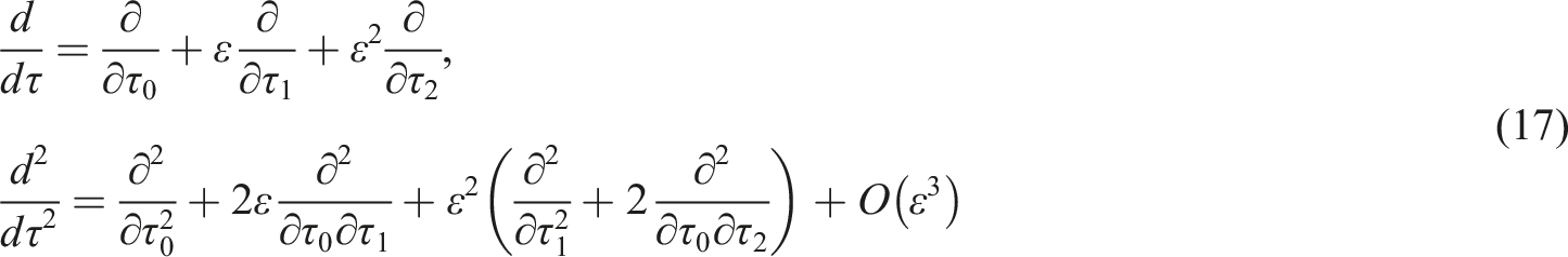
perform diverse time scales, where

τ_{0}

and

τ_{1}, τ_{2}

act as the fast and slow scales, respectively. To define

ϕ, y

, and

z

as functions of

τ_{n}

, we transform

τ

τ_{n}

according to the following operators

\begin{array}{l} \frac{d}{d τ} = \frac{\partial}{\partial τ_{0}} + ε \frac{\partial}{\partial τ_{1}} + ε^{2} \frac{\partial}{\partial τ_{2}}, \\ \frac{d^{2}}{d τ^{2}} = \frac{\partial^{2}}{\partial τ_{0}^{2}} + 2 ε \frac{\partial^{2}}{\partial τ_{0} \partial τ_{1}} + ε^{2} (\frac{\partial^{2}}{\partial τ_{1}^{2}} + 2 \frac{\partial^{2}}{\partial τ_{0} \partial τ_{2}}) + O (ε^{3}) \end{array}

(17)

It is worthwhile to notice that terms of $O (ε^{3})$ and higher are negligent because to their smallness.

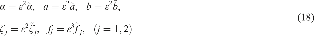
The coefficients of damping and the generalized forces are given in terms of $ε$ as follows

\begin{array}{l} α = ε^{2} \tilde{α}, a = ε^{2} \tilde{a}, b = ε^{2} \tilde{b}, \\ ζ_{j} = ε^{2} {\tilde{ζ}}_{j}, f_{j} = ε^{3} {\tilde{f}}_{j}, (j = 1,2) \end{array}

(18)

where the parameters

\tilde{α}, \tilde{a}, \tilde{b}, {\tilde{ζ}}_{j}

, and

{\tilde{f}}_{j}

are of unity order.

Substituting (15)–(18) into (12)–(14) and equaling the coefficients of distinct powers of $ε, ε^{2}$ , and $ε^{3}$ , to yield the below groups of partial differential equations (PDEs).

Order of $ε$

\frac{\partial^{2} ϕ_{1}}{\partial τ_{0}^{2}} + ϕ_{1} = 0

(19)

\frac{\partial^{2} y_{1}}{\partial τ_{0}^{2}} + ω^{2} y_{1} = 0

(20)

\frac{\partial z_{1}}{\partial τ_{0}} + χ z_{1} = \frac{\partial y_{1}}{\partial τ_{0}}

(21)

Order of $ε^{2}$

\frac{\partial^{2} ϕ_{2}}{\partial τ_{0}^{2}} + φ_{2} = - 2 [\frac{\partial^{2} ϕ_{1}}{\partial τ_{0} \partial τ_{1}} + y_{1} \frac{\partial^{2} ϕ_{1}}{\partial τ_{0}^{2}} + \frac{\partial y_{1}}{\partial τ_{0}} \frac{\partial ϕ_{1}}{\partial τ_{0}}] - y_{1} ϕ_{1} + \frac{ϖ^{2}}{ℓ} \tilde{b} \sin (ϖ τ_{0})

(22)

\frac{\partial^{2} y_{2}}{\partial τ_{0}^{2}} + ω^{2} y_{2} = - 2 \frac{\partial^{2} y_{1}}{\partial τ_{0} τ_{1}} + {(\frac{\partial ϕ_{1}}{\partial τ_{0}})}^{2} - \frac{1}{2} ϕ_{1}^{2} + \frac{ϖ^{2}}{ℓ} \tilde{a} \cos (ϖ τ_{0})

(23)

\frac{\partial z_{2}}{\partial τ_{0}} + χ z_{2} = \frac{\partial y_{2}}{\partial τ_{0}} - \frac{\partial z_{1}}{\partial τ_{1}} + \frac{\partial y_{1}}{\partial τ_{1}}

(24)

Order of $ε^{3}$

\begin{array}{l} \frac{\partial^{2} ϕ_{3}}{\partial τ_{0}^{2}} + ϕ_{3} = {\tilde{f}}_{1} \cos (p_{1} τ_{0}) - \frac{ϖ^{2}}{ℓ} \tilde{a} ϕ_{1} \cos (ϖ τ_{0}) + \frac{ϖ^{2}}{ℓ} \tilde{b} y_{1} \sin (ϖ τ_{0}) \\ - 2 (\frac{\partial^{2} ϕ_{1}}{\partial τ_{0} \partial τ_{2}} + \frac{\partial^{2} ϕ_{2}}{\partial τ_{0} \partial τ_{1}}) - 2 (y_{1} \frac{\partial^{2} ϕ_{2}}{\partial τ_{0}^{2}} + y_{2} \frac{\partial^{2} ϕ_{1}}{\partial τ_{0}^{2}}) - 4 y_{1} \frac{\partial^{2} ϕ_{1}}{\partial τ_{0} \partial τ_{1}} \\ - y_{1}^{2} \frac{\partial^{2} ϕ_{1}}{\partial τ_{0}^{2}} - {\tilde{ζ}}_{1} \frac{\partial ϕ_{1}}{\partial τ_{0}} - 2 y_{1} \frac{\partial y_{1}}{\partial τ_{0}} \frac{\partial ϕ_{1}}{\partial τ_{0}} - 2 (\frac{\partial y_{1}}{\partial τ_{0}} \frac{\partial ϕ_{2}}{\partial τ_{0}} + \frac{\partial y_{1}}{\partial τ_{1}} \frac{\partial ϕ_{1}}{\partial τ_{0}} + \frac{\partial y_{2}}{\partial τ_{0}} \frac{\partial ϕ_{1}}{\partial τ_{0}} + \frac{\partial y_{1}}{\partial τ_{0}} \frac{\partial ϕ_{1}}{\partial τ_{1}}) - y_{1} ϕ_{2} - y_{2} ϕ_{1} + \frac{1}{6} ϕ_{1}^{3} - \frac{\partial^{2} ϕ_{1}}{\partial τ_{1}^{2}}, \end{array}

(25)

\begin{array}{l} \frac{\partial^{2} y_{3}}{\partial τ_{0}^{2}} + ω^{2} y_{3} = {\tilde{f}}_{2} \cos (p_{2} τ_{0}) + \frac{ϖ^{2}}{ℓ} \tilde{b} ϕ_{1} \sin (ϖ τ_{0}) - \frac{\partial^{2} y_{1}}{\partial τ_{1}^{2}} \\ - 2 (\frac{\partial^{2} y_{1}}{\partial τ_{0} \partial τ_{2}} + \frac{\partial^{2} y_{2}}{\partial τ_{0} \partial τ_{1}}) - {\tilde{ζ}}_{2} \frac{\partial y_{1}}{\partial τ_{0}} + y_{1} {(\frac{\partial ϕ_{1}}{\partial τ_{0}})}^{2} \\ - ϕ_{1} ϕ_{2} - \tilde{α} z_{1} + 2 (\frac{\partial ϕ_{1}}{\partial τ_{0}} \frac{\partial ϕ_{2}}{\partial τ_{0}} + \frac{\partial ϕ_{1}}{\partial τ_{0}} \frac{\partial ϕ_{1}}{\partial τ_{1}}) \end{array}

(26)

\begin{array}{l} \frac{\partial z_{3}}{\partial τ_{0}} + χ z_{3} = \frac{\partial y_{3}}{\partial τ_{0}} - (\frac{\partial z_{2}}{\partial τ_{1}} + \frac{\partial z_{1}}{\partial τ_{2}}) + \frac{\partial y_{2}}{\partial τ_{1}} + \frac{\partial y_{1}}{\partial τ_{2}} \end{array}

(27)

It is worthy to remark that the above three systems of orders of $ε$ constitute nine PDEs that can be solved sequentially. To acquire this goal, we begin with the general equations (19)–(21), which can be written as follows

ϕ_{1} = Α_{1} e^{i τ_{0}} + {\bar{Α}}_{1} e^{- i τ_{0}}

(28)

y_{1} = Α_{2} e^{i ω τ_{0}} + {\bar{Α}}_{2} e^{- i ω τ_{0}}

(29)

To get the general solution of $z_{1}$ , substituting (29) into (21) to obtain a nonhomogeneous PDE which can be solved in the form

z_{1} = B_{1} e^{- χ τ_{0}} + \frac{i ω}{χ + i ω} Α_{2} e^{i ω τ_{0}} - \frac{i ω}{χ - i ω} {\bar{Α}}_{2} e^{- i ω τ_{0}}; i = \sqrt{- 1}

(30)

where

Α_{j} (j = 1,2)

and

B_{1}

are complex functions of the slow scales

τ_{1}

and

τ_{2}

, whereas

{\bar{Α}}_{j}

points to their complex conjugates.

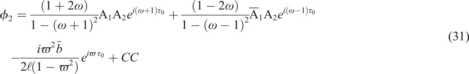
Substituting (28)–(30) into (22)–(24) and removing terms that give secular terms to obtain uniform asymptotic solutions. Then, the second-order solutions have the forms

\begin{array}{l} ϕ_{2} = \frac{(1 + 2 ω)}{1 - {(ω + 1)}^{2}} Α_{1} Α_{2} e^{i (ω + 1) τ_{0}} + \frac{(1 - 2 ω)}{1 - {(ω - 1)}^{2}} {\bar{Α}}_{1} Α_{2} e^{i (ω - 1) τ_{0}} \\ - \frac{i ϖ^{2} \tilde{b}}{2 ℓ (1 - ϖ^{2})} e^{i ϖ τ_{0}} + C C \end{array}

(31)

y_{2} = \frac{- 3 Α_{1}^{2}}{2 (ω^{2} - 4)} e^{2 i τ_{0}} + \frac{ϖ^{2} \tilde{a}}{2 ℓ (ω^{2} - ϖ^{2})} e^{i ϖ τ_{0}} + \frac{1}{ω^{2}} Α_{1} {\bar{Α}}_{1} + C C

(32)

z_{2} = \frac{- 3 i}{(χ + 2 i) (ω^{2} - 4)} Α_{1}^{2} e^{2 i τ_{0}} + \frac{i ϖ^{3} \tilde{a}}{2 ℓ (ω^{2} - ϖ^{2}) (χ + i ϖ)} e^{i ϖ τ_{0}} + C C

(33)

where

C C

indicates the conjugates of the former terms.

Based on the above, we can find the conditions for canceling secular terms from the second approximations in the forms

\frac{\partial Α_{1}}{\partial τ_{1}} = 0, \frac{\partial Α_{2}}{\partial τ_{1}} = 0, \frac{\partial B_{1}}{\partial τ_{1}} = 0

(34)

Therefore, the functions $Α_{j} (j = 1,2)$ and $B_{1}$ depend on $τ_{2}$ only.

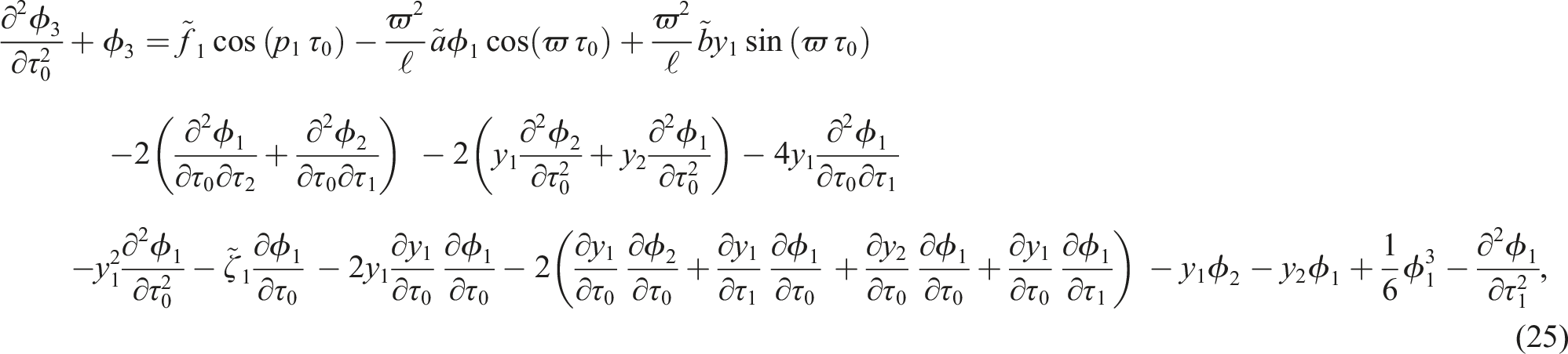
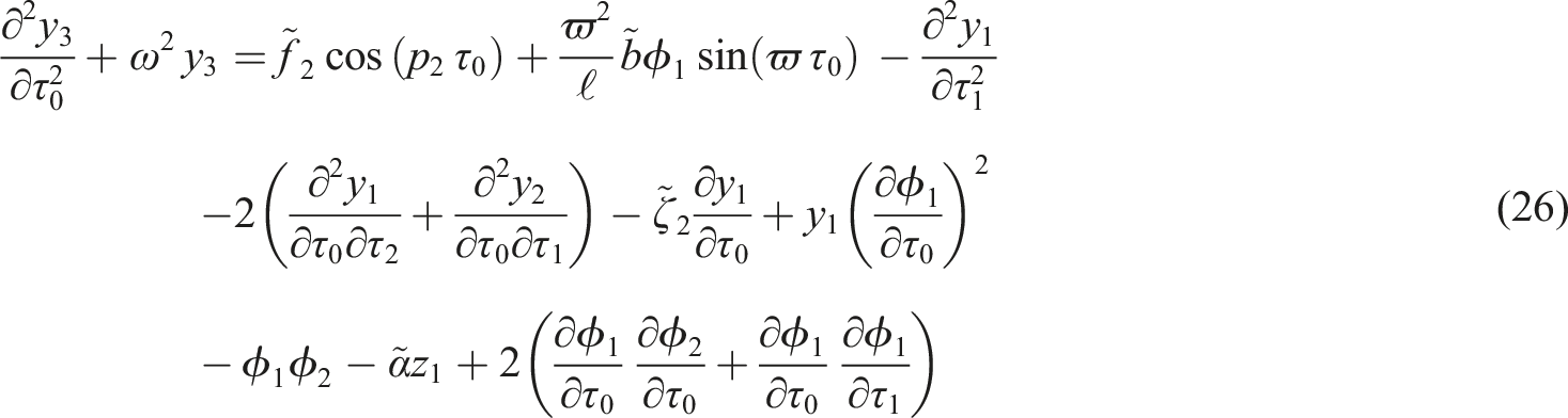
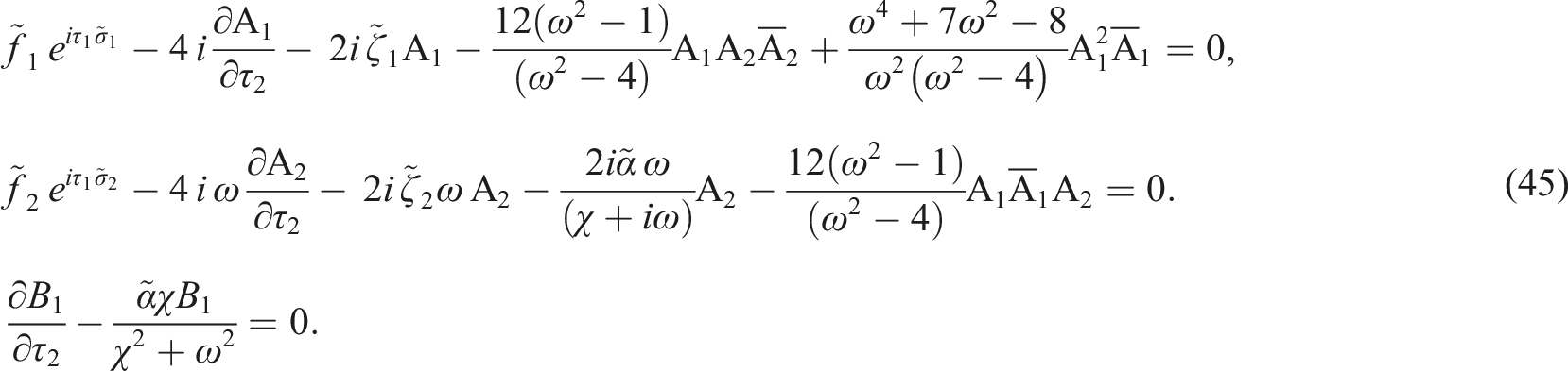
Substituting (28)–(30) and (31)–(34) into (25)–(27) and then canceling terms that yield secular ones to gain the solutions of the third-order approximations. To remove these terms, the following conditions must be satisfied

2 i \frac{\partial Α_{1}}{\partial τ_{2}} + i {\tilde{ζ}}_{1} Α_{1} + \frac{6 (ω^{2} - 1)}{(ω^{2} - 4)} Α_{1} Α_{2} {\bar{Α}}_{2} - \frac{ω^{4} + 7 ω^{2} - 8}{2 ω^{2} (ω^{2} - 4)} Α_{1}^{2} {\bar{Α}}_{1} = 0

(35)

2 i ω \frac{\partial Α_{2}}{\partial τ_{2}} + i {\tilde{ζ}}_{2} ω Α_{2} + \frac{i \tilde{α} ω}{(χ + i ω)} Α_{2} + \frac{6 (ω^{2} - 1)}{(ω^{2} - 4)} Α_{1} {\bar{Α}}_{1} Α_{2} = 0

(36)

\frac{\partial B_{1}}{\partial τ_{2}} - \frac{\tilde{α} χ B_{1}}{χ^{2} + ω^{2}} = 0

(37)

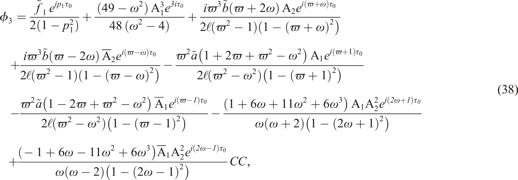
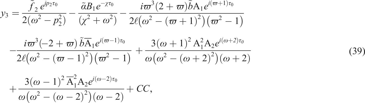
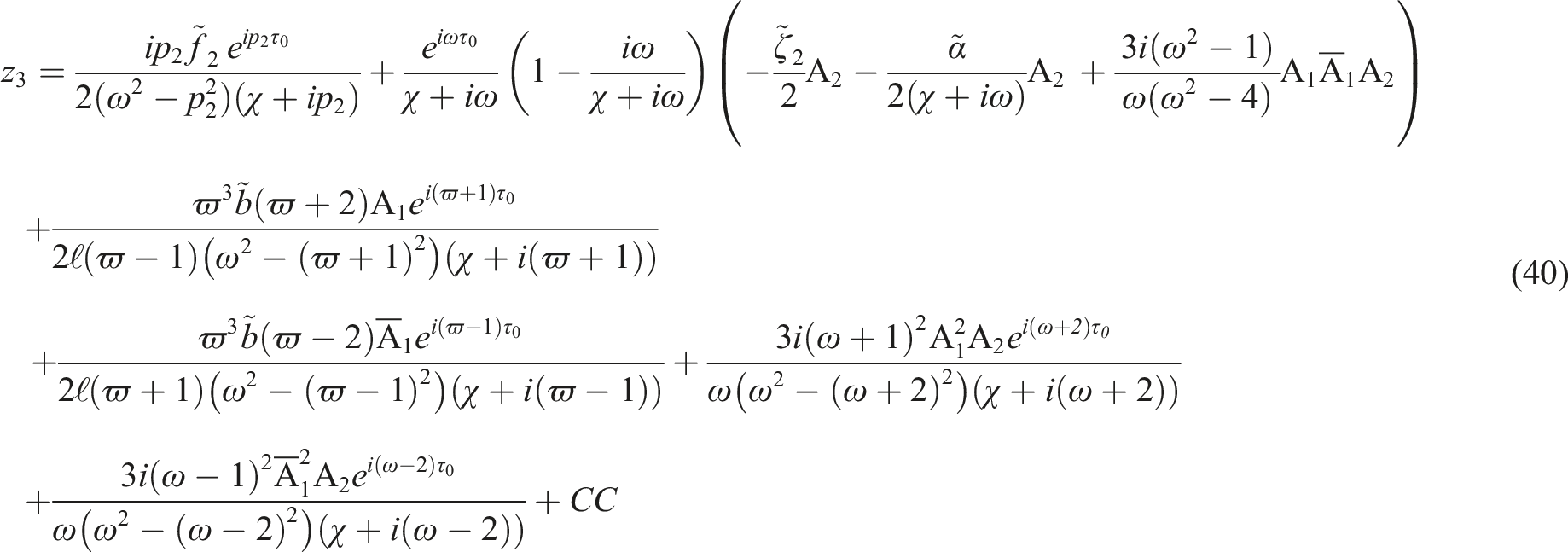
Then, the solutions of the third approximations $ϕ_{3}, y_{3}$ , and $z_{3}$ have the forms

\begin{array}{l} ϕ_{3} = \frac{{\tilde{f}}_{1} e^{i p_{1} τ_{0}}}{2 (1 - p_{1}^{2})} + \frac{(49 - ω^{2}) Α_{1}^{3} e^{3 i τ_{0}}}{48 (ω^{2} - 4)} + \frac{i ϖ^{3} \tilde{b} (ϖ + 2 ω) Α_{2} e^{i (ϖ + ω) τ_{0}}}{2 ℓ (ϖ^{2} - 1) (1 - {(ϖ + ω)}^{2})} \\ + \frac{i ϖ^{3} \tilde{b} (ϖ - 2 ω) {\bar{Α}}_{2} e^{i (ϖ - ω) τ_{0}}}{2 ℓ (ϖ^{2} - 1) (1 - {(ϖ - ω)}^{2})} - \frac{ϖ^{2} \tilde{a} (1 + 2 ϖ + ϖ^{2} - ω^{2}) Α_{1} e^{i (ϖ + 1) τ_{0}}}{2 ℓ (ϖ^{2} - ω^{2}) (1 - {(ϖ + 1)}^{2})} \\ - \frac{ϖ^{2} \tilde{a} (1 - 2 ϖ + ϖ^{2} - ω^{2}) {\bar{Α}}_{1} e^{i (ϖ - 1) τ_{0}}}{2 ℓ (ϖ^{2} - ω^{2}) (1 - {(ϖ - 1)}^{2})} - \frac{(1 + 6 ω + 11 ω^{2} + 6 ω^{3}) Α_{1} Α_{2}^{2} e^{i (2 ω + 1) τ_{0}}}{ω (ω + 2) (1 - {(2 ω + 1)}^{2})} \\ + \frac{(- 1 + 6 ω - 11 ω^{2} + 6 ω^{3}) {\bar{Α}}_{1} Α_{2}^{2} e^{i (2 ω - 1) τ_{0}}}{ω (ω - 2) (1 - {(2 ω - 1)}^{2})} C C, \end{array}

(38)

\begin{array}{l} y_{3} = \frac{{\tilde{f}}_{2} e^{i p_{2} τ_{0}}}{2 (ω^{2} - p_{2}^{2})} - \frac{\tilde{α} B_{1} e^{- χ τ_{0}}}{(χ^{2} + ω^{2})} - \frac{i ϖ^{3} (2 + ϖ) \tilde{b} Α_{1} e^{i (ϖ + 1) τ_{0}}}{2 ℓ (ω^{2} - {(ϖ + 1)}^{2}) (ϖ^{2} - 1)} \\ - \frac{i ϖ^{3} (- 2 + ϖ) \tilde{b} {\bar{Α}}_{1} e^{i (ϖ - 1) τ_{0}}}{2 ℓ (ω^{2} - {(ϖ - 1)}^{2}) (ϖ^{2} - 1)} + \frac{3 {(ω + 1)}^{2} Α_{1}^{2} Α_{2} e^{i (ω + 2) τ_{0}}}{ω (ω^{2} - {(ω + 2)}^{2}) (ω + 2)} \\ + \frac{3 {(ω - 1)}^{2} {\bar{Α}}_{1}^{2} Α_{2} e^{i (ω - 2) τ_{0}}}{ω (ω^{2} - {(ω - 2)}^{2}) (ω - 2)} + C C, \end{array}

(39)

\begin{array}{l} z_{3} = \frac{i p_{2} {\tilde{f}}_{2} e^{i p_{2} τ_{0}}}{2 (ω^{2} - p_{2}^{2}) (χ + i p_{2})} + \frac{e^{i ω τ_{0}}}{χ + i ω} (1 - \frac{i ω}{χ + i ω}) (- \frac{{\tilde{ζ}}_{2}}{2} Α_{2} - \frac{\tilde{α}}{2 (χ + i ω)} Α_{2} + \frac{3 i (ω^{2} - 1)}{ω (ω^{2} - 4)} Α_{1} {\bar{Α}}_{1} Α_{2}) \\ + \frac{ϖ^{3} \tilde{b} (ϖ + 2) Α_{1} e^{i (ϖ + 1) τ_{0}}}{2 ℓ (ϖ - 1) (ω^{2} - {(ϖ + 1)}^{2}) (χ + i (ϖ + 1))} \\ + \frac{ϖ^{3} \tilde{b} (ϖ - 2) {\bar{Α}}_{1} e^{i (ϖ - 1) τ_{0}}}{2 ℓ (ϖ + 1) (ω^{2} - {(ϖ - 1)}^{2}) (χ + i (ϖ - 1))} + \frac{3 i {(ω + 1)}^{2} Α_{1}^{2} Α_{2} e^{i (ω + 2) τ_{0}}}{ω (ω^{2} - {(ω + 2)}^{2}) (χ + i (ω + 2))} \\ + \frac{3 i {(ω - 1)}^{2} {\bar{Α}}_{1}^{2} Α_{2} e^{i (ω - 2) τ_{0}}}{ω (ω^{2} - {(ω - 2)}^{2}) (χ + i (ω - 2))} + C C \end{array}

(40)

The undefined functions $Α_{j} (j = 1,2)$ and $B_{1}$ can be determined from the removing conditions of secular terms (34) and (35)–(37) besides the following initial conditions

\begin{array}{l} φ (0) = η_{01}, x (0) = η_{03}, Z (0) = η_{05}, \\ \dot{φ} (0) = η_{02}, \dot{x} (0) = η_{04}, \end{array}

(41)

where

η_{01}, η_{02}, ..., η_{05}

are known quantities.

Resonance cases and stability’s evaluation

In this section, we focus on the classification of the resonance cases. If the denominators of the second and third approximations become zero, resonance is produced. Therefore, several resonance cases can be discovered from equations (31)–(33) and (38)–(40), which may be categorized into three partitions: the first one which is the primary external at $p_{1} \approx 1, p_{2} \approx ω$ ; the second one known by internal resonance occurs at $ω \approx 1, ω \approx 0, ϖ = 0,$ $ϖ \approx 1, ϖ \approx 2, ϖ \approx ω,$ while the third one is defined by combination resonance in which it arises at $ϖ \approx 1 \pm ω, ϖ \approx ω - 1$ .

It should be mentioned that if any one of these cases is satisfied, the behavior of the examined will be exceedingly difficult. Furthermore, if the vibrations have values that are not close to the resonance cases, the above approximate solutions will be valid.

To check the stability of the system,^46–48 we need to obtain the solvability conditions and the modification equations for the acquired solutions. Therefore, we will examine the two cases of the primary external resonance that occurs simultaneously, that is, we consider a combination of $p_{1} \approx 1$ and $p_{2} \approx ω$ which describes the nearness of $p_{1}$ and $p_{2}$ to $1$ and $ω$ , respectively. Then, we insert the detuning parameters $σ_{j} (j = 1,2)$ as follows

p_{1} = 1 + σ_{1}, p_{2} = ω + σ_{2} .

(42)

These parameters are considered as an indication of the distance of the oscillations from the tough resonance. As a result, we define them in terms of $ε$ according to the following relations

σ_{j} = ε {\tilde{σ}}_{j} (j = 1, 2)

(43)

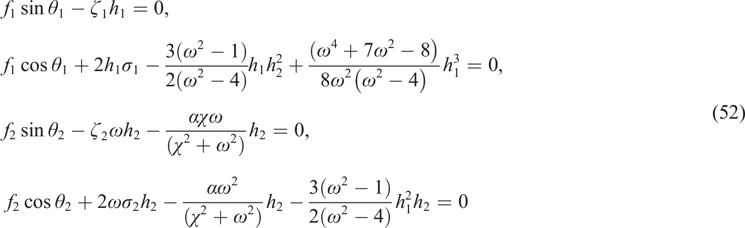
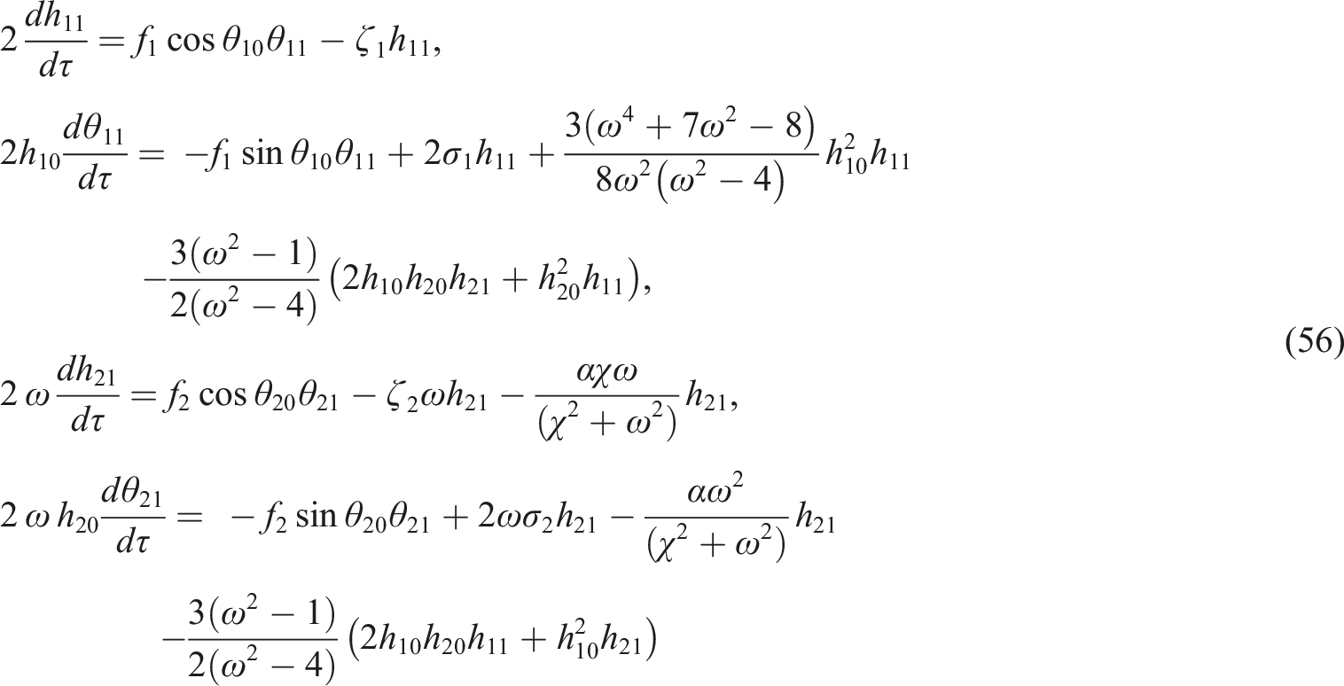
Substituting (42) and (43) into (22), (23), (25), and (26) and eliminating terms that produce the secular terms, we establish the conditions of solvability in the following forms:

- In accordance with the second-order of approximation

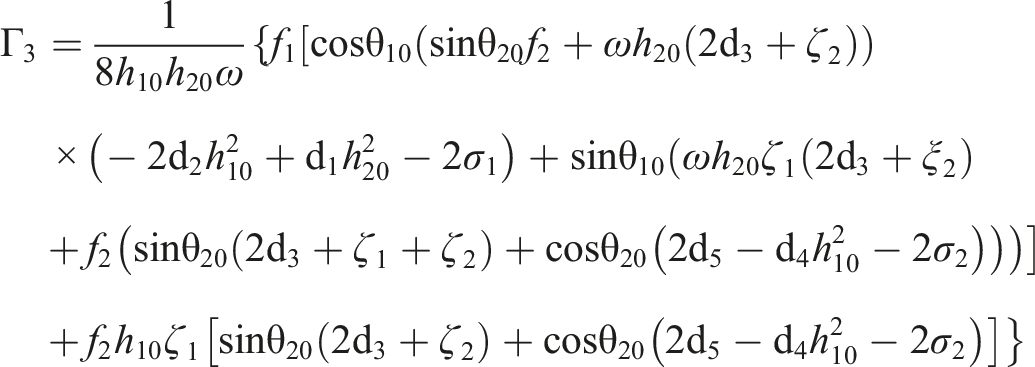
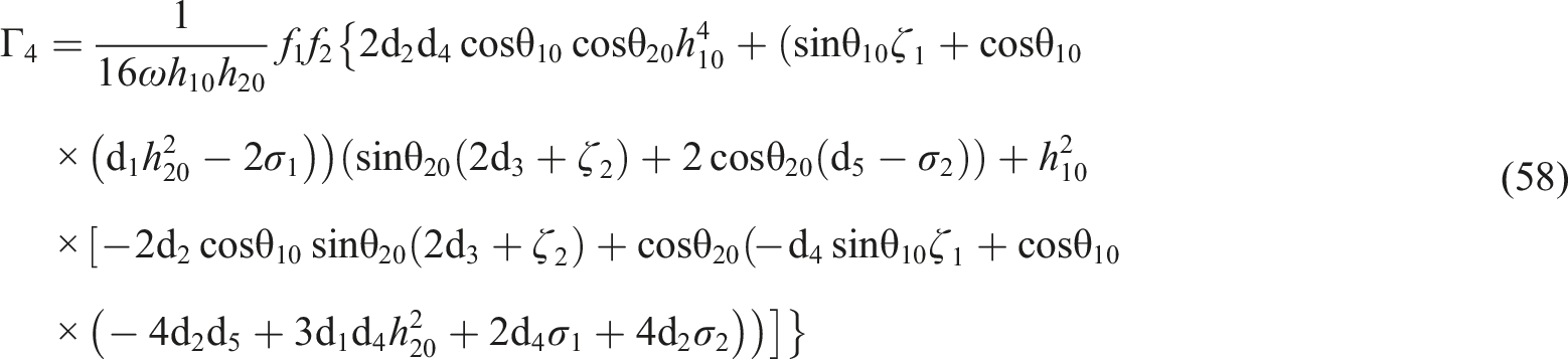
\frac{\partial Α_{1}}{\partial τ_{1}} = 0, \frac{\partial Α_{2}}{\partial τ_{1}} = 0, \frac{\partial B_{1}}{\partial τ_{1}} = 0 .

(44)

- In accordance with the third-order of approximation

\begin{array}{l} {\tilde{f}}_{1} e^{i τ_{1} {\tilde{σ}}_{1}} - 4 i \frac{\partial Α_{1}}{\partial τ_{2}} - 2 i {\tilde{ζ}}_{1} Α_{1} - \frac{12 (ω^{2} - 1)}{(ω^{2} - 4)} Α_{1} Α_{2} {\bar{Α}}_{2} + \frac{ω^{4} + 7 ω^{2} - 8}{ω^{2} (ω^{2} - 4)} Α_{1}^{2} {\bar{Α}}_{1} = 0, \\ {\tilde{f}}_{2} e^{i τ_{1} {\tilde{σ}}_{2}} - 4 i ω \frac{\partial Α_{2}}{\partial τ_{2}} - 2 i {\tilde{ζ}}_{2} ω Α_{2} - \frac{2 i \tilde{α} ω}{(χ + i ω)} Α_{2} - \frac{12 (ω^{2} - 1)}{(ω^{2} - 4)} Α_{1} {\bar{Α}}_{1} Α_{2} = 0. \\ \frac{\partial B_{1}}{\partial τ_{2}} - \frac{\tilde{α} χ B_{1}}{χ^{2} + ω^{2}} = 0. \end{array}

(45)

From the third equation of (45) and the conditions (44), we can obtain the expression of $B_{1}$ in the form

B_{1} = e^{(\frac{\tilde{α} χ}{χ^{2} + ω^{2}} τ_{2} + B_{2})}

(46)

where

B_{2}

is an unknown complex function of the higher slow time scales than

τ_{2}

Referring to the above solvability conditions (44) and (45), we can determine the functions $Α_{j} (j = 1,2)$ , which depend only on $τ_{2}$ . Therefore, we consider the polar forms $A_{j}$ according to the following

A_{j} = \frac{1}{2} {\tilde{h}}_{j} (τ_{2}) e^{i {\tilde{ψ}}_{j} (τ_{2})}, h_{j} = ε {\tilde{h}}_{j} (j = 1, 2) .

(47)

where

{\tilde{ψ}}_{j}

and

{\tilde{h}}_{j}

are real functions of the amplitudes and phases of the solutions

y

and

ϕ

, respectively.

Since $Α_{j}$ are dependent only on $τ_{2}$ , then their first-order derivatives will have the form

\frac{d A_{j}}{d τ} = ε^{2} \frac{\partial A_{j}}{\partial τ_{2}} (j = 1, 2)

(48)

Considering the previous formula (48), we convert PDE (45) to ordinary differential equations (ODEs) according to the following substitution of the modified phases

θ_{j} (τ_{2}) = τ_{1} {\tilde{σ}}_{j} - ψ_{j} (τ_{2}) j = (1,2)

(49)

Substituting (47)–(49) into (45) and then distinguishing the real portions and the imaginary ones, we obtain the desired autonomous system of PDE in the form

\begin{array}{l} 2 \frac{d h_{1}}{d τ} = f_{1} \sin θ_{1} - ζ_{1} h_{1}, \\ 2 h_{1} \frac{d θ_{1}}{d τ} = f_{1} \cos θ_{1} + 2 h_{1} σ_{1} - \frac{3 (ω^{2} - 1)}{2 (ω^{2} - 4)} h_{1} h_{2}^{2} + \frac{(ω^{4} + 7 ω^{2} - 8)}{8 ω^{2} (ω^{2} - 4)} h_{1}^{3}, \\ 2 ω \frac{d h_{2}}{d τ} = f_{2} \sin θ_{2} - ζ_{2} ω h_{2} - \frac{α χ ω}{(χ^{2} + ω^{2})} h_{2}, \\ 2 ω h_{2} \frac{d θ_{2}}{d τ} = f_{2} \cos θ_{2} + 2 ω σ_{2} h_{2} - \frac{α ω^{2}}{(χ^{2} + ω^{2})} h_{2} - \frac{3 (ω^{2} - 1)}{2 (ω^{2} - 4)} h_{1}^{2} h_{2} . \end{array}

(50)

Equations of the above system represent the equations of modulation for both modified phases $θ_{j} (j = 1,2)$ and amplitudes $h_{j}$ and, respectively, in which it consists of four ODEs from first order that can be obtained when two resonance cases occur at the same instance. The solutions of these equations are plotted for some selected values of the system’s parameters as in Figures 2–6 in accordance with the following data

c_{1} = 0.01 N .m .s/rad M_{0} = 0.005 N .m F_{0} = 0.08 N c_{2} = 0.02 N .s/m

m_{1} = (0.009, 0.010, 0.011) kg . a = 0.01 m Β = 1 Τ k = 8 kg {.s}^{- 2}

ℓ = (0.02, 0.03, 0.04) m b = 0.02 m Ω = 1 rad {.s}^{- 1} R = 100 Ω

w_{1} = (22.13, 18.07, 15.65) s^{- 1} σ_{1} = p_{1} - 1 Ω_{1} = 2 rad {.s}^{- 1} L_{coil} = 1 m

w_{2} = (29.81, 28.28, 26.97) s^{- 1} σ_{2} = p_{2} - ω Ω_{2} = 3 rad {.s}^{- 1} L_{ind} = 0.1 Η

Figure 2.

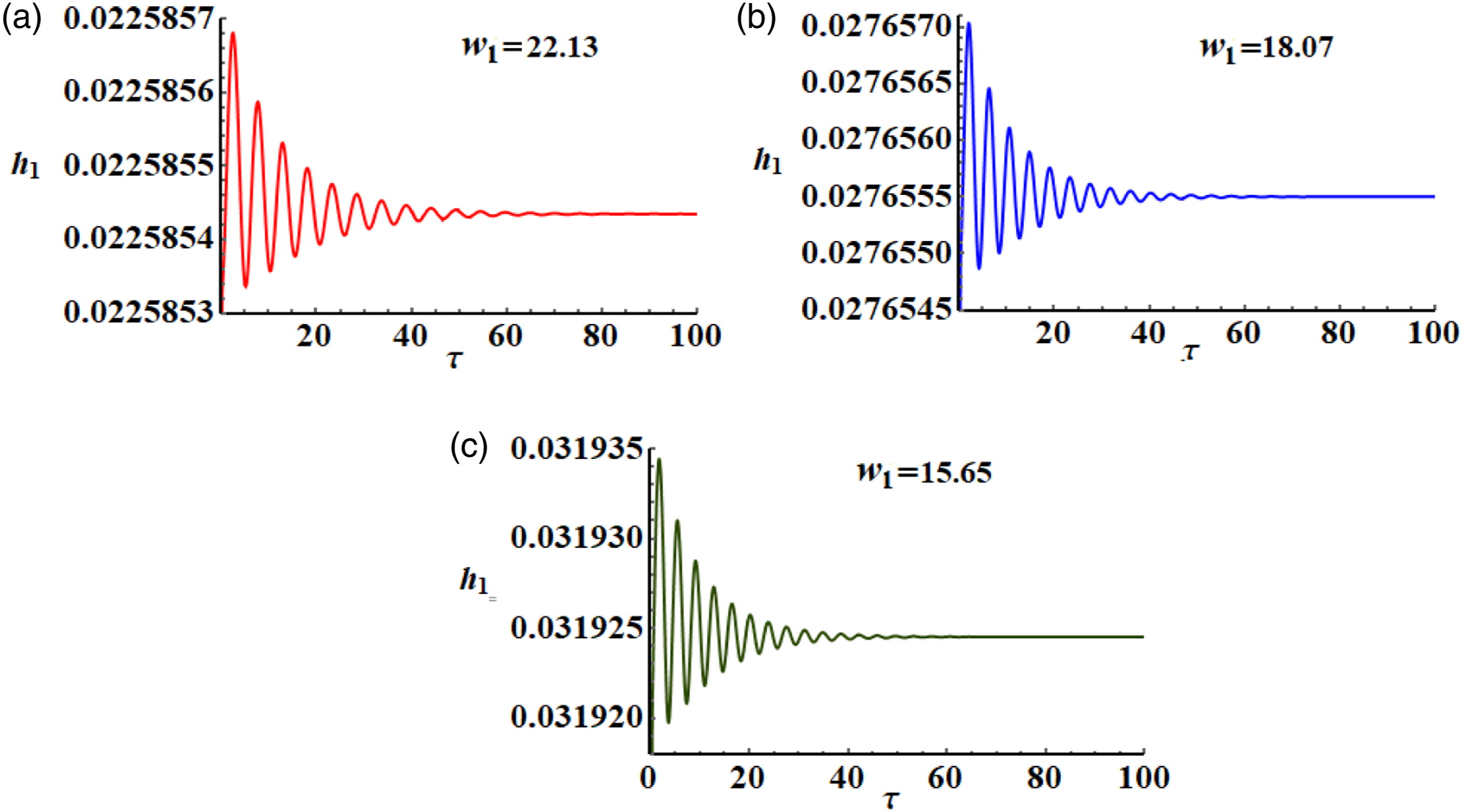
The amplitude’s time history of $h_{1}$ at $w_{1} = (22.13, 18.07, 15.65) s^{- 1}$ .

Figure 3.

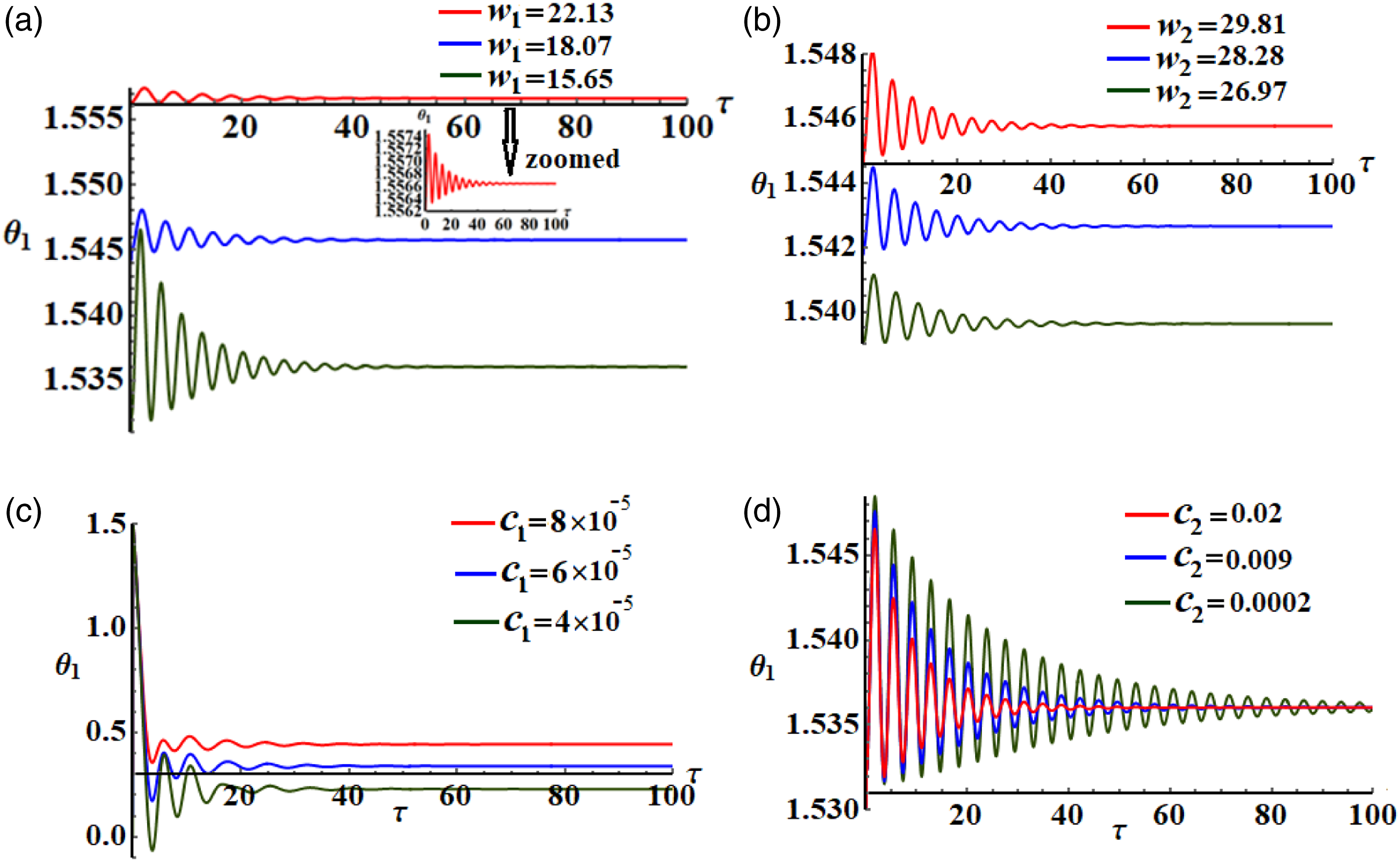
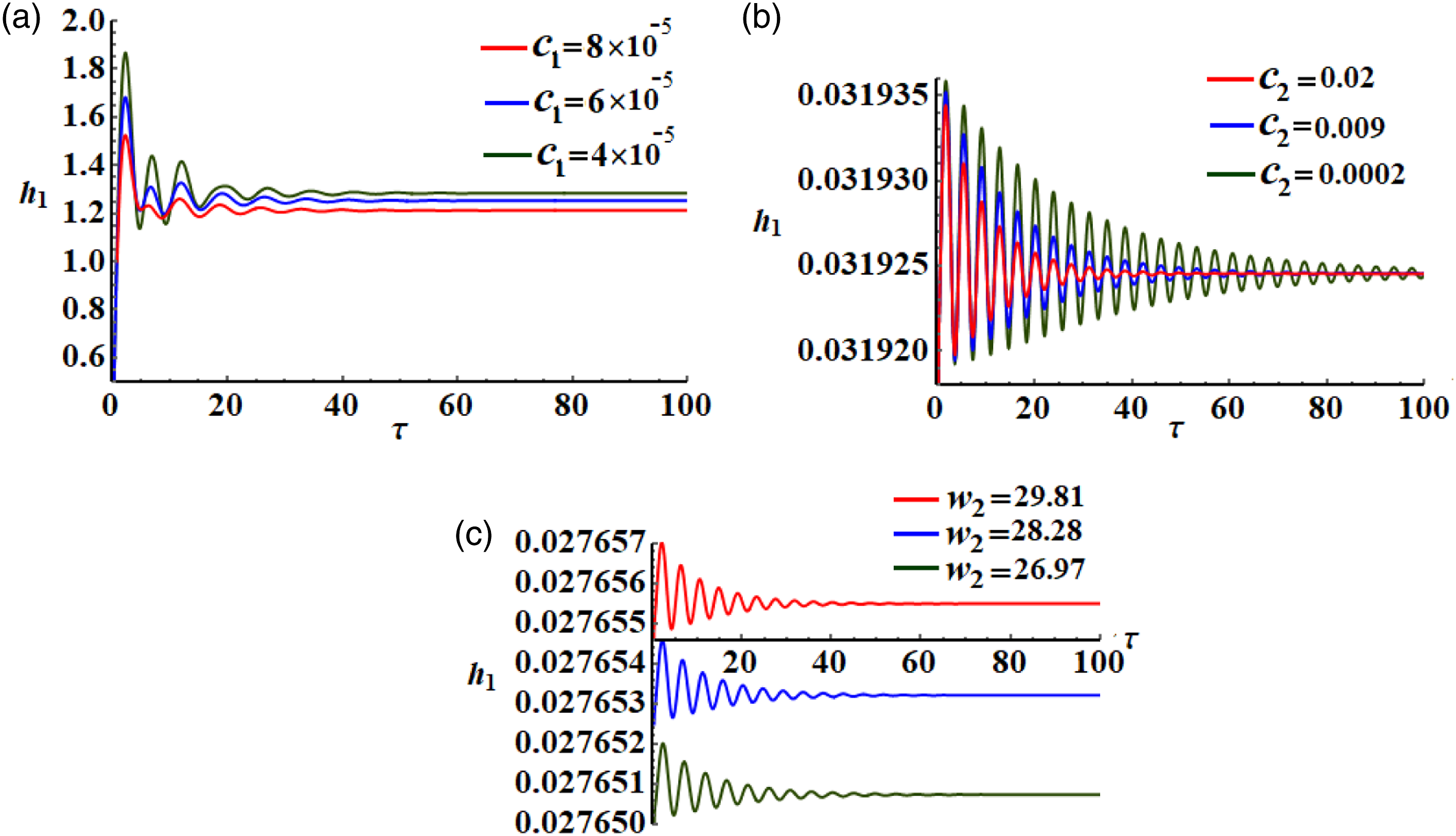
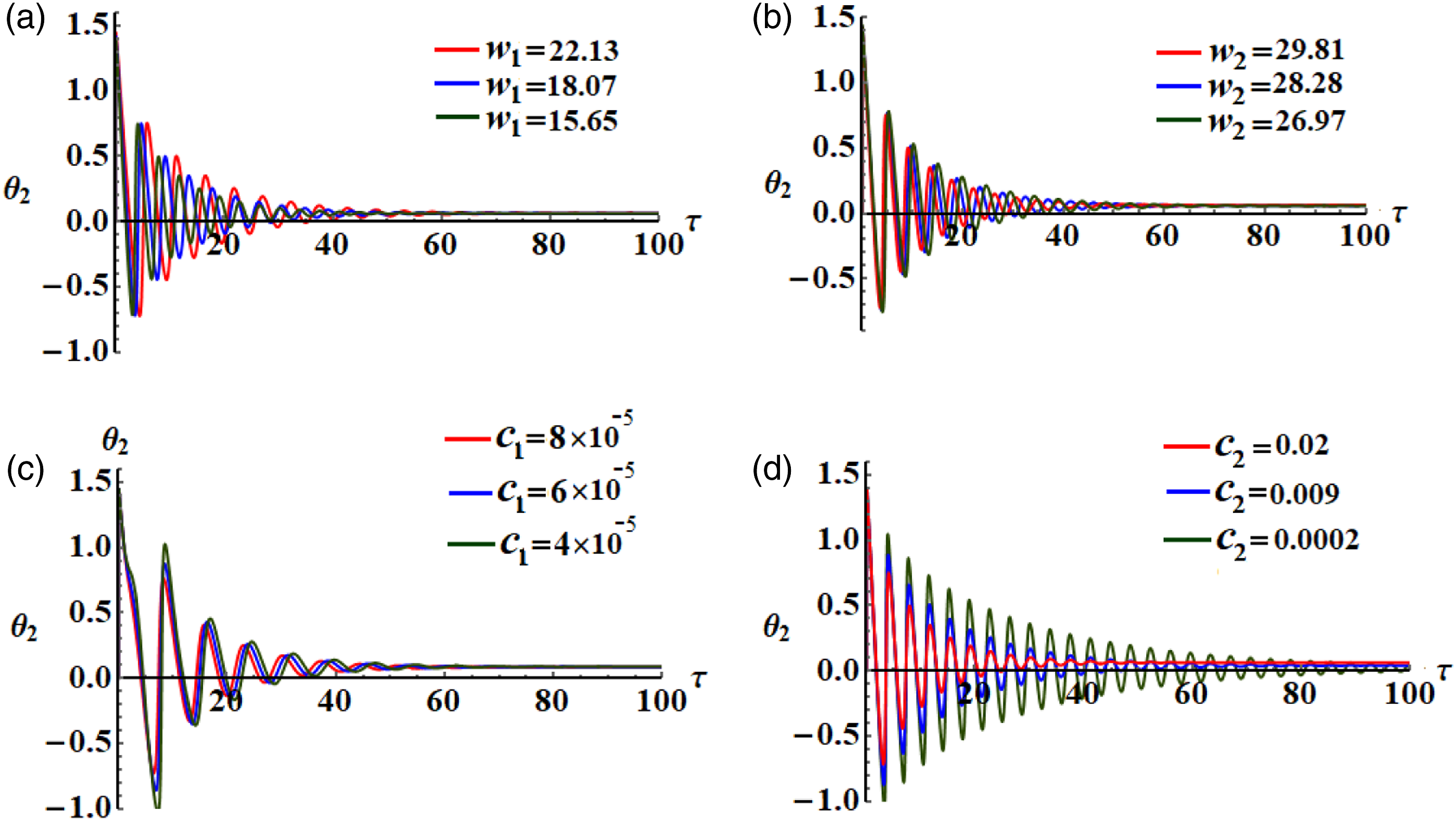
The change of the modified amplitude $h_{1}$ versus $τ$ at (a) $c_{1} = (8 \times 10^{- 5}, 6 \times 10^{- 5}, 4 \times 10^{- 5}) N .m .s/rad$ , (b) $c_{2} = (0.02, 0.009, 0.0002) N .s/m$ , and (c) $w_{2} = (29.81, 28.28, 26.97) s^{- 1}$ .

Figure 4.

The time history of $h_{2}$ at different values of $w_{j} (j = 1,2)$ and $c_{j} (j = 1,2)$ .

Figure 5.

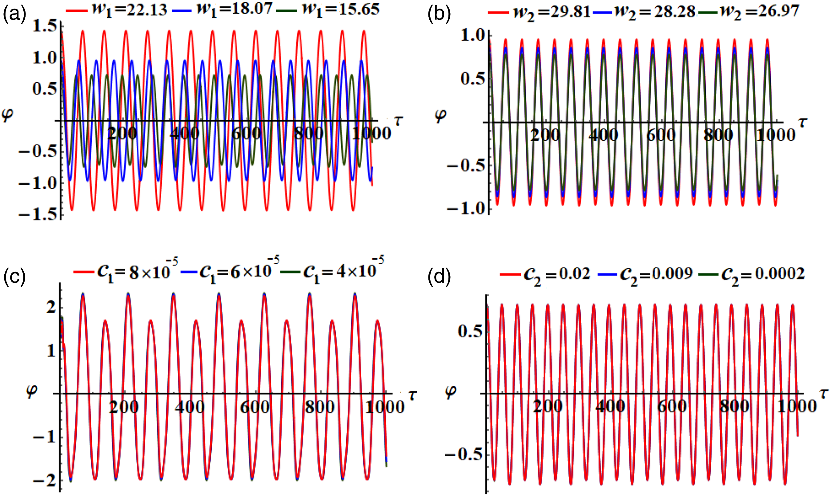
Modulation of the modified phase $θ_{1}$ versus time $τ$ at (a) $w_{1} = (22.13, 18.07, 15.65) s^{- 1}$ , (b) $w_{2} = (29.81, 28.28, 26.97) s^{- 1}$ , (c) $c_{1} = (8 \times 10^{- 5}, 6 \times 10^{- 5}, 4 \times 10^{- 5}) N .m .s/rad$ , and (d) $c_{2} = (0.02, 0.009, 0.0002) N .s/m$ .

Figure 6.

The time history of the modified phase $θ_{2}$ at selected values of $w_{j} (j = 1,2)$ and $c_{j} (j = 1,2)$ .

To investigate the importance of characteristic parameters on the dynamical system behavior, Figures 2–6 are plotted to display the transient responses of the modified amplitudes $h_{j}$ and the modified phases $θ_{j} (j = 1,2)$ at the specific values of $W_{j}$ . These values correspond to the normal length of the pendulum arm $ℓ$ , the mass $m_{1}$ of the magnet of the harvest, and the damping coefficient $c_{j} (j = 1,2)$ , as drawn in parts of these figures. Curves of these figures have decay forms when time $τ$ goes on, which points to the represented curves behave in a stable manner. Figure 2 sketches the variation of $h_{1}$ with time when $w_{1} = (22.13, 18.07, 15.65) s^{- 1}$ . When $w_{1}$ decreases, the vertical range of the wave describes that $h_{1}$ increases. A closer look at the parts of Figure 3 shows that they are calculated when $c_{1}, c_{2},$ and $w_{2}$ have the values $(8 \times 10^{- 5}, 6 \times 10^{- 5}, 4 \times 10^{- 5}) N .m .s/rad$ , $(0.02, 0.009, 0.0002) N .s/m$ , and $(29.81, 28.28, 26.97) s^{- 1}$ in which the variation of these parameters are shown in parts (a), (b), and (c), respectively. It is obvious to conclude that the increase of $c_{1}$ and $c_{2}$ values corresponding to the decreasing of the waves describes $h_{1}$ besides a decay behavior of these waves till the end of the time interval as seen in parts (a) and (b) of this figure, respectively. On the other hand, we can explore that the increasing of $w_{2}$ produces decreasing of the amplitudes of the waves, as seen in part (c). The reason of this variation is due to the first equation of the system (50).

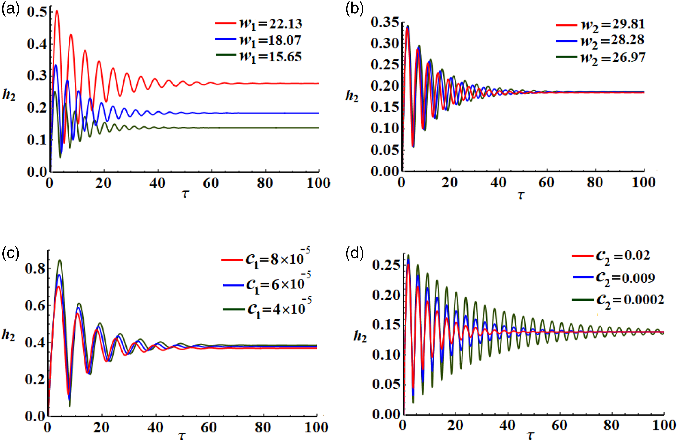
The inspection of the indicated curves of Figure 4 shows that the change happened in the amplitude $h_{2}$ with time $τ$ when $w_{1}, w_{2}, c_{1}$ , and $c_{2}$ have the above different selected values. In general, all plotted waves have a decaying manner with the values of these parameters, while the number of oscillations increases with the change of $w_{2}$ and $c_{2}$ than instead of $w_{1}$ and $c_{1}$ as seen in parts (a), (b), (c), and (d) of Figure 4. The comparison between curves of Figures 2 and 3 with the curves of Figure 4 explores that the variation of the waves describes $h_{2}$ has extremely high impulses than the other waves of $h_{1}$ except for the parts describing the variation of the values of $c_{1}$ . The main physical reason for these variations is due to the formal construction of the equations of system (50).

On the other side, Figures 5 and 6 introduce the variation of the modified phases $θ_{j} (j = 1,2)$ versus time $τ$ when $w_{j} (j = 1,2)$ and $c_{j} (j = 1,2)$ have distinctive values. It is concluded that the change of the values of $w_{j}$ has a minor impact on the waves describing the conduct of $θ_{2}$ as drawn in Figure 6(a) and (b), while this change becomes apparent sequentially with the other waves of $θ_{1}$ as shown in the parts (a), (b) of Figure 5. Parts (c) and (d) of the same figures portrait the effect of $c_{j}$ on the waves of $θ_{1}$ and $θ_{2}$ . The difference between the curves of these parts becomes closer with the variation of $θ_{2}$ than $θ_{1}$ , while the transient responses of the phases $θ_{j}$ behave like standing decay waves through the considered time interval and as obviously from Figures 5(d) and 6(d).

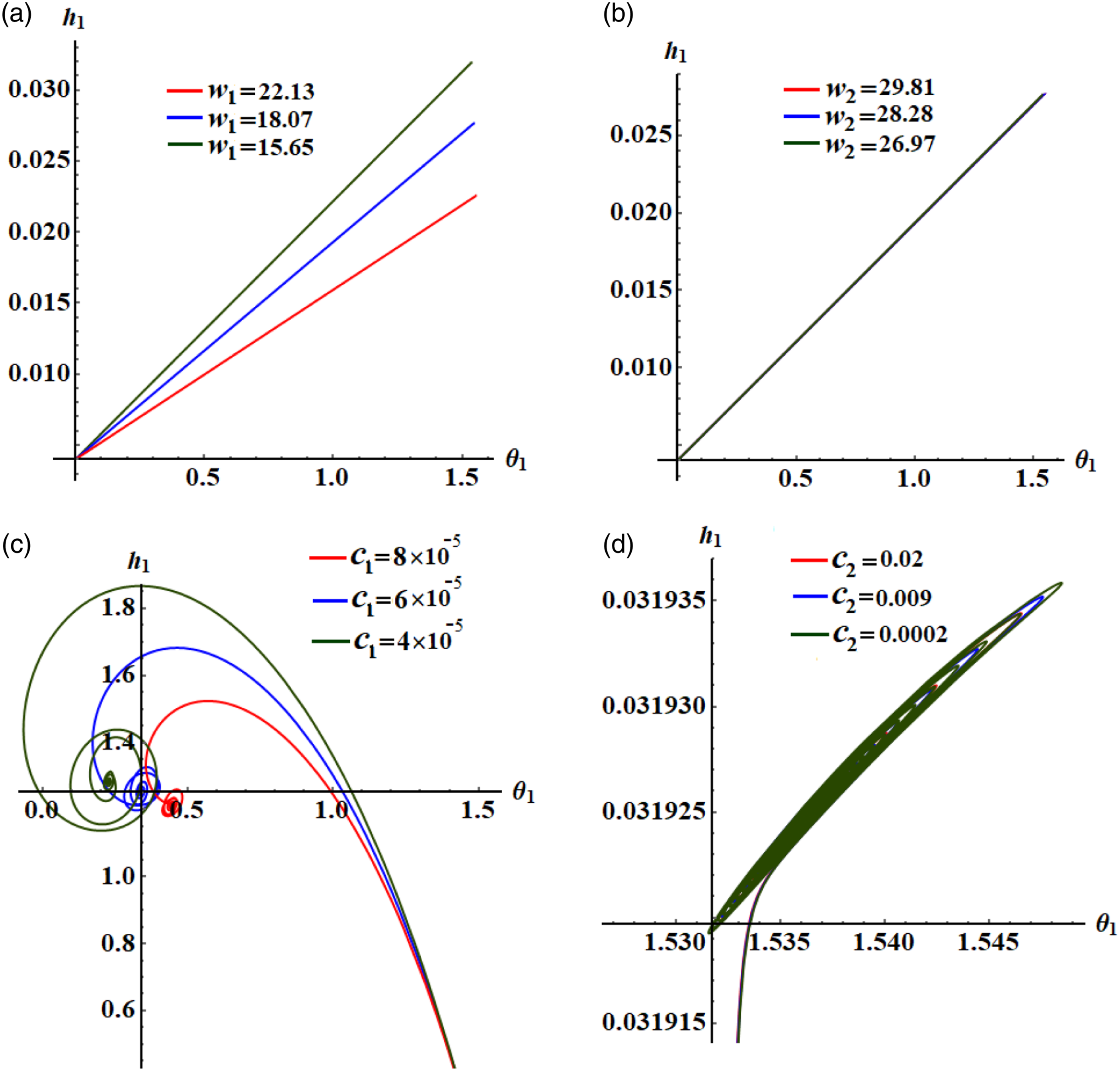
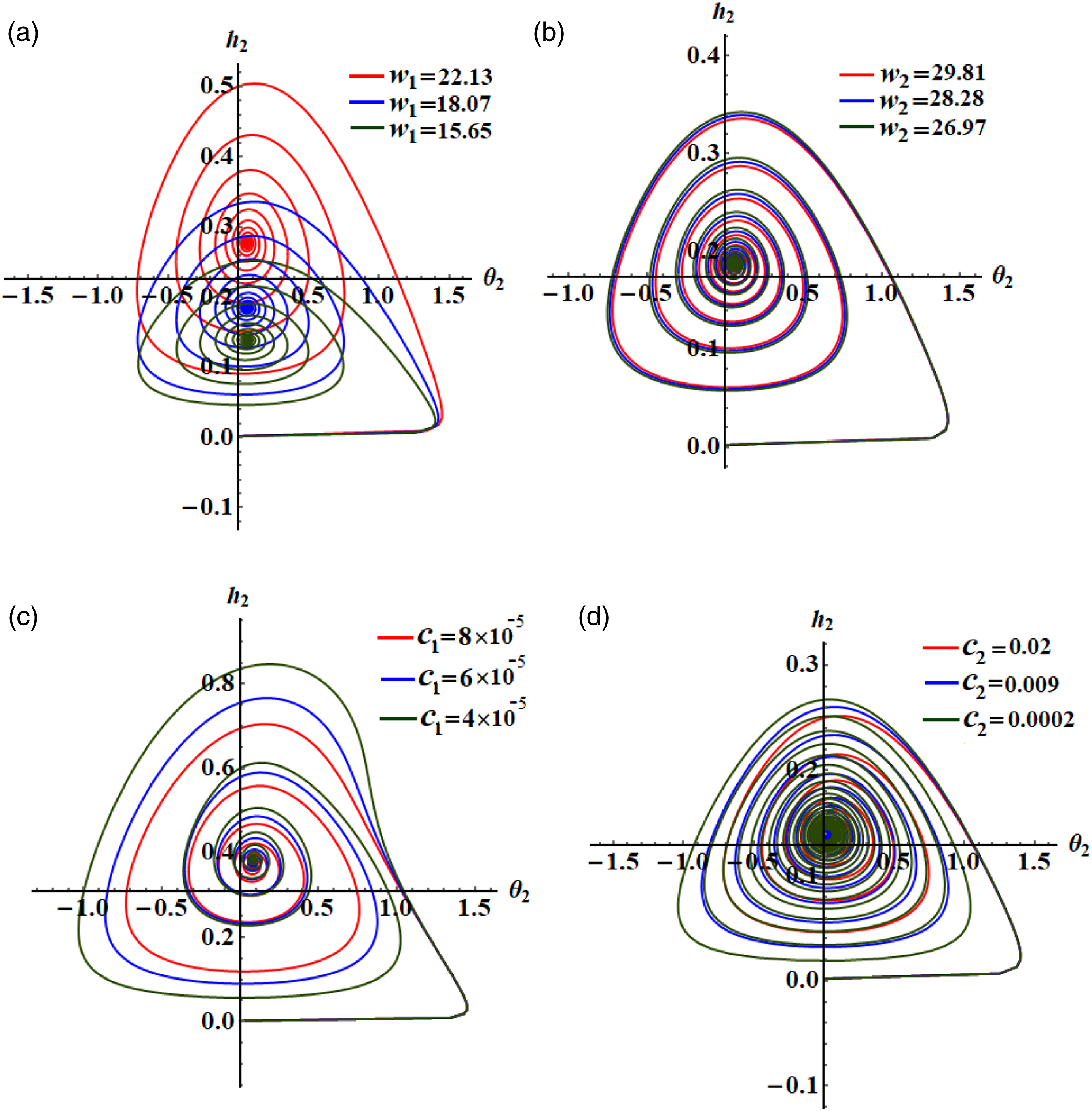
Figures 7 and 8 display the paths of amplitudes $h_{j} (j = 1,2)$ via the phases $θ_{j}$ at the same values of the previous data of $w_{j}$ and $c_{j}$ . It is notable that the projections of these paths on the space planes have the form of straight lines with the planes $h_{1} θ_{1}$ when $w_{j}$ have different values, as shown in parts (a) and (b) of Figure 7. The variation with $c_{j}$ produces curves that turn on themselves several times at the beginning of variation, while these curves coincide with each other at a certain point at the end of a time interval, as indicated in Figure 7(c) and (d). The plotted curves in Figure 8 displays circular spiral curves are produced when $w_{j}$ and $c_{j}$ have different values. In other words, the twisting curves converge on a single point, which describes the stable performances of the amplitude $h_{2}$ and the phase $θ_{2}$ .

Figure 7.

The phase plane $θ_{1} h_{1}$ at various values of $w_{j} (j = 1,2)$ and $c_{j}$ .

Figure 8.

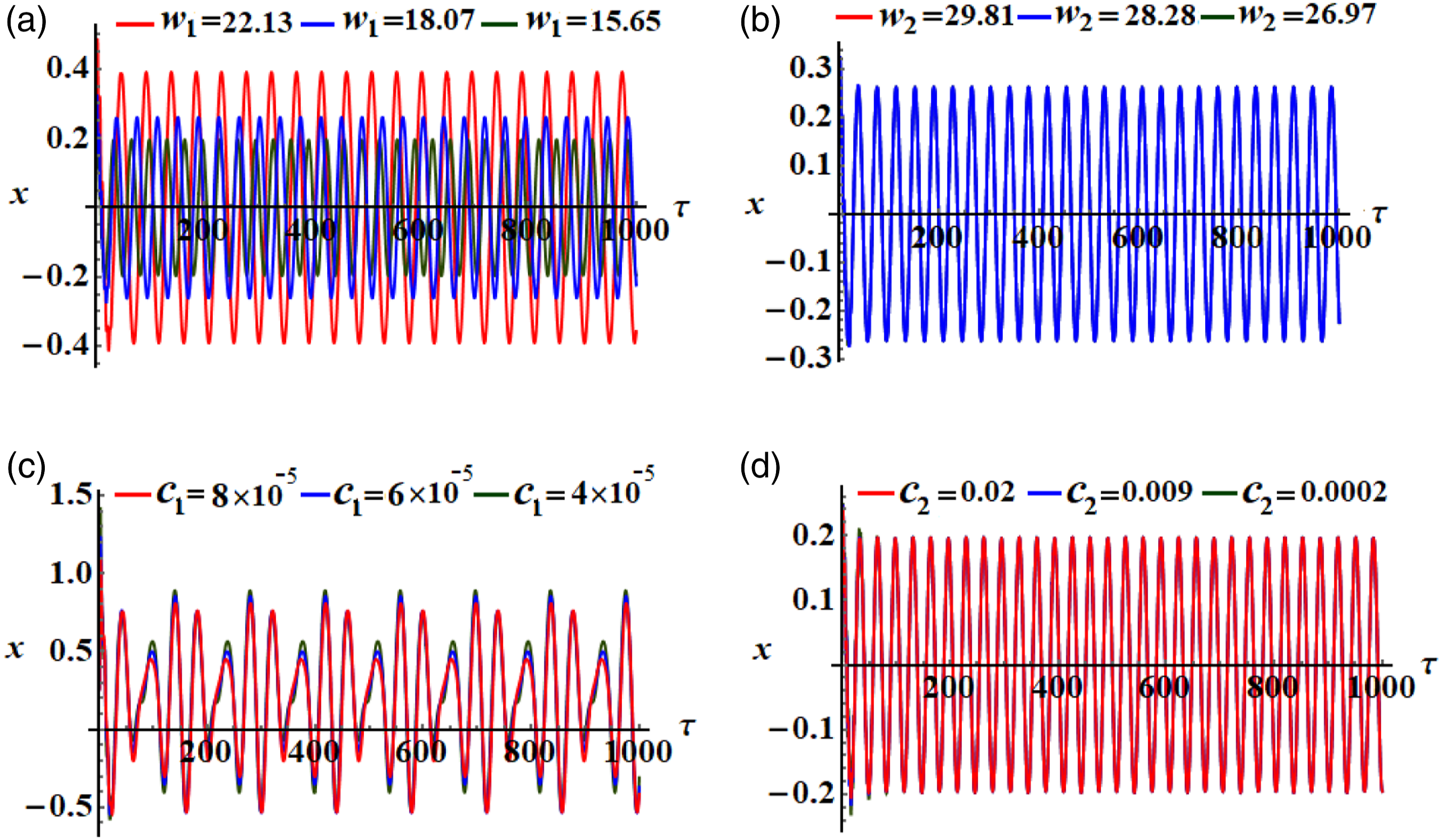
The phase plane $θ_{2} h_{2}$ is described for distinct values at (a) $w_{1} = (22.13, 18.07, 15.65) s^{- 1}$ , (b) $w_{2} = (29.81, 28.28, 26.97) s^{- 1}$ , (c) $c_{1} = (8 \times 10^{- 5}, 6 \times 10^{- 5}, 4 \times 10^{- 5}) N .m .s/rad$ , and (d) $c_{2} = (0.02, 0.009, 0.0002) N .s/m$ .

The drawn curves of Figures 9 and 10 explore the time-histories of solutions $φ$ and $x$ . The plotted curves have the forms of periodic waves, which assert the stability of these obtained solutions. A careful examination of these figures shows that when $w_{1}$ increases, the amplitude of the waves increases, and the oscillations’ number decreases, as seen in parts (a) of these figures. Alternatively, the amplitudes of the waves describing the behaviors of these solutions have a slight effect with the changing of $w_{2}$ and $c_{j}$ as noticed in parts (b), (c), and (d) of the same figures.

Figure 9.

The effectiveness of the physical parameters $w_{j} (j = 1,2)$ and $c_{j}$ is revealed on the solution $φ$ .

Figure 10.

The effect of variation of $w_{j} (j = 1,2)$ and $c_{j}$ on the solution $x$ .

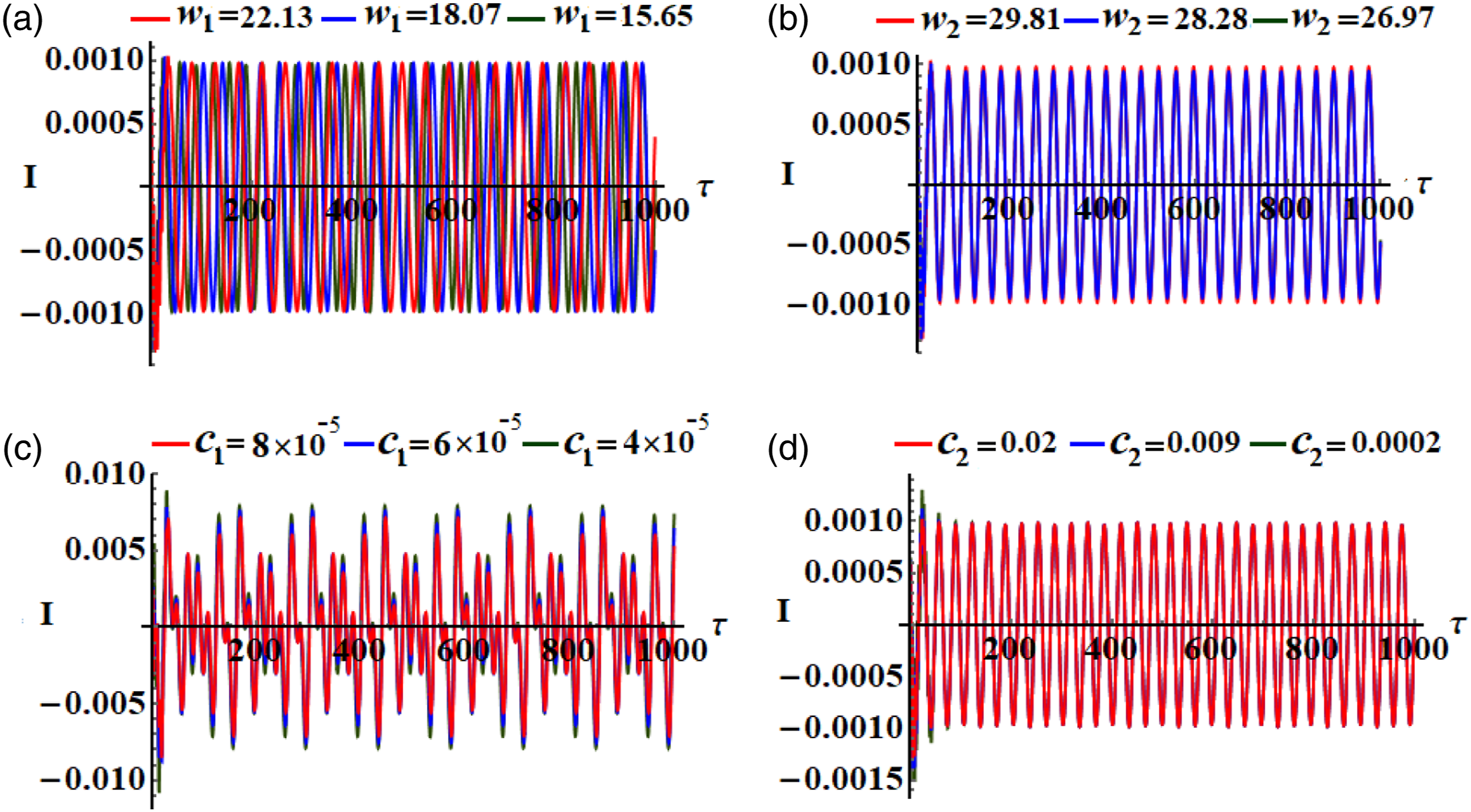
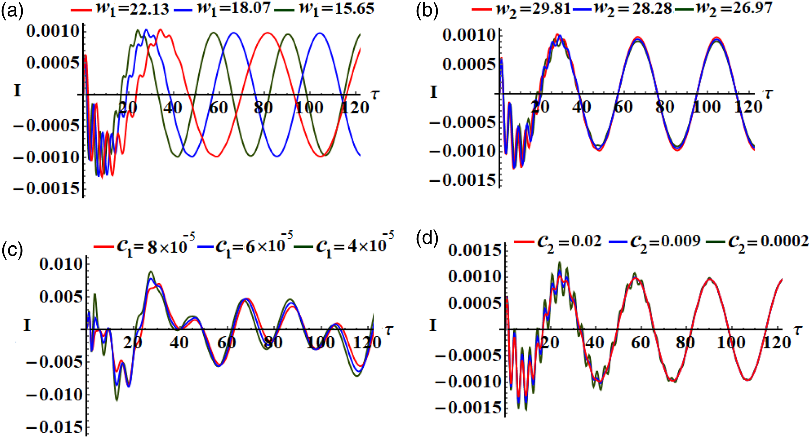
Figure 11 represents the small amplitudes of the current generated by the harvest circuit, leading to low levels of power at the output within milli-watts, which suit the sensor applications. Figure 12 focuses on the shape of the current wave $I$ , which reflects the presence of harmonic signals on the fundamental signals at the starting of the waves as transient current due to the RL circuit, and then the current behaves in a stationary form, which is required for uses.

Figure 11.

The time history of the current $I$ when $w_{j} (j = 1,2)$ and $c_{j}$ have different values.

Figure 12.

The influences of $w_{j} (j = 1,2)$ and $c_{j}$ on the behavior of the current $I$ at a small interval of time.

Steady-state solutions

This section aims to examine the model’s oscillations at the steady state, that is, when the oscillations of the transient process disappear due to the damping that occurs in the system. In such cases, equation (50) is of great significance in defining for this purpose, where the steady-state conditions correspond to the zero derivatives of the modified phases $θ_{j} (j = 1,2)$ and the amplitudes $h_{j}$ . Then, we can write

\frac{d h_{1}}{d t} = \frac{d h_{2}}{d t} = \frac{d θ_{1}}{d t} = \frac{d θ_{2}}{d t} = 0

(51)

Following these conditions, the following equations can be obtained

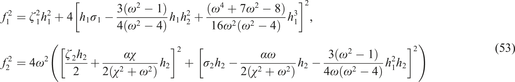
\begin{array}{l} f_{1} \sin θ_{1} - ζ_{1} h_{1} = 0, \\ f_{1} \cos θ_{1} + 2 h_{1} σ_{1} - \frac{3 (ω^{2} - 1)}{2 (ω^{2} - 4)} h_{1} h_{2}^{2} + \frac{(ω^{4} + 7 ω^{2} - 8)}{8 ω^{2} (ω^{2} - 4)} h_{1}^{3} = 0, \\ f_{2} \sin θ_{2} - ζ_{2} ω h_{2} - \frac{α χ ω}{(χ^{2} + ω^{2})} h_{2} = 0, \\ f_{2} \cos θ_{2} + 2 ω σ_{2} h_{2} - \frac{α ω^{2}}{(χ^{2} + ω^{2})} h_{2} - \frac{3 (ω^{2} - 1)}{2 (ω^{2} - 4)} h_{1}^{2} h_{2} = 0 \end{array}

(52)

At this end, it can be stated that the preceding system contains four algebraic equations in terms of $h_{j}$ and $θ_{j}$ . If we can remove $θ_{j}$ , we directly acquire the following two equations in terms of the amplitudes $h_{j}$ and the parameters of detuning $σ_{j}$

\begin{array}{l} f_{1}^{2} = ζ_{1}^{2} h_{1}^{2} + 4 {[h_{1} σ_{1} - \frac{3 (ω^{2} - 1)}{4 (ω^{2} - 4)} h_{1} h_{2}^{2} + \frac{(ω^{4} + 7 ω^{2} - 8)}{16 ω^{2} (ω^{2} - 4)} h_{1}^{3}]}^{2}, \\ f_{2}^{2} = 4 ω^{2} ({[\frac{ζ_{2} h_{2}}{2} + \frac{α χ}{2 (χ^{2} + ω^{2})} h_{2}]}^{2} + {[σ_{2} h_{2} - \frac{α ω}{2 (χ^{2} + ω^{2})} h_{2} - \frac{3 (ω^{2} - 1)}{4 ω (ω^{2} - 4)} h_{1}^{2} h_{2}]}^{2}) \end{array}

(53)

Moreover, the relationship of the amplitude–frequency of current has the form

z_{1} = \frac{ω h_{2}}{ε \sqrt{χ^{2} + ω^{2}}}

(54)

The steady-state vibrations are considered as important parts of the examination of the stability analysis of the considered system. To achieve such a case, we consider the performance of the system in a region very close to the fixed points. Therefore, the following expressions of $h_{j}$ and $θ_{j}$ are considered

\begin{array}{l} h_{j} = h_{j 0} + h_{j 1}, \\ θ_{j} = θ_{j 0} + θ_{j 1}, j = (1,2) \end{array}

(55)

Here, $h_{j 0}, θ_{j 0}$ are the solutions at the steady state, while $h_{j 1}, θ_{j 1}$ are the tiny perturbations comparing with $h_{j 0}, θ_{j 0}$ . Therefore, substituting (55) into (50) to obtain the following system

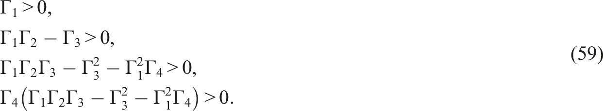
\begin{array}{l} 2 \frac{d h_{11}}{d τ} = f_{1} \cos θ_{10} θ_{11} - ζ_{1} h_{11}, \\ 2 h_{10} \frac{d θ_{11}}{d τ} = - f_{1} \sin θ_{10} θ_{11} + 2 σ_{1} h_{11} + \frac{3 (ω^{4} + 7 ω^{2} - 8)}{8 ω^{2} (ω^{2} - 4)} h_{10}^{2} h_{11} \\ - \frac{3 (ω^{2} - 1)}{2 (ω^{2} - 4)} (2 h_{10} h_{20} h_{21} + h_{20}^{2} h_{11}), \\ 2 ω \frac{d h_{21}}{d τ} = f_{2} \cos θ_{20} θ_{21} - ζ_{2} ω h_{21} - \frac{α χ ω}{(χ^{2} + ω^{2})} h_{21}, \\ 2 ω h_{20} \frac{d θ_{21}}{d τ} = - f_{2} \sin θ_{20} θ_{21} + 2 ω σ_{2} h_{21} - \frac{α ω^{2}}{(χ^{2} + ω^{2})} h_{21} \\ - \frac{3 (ω^{2} - 1)}{2 (ω^{2} - 4)} (2 h_{10} h_{20} h_{11} + h_{10}^{2} h_{21}) \end{array}

(56)

Since $h_{j 1}$ and $θ_{j 1}$ are unknown perturbed functions of both the amplitudes and the modified phases, respectively, then, we can write their solutions as a linear superposition of $ℏ_{s} e^{λ τ} (s = 1,2, ..., 4)$ where $λ$ and $ℏ_{s}$ are eigenvalues and constants, respectively. If the steady-state solutions $h_{j 0}$ and $θ_{j 0}$ are asymptotically stable, then the real partitions of the roots of the next characteristic equation of (56) should be negative

λ^{4} + Γ_{1} λ^{3} + Γ_{2} λ^{2} + Γ_{3} λ + Γ_{4} = 0

(57)

where

Γ_{s} (s = 1,2, ..., 4)

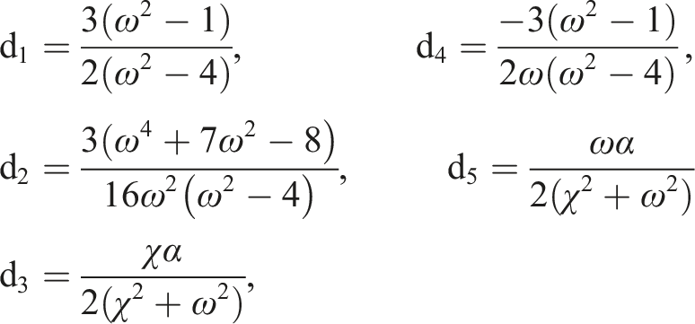
have the forms

\begin{array}{l} Γ_{1} = \frac{1}{2} (ζ_{1} + ζ_{2} + 2 d_{3} + \frac{f_{1} {sinθ}_{10}}{h_{10}} + \frac{f_{2} {sinθ}_{20}}{h_{20} ω}), \\ {\begin{cases} Γ_{2} = \frac{1}{4 ω h_{10} h_{20}} \sin θ_{20} f_{2} [\sin θ_{10} f_{1} + h_{10} (ζ_{1} + ζ_{2} \\ + 2 d_{3})] + ω h_{20} [h_{10} ζ_{1} (2 d_{3} + ζ_{2}) + f_{1} (\sin θ_{10} \\ \times (2 d_{3} + ζ_{1} + ζ_{2}) + \cos θ_{10} (- 2 d_{2} h_{10}^{2} + d_{1} h_{20}^{2} \\ - 2 σ_{1}))] - \cos θ_{20} f_{2} h_{10} (- 2 d_{5} + d_{4} h_{10}^{2} + 2 σ_{2}) \end{cases}} \end{array}

\begin{array}{l} Γ_{3} = \frac{1}{8 h_{10} h_{20} ω} {f_{1} [\cos θ_{10} (\sin θ_{20} f_{2} + ω h_{20} (2 d_{3} + ζ_{2})) \\ \times (- 2 d_{2} h_{10}^{2} + d_{1} h_{20}^{2} - 2 σ_{1}) + \sin θ_{10} (ω h_{20} ζ_{1} (2 d_{3} + ξ_{2}) \\ + f_{2} (\sin θ_{20} (2 d_{3} + ζ_{1} + ζ_{2}) + \cos θ_{20} (2 d_{5} - d_{4} h_{10}^{2} - 2 σ_{2})))] \\ + f_{2} h_{10} ζ_{1} [\sin θ_{20} (2 d_{3} + ζ_{2}) + \cos θ_{20} (2 d_{5} - d_{4} h_{10}^{2} - 2 σ_{2})]} \end{array}

\begin{array}{l} Γ_{4} = \frac{1}{16 ω h_{10} h_{20}} f_{1} f_{2} {2 d_{2} d_{4} \cos θ_{10} \cos θ_{20} h_{10}^{4} + (\sin θ_{10} ζ_{1} + \cos θ_{10} \\ \times (d_{1} h_{20}^{2} - 2 σ_{1})) (\sin θ_{20} (2 d_{3} + ζ_{2}) + 2 \cos θ_{20} (d_{5} - σ_{2})) + h_{10}^{2} \\ \times [- 2 d_{2} \cos θ_{10} \sin θ_{20} (2 d_{3} + ζ_{2}) + \cos θ_{20} (- d_{4} \sin θ_{10} ζ_{1} + \cos θ_{10} \\ \times (- 4 d_{2} d_{5} + 3 d_{1} d_{4} h_{20}^{2} + 2 d_{4} σ_{1} + 4 d_{2} σ_{2}))]} \end{array}

(58)

where

\begin{array}{l} d_{1} = \frac{3 (ω^{2} - 1)}{2 (ω^{2} - 4)}, d_{4} = \frac{- 3 (ω^{2} - 1)}{2 ω (ω^{2} - 4)}, \\ d_{2} = \frac{3 (ω^{4} + 7 ω^{2} - 8)}{16 ω^{2} (ω^{2} - 4)}, d_{5} = \frac{ω α}{2 (χ^{2} + ω^{2})} \\ d_{3} = \frac{χ α}{2 (χ^{2} + ω^{2})}, \end{array}

Now, we can write the basic conditions of stability which are in agreement with the Routh–Hurwitz principle²² for the specific steady-state solutions in the forms

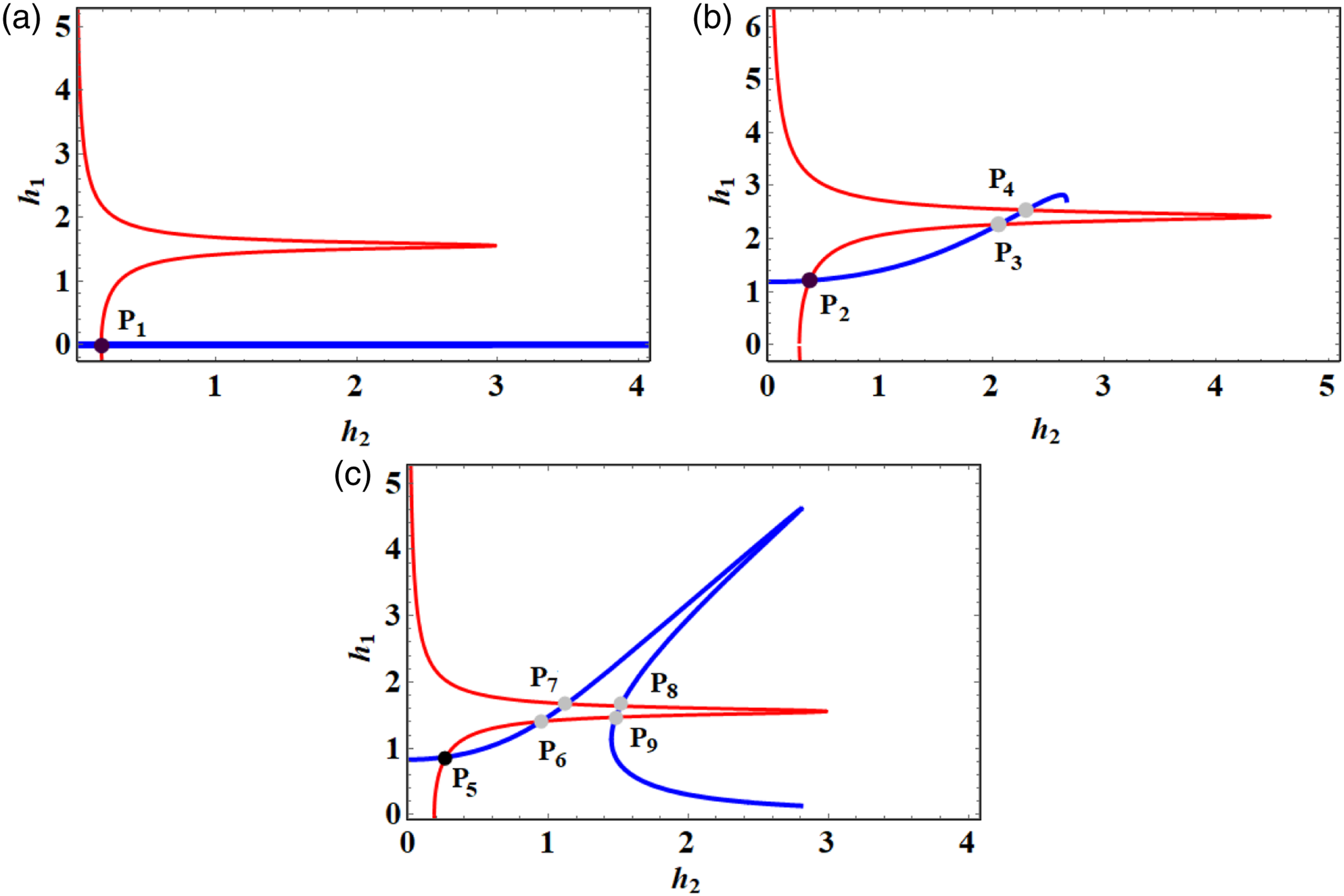
\begin{array}{l} Γ_{1} > 0, \\ Γ_{1} Γ_{2} - Γ_{3} > 0, \\ Γ_{1} Γ_{2} Γ_{3} - Γ_{3}^{2} - Γ_{1}^{2} Γ_{4} > 0, \\ Γ_{4} (Γ_{1} Γ_{2} Γ_{3} - Γ_{3}^{2} - Γ_{1}^{2} Γ_{4}) > 0. \end{array}

(59)

A closer look at the curves of Figure 13 explores the steady-state solutions of the amplitudes $h_{1}$ and $h_{2}$ when $σ_{1} = p_{1} - 1, σ_{2} = p_{2} - ω,$ in the framework of equations of system (53) with the aid of Routh–Hurwitz conditions (59). The blue curves represent the locus of the roots of the first equation of (53), while the red curves indicate the solutions of the second equation of (53). The intersection points of these curves identify the solutions of both equations of (53). The axial amplitudes and adjusting vibration in the steady-state are determined definitively by these points. In addition, oscillations at the steady-state might be stable or unstable. The stable fixed points are marked by small black circles, while the unstable ones are marked by small gray circles. Curves of Figure 13(a) are calculated when $c_{1} = 0.01, c_{2} = 0.02, ℓ = 0.03$ , and $m = 0.009$ to obtain one stable fixed point at $P_{1}$ (see Table 1). Three fixed points $P_{S} (s = 2,3,4)$ in Table 1 are obtained in Figure 13(b) when $c_{1} = 8 \times 10^{- 5}, c_{2} = 0.02, ℓ = 0.04$ , and $m = 0.009$ , in which one of them is a stable fixed point and the others are unstable. Finally, to provide a better view about the fixed points, let us shed light on Figure 13(c), which has been sketched at $c_{1} = 6 \times 10^{- 5}, c_{2} = 0.02, ℓ = 0.03$ , and $m = 0.009$ . Five fixed points $P_{k} (k = 5,6, ..., 9)$ are achieved (see Table 1) which are classified into one stable fixed point, and the others are found unstable.

Figure 13.

The intersection of the amplitudes $h_{1}$ and $h_{2}$ to obtain the fixed points.

Table 1.

The fixed points $P_{e} (e = 1,2,3, ..., 9)$ .

Fixed points	Coordinates	Kind of fixed points
$P_{1}$	$(0.1888, 0.0057)$	Stable
$P_{2}$	$(0.380, 1.208)$	Stable
$P_{3}$	$(2.0554, 2.2506)$	Unstable
$P_{4}$	$(2.310, 2.549)$	Unstable
$P_{5}$	$(0.2698, 0.8689)$	Stable
$P_{6}$	$(0.9486, 1.4069)$	Unstable
$P_{7}$	$(1.1268, 1.6758)$	Unstable
$P_{8}$	$(1.4747, 1.4965)$	Unstable
$P_{9}$	$(1.5086, 1.640)$	Unstable

The analysis of stability

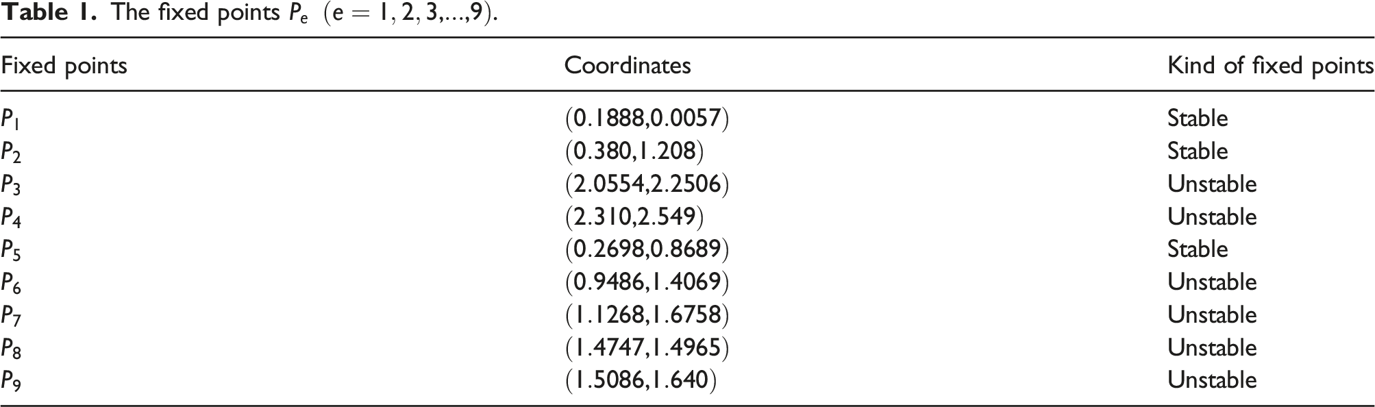
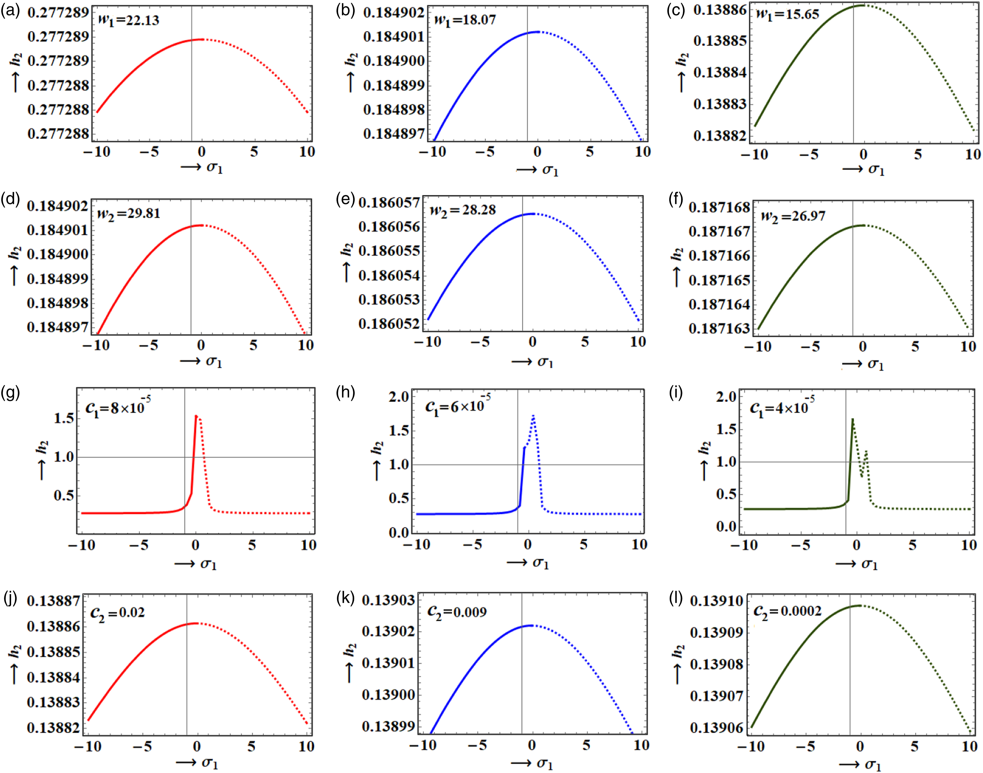
In this section, the non-linear stability approach is used to analyze the stability of the investigated system, in which the stability parameters are carried out as well as the system’s simulation. The detuning parameters $σ_{j} (j = 1,2)$ , the frequency amplitudes $w_{j}$ , and the damping coefficient $c_{j} (j = 1,2)$ play an important role, among the most important parameters, in the stabilization process. The stability diagrams are plotted for system (56), taking into account the selected values of these parameters. The modified amplitudes $h_{j}$ are plotted for various parametrical regions, in which its characteristics are submitted via the phase plane paths. The possible steady-state fixed points are sketched in Figures 14 and 15 with the varying values of $σ_{1}$ , where the range of the fixed points is $- 10 \leq σ_{1} \leq 10$ . It is observed from Figure 14(a) that at $w_{1} = 15.65$ , the range of stable fixed points is $- 10 \leq σ_{1} \leq - 0.1$ and the unstable one is satisfied in the area $- 0.1 < σ_{1} \leq 10$ . Moreover, the stable and unstable areas of fixed points at $w_{1} (= 22.13, 18.07)$ are $- 10 \leq σ_{1} \leq 0$ and $0 < σ_{1} \leq 10$ , respectively. The solid and the dashed curves denote the ranges of stable and unstable fixed points, respectively.

Figure 14.

The frequency response of $h_{1}$ via $σ_{1}$ at $σ_{2} = p_{2} - ω$ when (a) $w_{1} = (22.13, 18.07, 15.65) s^{- 1}$ , (b) $w_{2} = (29.81, 28.28, 26.97) s^{- 1}$ , (c) $c_{1} = (8 \times 10^{- 5}, 6 \times 10^{- 5}, 4 \times 10^{- 5}) N .m .s/rad$ , and (d) $c_{2} = (0.02, 0.009, 0.0002) N .s/m$ .

Figure 15.

Research on the variation of modified amplitude $h_{2}$ with the detuning parameter $σ_{1}$ at $σ_{2} = p_{2} - ω$ .

It should be noticed from Figure 14(b) that the possible fixed points are stable in the range $- 10 \leq σ_{1} \leq 0$ while they lose their stabilities in the area $0 < σ_{1} \leq 10$ . It is observed from Figure 14(c) that the area of stable fixed points at $c_{1} = 8 \times 10^{- 5}$ is $- 10 \leq σ_{1} \leq 0$ while the unstable one lies in the range $0 < σ_{1} \leq 10$ with one critical fixed point, which is the point between two areas. In the same context, we found two peaks at $c_{1} = (6 \times 10^{- 5}, 4 \times 10^{- 5}) N . m . s / r a d$ , in which the stable and unstable areas are $- 10 \leq σ_{1} \leq - 0.4$ and $- 0.4 < σ_{1} \leq 10$ , respectively. Finally, the curves of Figure 14(d) reveal that we have only one critical fixed point at $c_{2} = (0.02, 0.009, 0.0002) N . s / m$ with stable and unstable ranges $- 10 \leq σ_{1} \leq - 0.1$ and $- 0.1 < σ_{1} \leq 10$ , respectively. Based on the preceding presented analysis of Figure 14, we conclude that the amplitude $h_{2}$ via $σ_{1}$ has the same areas of stability and instability as seen in parts of Figure 15. The connection points between these curves characterize the critical values of the celebrity wave at which transcritical bifurcation is done due to one fixed point.

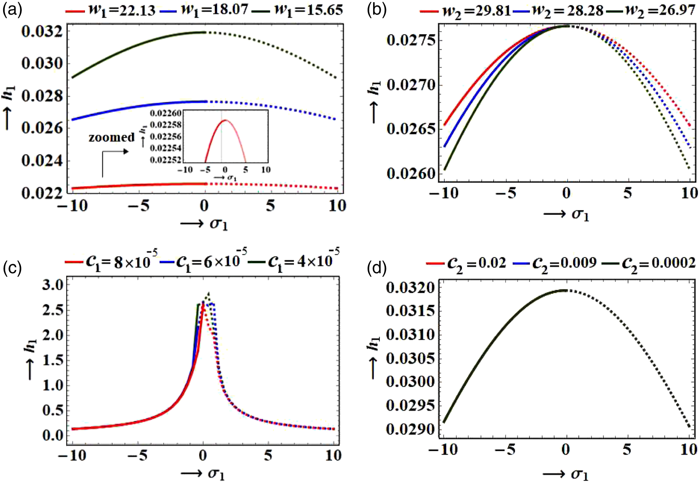
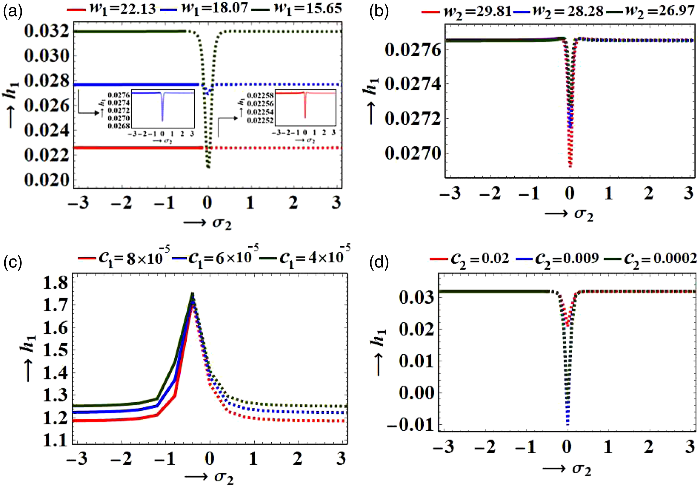
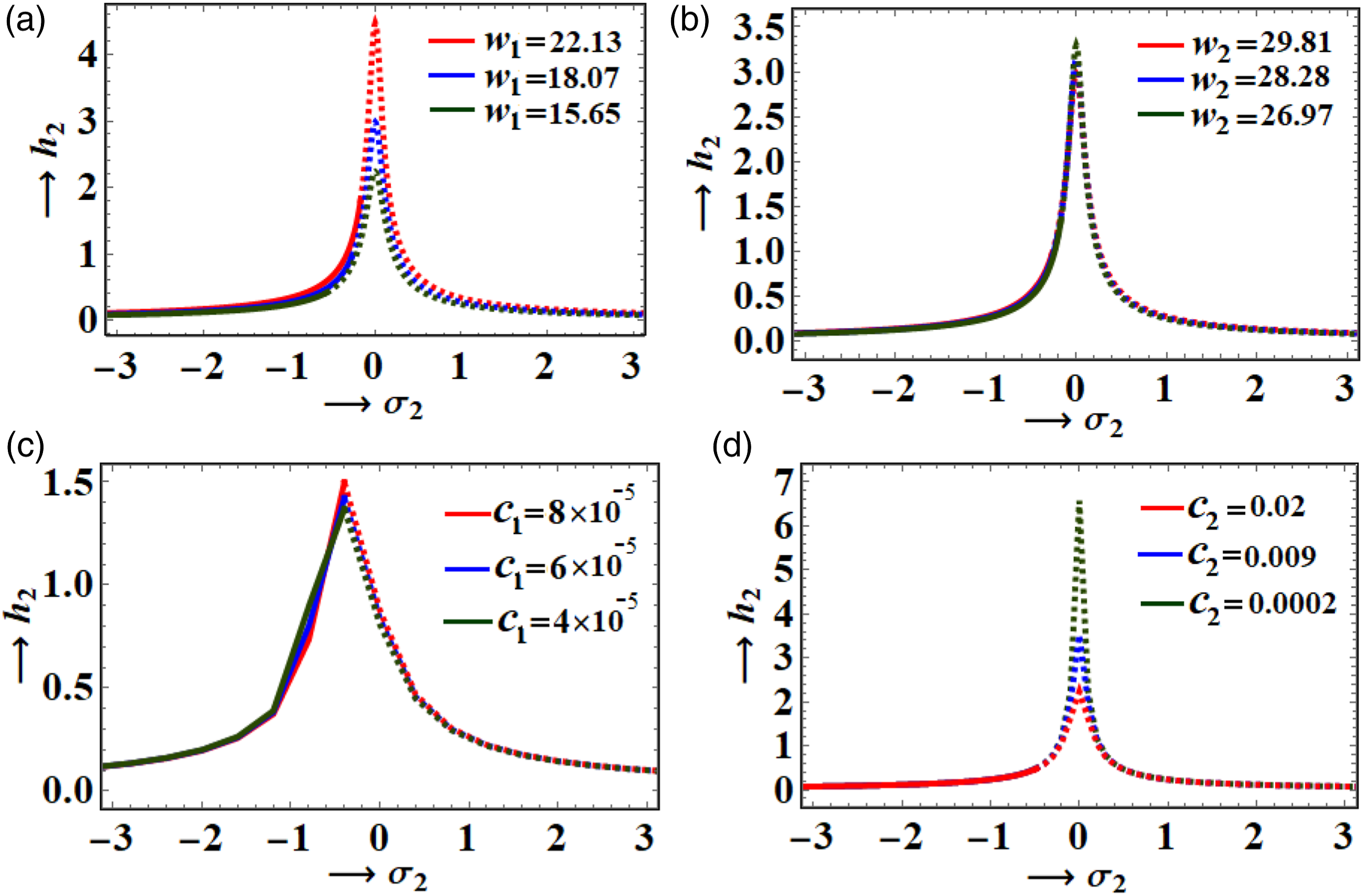
Figures 16 and 17 display the frequency response variation of $h_{j} (j = 1,2)$ via the detuning parameter $σ_{2}$ for different values of $w_{j}$ and $c_{j}$ through the range $- 3 \leq σ_{2} \leq 3$ at $σ_{1} = p_{1} - 1$ . The aim of the graphs is to generate the results of Figure 16, to examine the influence of $w_{j}$ and $c_{j}$ on the frequency response of $h_{1}$ versus $σ_{2}$ . Each curve has only one critical fixed point separated between the stable areas and unstable at $w_{1} (= 22.13, 18.07, 15.65) s^{- 1}$ as shown in part (a) of Figure 16. It is found that at $w_{1} = 22.13$ , the stable and unstable areas are $- 3 \leq σ_{2} \leq - 0.17$ and $- 0.17 < σ_{2} \leq 3$ , respectively, while at $w_{1} = 18.07$ , the stable and unstable areas are $- 3 \leq σ_{2} \leq - 0.27$ and $- 0.27 < σ_{2} \leq 3$ . Later, at $w_{1} = 15.65$ , one observes that the stable and unstable areas will be $- 3 \leq σ_{2} \leq - 0.57$ and $- 0.57 < σ_{2} \leq 3$ , respectively.

Figure 16.

The frequency response of $h_{1}$ versus $σ_{2}$ at $σ_{1} = p_{1} - 1$ when (a) $w_{1} = (22.13, 18.07, 15.65) s^{- 1}$ , (b) $w_{2} = (29.81, 28.28, 26.97) s^{- 1}$ , (c) $c_{1} = (8 \times 10^{- 5}, 6 \times 10^{- 5}, 4 \times 10^{- 5}) N .m .s/rad$ , and (d) $c_{2} = (0.02, 0.009, 0.0002) N .s/m$ .

Figure 17.

The variation of the modified amplitude $h_{2}$ versus the detuning parameter $σ_{2}$ at $σ_{1} = p_{1} - 1$ .

It is remarked from the curves of Figure 16(b) that there exists only one critical point and one peak when $w_{2} (= 29.81, 28.28, 26.97) s^{- 1}$ in which the stability and instability areas are found in the ranges $- 3 \leq σ_{2} \leq - 0.27,$ $- 3 < σ_{2} \leq - 0.21,$ $- 3 \leq σ_{2} \leq - 0.17,$ and $- 0.27 < σ_{2} \leq 3,$ $- 0.21 < σ_{2} \leq 3,$ $- 0.17 < σ_{2} \leq 3$ , respectively. Here, we can deduce that when $w_{2}$ increases, the peaks are slightly shifted down, as seen in Figure 16(b). The reason goes back to the realization of the Routh–Hurwitz conditions during the investigated range and to the equations of modulation (56).

The inspection of the curves displayed in Figure 16(c) shows that there is only one critical fixed point at $c_{1} = (8 \times 10^{- 5}, 6 \times 10^{- 5}, 4 \times 10^{- 5}) N .m .s/rad$ besides several peaks on these curves, in which the stable and unstable areas lie in the ranges $- 3 \leq σ_{2} \leq - 0.4$ and $- 0.4 < σ_{2} \leq 3$ , respectively. On the other hand, at $c_{2} (= 0.02, 0.009, 0.0002) N .s/m$ , the stable and unstable areas are found in the ranges $- 3 \leq σ_{2} \leq - 0.5$ and $- 0.5 < σ_{2} \leq 3$ , respectively. The same observations can also be applied to the corresponding parts of Figure 17.

Conclusion

The vibration reduction and the energy harvesting of a spring-pendulum of a novel dynamical system are investigated. The structure of the pendulum is adjusted using an independent electromagnetic harvesting device. The harvesting is based on a magnet in an oscillating coil. The harvester’s energy gathering, as well as its vibration mitigation performance, has been improved. Lagrange’s equations are applied to derive the EOM of this system, considering the influence of external forces and moments. Precise standardization of the approximate solutions is obtained using MSM. All secular terms are averted to acquire the solvability requirements and the modulation equations in light of the examination of the external resonance condition. The stability conditions are gained utilizing the Routh–Hurwitz conditions, in which the stability and instability regions are plotted and analyzed according to the determination of stable or unstable fixed points. The temporal histories of the modified phases and amplitudes generalized coordinates, frequency responses curves, and the stability and instability areas are drawn to expose the impact of the various parameters on the attitude of the studied system, in which the system displays transcritical bifurcations at certain values of $σ_{j}$ . The relevance of this work lies in its current uses in the control sensors.

Data availability statement

As no datasets were generated or processed during the current study, data sharing was not applicable to this paper.

Footnotes

Declaration of conflicting interests

The author(s) declared no potential conflicts of interest with respect to the research, authorship, and/or publication of this article.

Funding

The author(s) disclosed receipt of the following financial support for the research, authorship, and/or publication of this article: This study is supported by Shaanxi Province Educational Science Planning Project (SGH20Q207).

ORCID iDs

Chun-Hui He

Dan Tian

Tarek S Amer

Abdallah A Galal

References

Nath

Debnath

Choudhury

. Methods for improving the seismic performance of structures: a review, IOP Conf Ser Mater Sci Eng 2018; 377(1): 012141.

Den Hartog

. Mechanical vibrations. Courier Corporation, 1985.

Gong

Peng

Xuan

, et al. A pendulum-like tuned vibration absorber and its application to a multi-mode system. J Mech Sci Technol 2012; 26(11): 3411–3422.

Muralt

. Ferroelectric thin films for micro-sensors and actuators: a review. J Micromech Microeng 2000; 10(2): 136–146.

Zhou

Liao

. Analysis and design of a self-powered piezoelectric microaccelerometer. Proc SPIE 2005; 5763: 233–240.

Koeneman

Busch-Vishniac

Wood

K L

. Feasibility of micro power supplies for MEMS. J Microelectromechanical Syst 1997; 6(4): 355–362.

Paradiso

Starner

. Energy scavenging for mobile and wireless electronics. IEEE Pervasive Comput 2005; 4(1): 18–27.

Mizuno

Chetwynd

. Investigation of a resonance microgenerator. J Micromech Microeng 2003; 13(2): 209–216.

Mitcheson

Yeatman

Rao

, et al. Energy harvesting from human and machine motion for wireless electronic devices. Proc IEEE 2008; 96(9): 1457–1486.

10.

Naruse

Matsubara

Mabuchi

, et al. Electrostatic micro power generation from low-frequency vibration such as human motion. J Micromech Microeng 2009; 19(9): 094002.

11.

. Low-frequency piezoelectric energy harvesting prototype suitable for the MEMS implementation. Microelectronics J 2011; 42(2): 277–282.

12.

Galchev

Aktakka

Kim

, et al. A piezoelectric frequency-increased power generator for scavenging low-frequency ambient vibration. Proc MEMS Hong Kong 2010: 1203–1206.

13.

Nia

Zawawi

NAWA

Singh

BSM

. A review of walking energy harvesting using piezoelectric materials. IOP Conf Ser Mater Sci Eng 2017; 291(1): 012026.

14.

Liu

Zhang

, et al. Thermal oscillation arising in a heat shock of a porous hierarchy and its application. Facta Univ Ser Mech Eng 2021. DOI: 10.22190/FUME210317054L.

15.

El-Dib

. Multiple scales homotopy perturbation method for nonlinear oscillators. Nonlinear Sci Lett A 2017; 8(4): 352–364.

16.

Liu

, et al. Passive atmospheric water harvesting utilizing an ancient Chinese ink slab and its possible applications in modern architecture. Facta Univer: Mech Eng 2021; 19(2): 229–239, DOI: 10.22190/FUME201203001H.

. Ambient vibration energy harvesters: a review on nonlinear techniques for performance enhancement. Int J Eng Sci 2018; 127: 162–185.

, et al. Design and implementation of an out-of-plane electrostatic vibration energy harvester with dual-charged electret plates. Microelectronic Eng 2015; 135: 32–37.

, et al. Modeling, validation, and performance of low-frequency piezoelectric energy harvesters. J Intell Mater Syst Structures 2014; 25(12): 1429–1444.

. Asymptotic analysis of kinematically excited dynamical systems near resonances. Nonlinear Dyn 2012; 68: 459–469.

. On the vibrational analysis for the motion of a harmonically damped rigid body pendulum. Nonlinear Dyn 2018; 91: 2485–2502.

, et al. The asymptotic analysis and stability of 3DOF non-linear damped rigid body pendulum near resonance. Ain Shams Eng J 2022; 13: 101554. DOI: 10.1016/j.asej.2021.07.008 .

. On the motion of a triple pendulum system under the influence of excitation force and torque. Kuwait J Sci 2021; 48(4): 1–17. DOI: 10.48129/kjs.v48i4.9915.

, et al. Improving energy harvesting by internal resonance in a spring-pendulum system. Acta Mech Sin 2020; 36 618–623.

25.

Kęcik

. Energy harvesting of a pendulum vibration absorber. Prz Elektrotech 2013; 89(7): 169–172.

. Non-Linear dynamics and optimization of a harvester-absorber system. Int J Struct Stab Dyn 2017; 17(5): 1740001, (15 pages).

27.

Kecik

. Assessment of energy harvesting and vibration mitigation of a pendulum dynamic absorber. Mech Syst Signal Process 2018; 106: 198–209.

28.

Kecik

Mitura

. Energy recovery from a pendulum tuned mass damper with two independent harvesting sources. Int J Mech Sci 2020; 174: 105568.

29.

Wang

Yang

. Nonlinear multi-modal energy harvester and vibration absorber using magnetic softening spring. J Sound Vibration 2020; 476: 115332.

30.

Kecik

. Numerical study of a pendulum absorber/harvester system with a semi‐active suspension. ZAMM – J Appl Math Mech 2021; 101(1): e202000045.

31.

Kecik

. Simultaneous vibration mitigation and energy harvesting from a pendulum-type absorber. Commun Nonlinear Sci Numer Simulation 2021; 92: 105479.

32.

Zhang

Sorokin

. Energy harvesting using a novel autoparametric pendulum absorber-harvester. J Sound Vibration 2021; 499: 116014.

. The numerical and experimental investigations of a gimballed pendulum energy harvester. Int J Non-Linear Mech 2020; 120: 103384.

34.

Kecik

Mitura

. Theoretical and experimental investigations of a pseudo-magnetic levitation system for energy harvesting. Sensors 2020; 20(6): 1623.

, et al. Energy harvesting from pendulum oscillations. Int J Non-Linear Mech 2017; 94: 251–256.

, et al. Energy harvesting and Strain sensing in smart tire for next generation autonomous vehicles. Appl Energy 2018; 232: 312–322.

. Energy harvesting in wireless sensor networks: a comprehensive review. Renew Sustain Energy Rev 2016; 55: 1041–1054.

, et al. Piezoelectric buckled beam array on a pacemaker lead for energy harvesting. Adv Mater Tech 2019; 4(1): 1800335.

39.

Balguvhar

Bhalla

. Evaluation of power extraction circuits on piezo-transducers operating under low-frequency vibration-induced strains in bridges. Strain 2019; 55(3): 1–18.

40.

Awrejcewicz

. Classical mechanics: dynamics. New York: Springer-Verlag, 2012.

, et al. Periodic property and instability of a rotating pendulum system. Axioms 2021; 10: 1912021. DOI: 10.3390/axioms10030191.

. Physical insight of local fractional calculus and its application to fractional KdV-Burgers-Kuramoto equation. Fractals 2019; 27(7): 1950122. DOI: 10.1142/S0218348X19501226.

. Using the Weibull distribution to characterise road transport vibration levels. Packag Technol Sci 2020; 33: 255–266, DOI: 10.1002/pts.2503 .

. Simultaneous three‐translational‐axis vibration test that considers non‐Gaussianity. Packag Technol Sci 2021; 35: 119–134. DOI: 10.1002/pts.2614.

45.

Lamb

Rouillard

. On the parameters that influence road vehicles vibration levels. Packag Technol Sci 2021; 34: 525–540, DOI: 10.1002/pts.2592 .

, et al. Fractal N/MEMS: from pull-in instability to pull-in stability. Fractals 2021; 29: 2150030.

, et al. The asymptotic solutions of the governing system of a charged symmetric body under the influence of external torques. Results Phys 2020; 18: 103160.

. Stability of three degrees-of-freedom auto-parametric system. Alexandria Engineering Journal 2022; DOI: 10.1016/j.aej.2022.01.064.

Controlling the kinematics of a spring-pendulum system using an energy harvesting device

Abstract

Keywords

Introduction

The problem’s description

Asymptotic method of the solutions

Resonance cases and stability’s evaluation

Steady-state solutions

The analysis of stability

Conclusion

Data availability statement

Footnotes

Declaration of conflicting interests

Funding

ORCID iDs

References