Galerkin procedure for resonance analysis of the forced Van der Pol-Duffing-Helmholtz oscillator

Abstract

This investigation centers on the resonance analysis of the forced Van der Pol-Duffing-Helmholtz oscillator (VdP-DH). Employing an equivalent linearization method on this forced-damped nonlinear oscillator yields a linear solution, albeit one not conducive to resonance response analysis. To address this, an advanced approach was adopted to derive a solution akin to the conventional one. Utilizing the Galerkin method facilitated the examination of resonance occurrence and the establishment of stability conditions for both resonance and non-resonance states. Numerical comparisons confirm the derived solution aligns with the advanced solution. The resonance region, interspersed within the stability domain, and mirrors the influence of all physical parameters, showcasing the nuanced interplay of forces within the system.

Introduction

Oscillators serve as vital tools in characterizing dynamic processes across diverse fields such as biology, biophysics, engineering, and communications. The realm of nonlinear oscillations, with its applications extending to physics, chemistry, and manufacturing, has been explored through a blend of analytical, computational, and experimental methodologies.^1,2 A significant focus within this domain is on self-excited nonlinear vibrations, which are intriguing yet complex in their dynamics. The highly resonant vibrational dynamics have been the subject of extensive research. Recent studies have increasingly concentrated on understanding the structural aspects of these oscillators. Investigations have spanned a range of topics including bifurcations, stability of limit cycles, hysteresis, jump phenomena, analytical solutions, plasma vibrations, and the effects of noise, all of which have been examined in depth. ³

Nonlinear vibrations affect both our everyday lives and the technological tools we use. Because of their significance in the analysis of various nonlinear sciences, electrical factory production, and manufacturers, nonlinear oscillators were among the most significant and commonly used functioning prototypes in difficult structures. Among the largest and most well-known differential equations, the solution to which has recently had a significant impact on the domains of physics, engineering, and the environment. For this collection of issues, numerous researchers have diligently labored to enhance a computational, analytical, or semi-analytical solution according to the differential. ⁴ Furthermore, the damping differential equation and daily life have a stronger relationship. This is the reason why a lot of academics have tried to look into the problem. A theoretical and computational analysis of the only nonlinear problem with higher-order nonlinear restoring force was conducted. ⁵

He’s frequency formulation has been recognized as an effective tool for solving the undamped Duffing oscillator and related systems.^6–10 However, the complexity of analyzing equations involving quadratic or cubic nonlinear oscillations with higher-order nonlinearity remains a significant challenge. This area of study continues to be a critical research field, demanding comprehensive exploration to uncover more precise solutions. One essential feature of a nonlinear oscillator was the relationship between frequency and amplitude. The most accurate and simple formulation for nonlinear oscillators was El-Dib’s frequency formula^11–13 which could be the most straightforward method for evaluating the frequency-amplitude relationship. El-Dib’s work on the frequency construction for damped nonlinear vibrations has made notable contributions to this domain.^14–16 In a novel application, this approach has been extended to modify the structure of a pendulum by incorporating a distinct electromagnetic gathering system. This adaptation demonstrates the versatility of the frequency formulation for nonlinear oscillators. It highlights the potential of this method to generate fractal oscillations, expanding the scope of its applicability beyond conventional systems.^17–19 A modification that included the addition of excitation forces was proposed.^20–23 This research not only contributes to the theoretical understanding of nonlinear oscillatory systems but also paves the way for innovative practical applications, particularly in systems with complex damping characteristics and subjected to excitation forces.

The parametric vibration is commonly used in engineering practice. For instance, Wang et al. ²⁴ applied Galerkin’s method to theoretically investigate the parametric vibrations of cylindrical shells. In such a situation, even a smaller external excitation will lead to a larger vibrational amplitude of these structures. ²⁵ A crucial aspect of this investigation is the presence of the excited frequency as an external element, manifesting in the motion equation as inhomogeneous terms. For the impact of external forcing to be significant, the system in question must be inherently nonlinear. Perturbation methods, as discussed by Nayfeh, ¹ have extensively described this effect. However, the non-perturbative analysis poses a challenge, as it involves approximating forced nonlinear dynamical systems into forced linear ones.^26,27 This approximation complicates the study of the excited frequency’s effect. Overcoming this challenge necessitates the development of an advanced trial solution capable of accurately reflecting the excited frequency’s influence on the system. Such a solution is crucial for a deeper and more precise comprehension of the system’s dynamics under external forces, especially in a non-perturbative analytical context. The complexity of analyzing oscillations influenced by periodic force, particularly in the context of resonance response, represents a significant challenge within the non-perturbative approach. The research contributes to an enhanced understanding of how external forces affect the dynamics of nonlinear systems, shedding light on the modulation and control of complex oscillatory behaviors. Discovering the conditions for the occurrence of resonance is a notable achievement of this study. This was accomplished by introducing an innovative trial solution ¹² and applying Galerkin’s method, enabling a deeper exploration and understanding of resonance in nonlinear systems under periodic forcing. This advancement marks a significant contribution to the field of nonlinear dynamics and its practical applications.

This research delves into the use of external forcing to reduce the energy of free transverse oscillations in nonlinear dynamical systems, with a specific focus on the Van der Pol oscillator.^28–31 This oscillator is characterized by both quadratic and cubic nonlinearities and responds to external forces. The study aims to enhance our understanding of how external forces can strategically control and modulate complex behaviors in such nonlinear systems. This is particularly pertinent in oscillatory dynamics, where the interaction of various forces can lead to a diverse array of unpredictable phenomena. The current study, centered on the Van der Pol oscillator, provides significant insights into the broader implications and applications of external forcing in such systems. The objective is to confirm the frequency of nonlinear vibrations subject to periodic force using the Galerkin construction method. This method is vital not just for theoretical analysis but also holds considerable practical significance in various engineering disciplines.

The present work presents several novel contributions that advance the current understanding of nonlinear oscillatory systems and their behavior under periodic forcing. The utilization of a non-perturbative methodology to transform the nonlinear system into an equivalent linear system represents a departure from traditional perturbation techniques.^11,13 This approach offers a more comprehensive and accurate solution to the problem. The derivation of analytical solutions for the transformed linear system provides a deeper understanding of the system’s behavior and stability characteristics. By analytically exploring the stability conditions using advanced trial solutions and Galerkin methods, the work offers valuable insights into the resonance phenomena and stability dynamics of the system. ¹³

In this investigation, no assumptions were made regarding the system or its behavior. Additionally, there were no constraints imposed on the amplitude of the periodic force in our representation. This approach differs from many perturbation methods, where smallness assumptions are often employed to make the problem more tractable. ¹ By avoiding assumptions and constraints, our analysis provides a more general and comprehensive understanding of the system’s dynamics, allowing us to explore its behavior without limiting factors.

The understanding of the physical connection between zero denominators and resonance phenomena

The occurrence of a zero denominator in the context of resonance phenomena is significant because it indicates a condition where the system’s response becomes unbounded or infinite. In physical systems, resonance occurs when the driving frequency of an external force matches the natural frequency of the system. This alignment leads to a phenomenon where the amplitude of the system’s response grows without bounds, resulting in potentially catastrophic consequences. ¹

Zero denominators often pose significant challenges in the study of singular waves, as they can lead to undefined behaviors and complexities in mathematical modeling. Singular waves are characterized by sharp gradients or discontinuities, which frequently result in mathematical singularities where denominators approach zero. Addressing these singularities is crucial for ensuring the stability and accuracy of the solutions. One effective method to manage these singularities is the application of the variational principle. The variational principle provides a robust framework for dealing with the complexities introduced by singularities, ensuring that the solutions remain physically meaningful and mathematically consistent. By reformulating the problem using variational methods, it is possible to circumvent the issues caused by zero denominators, thus stabilizing the solution process. Recent studies have demonstrated the effectiveness of the variational principle in handling singularities in various contexts. For instance, Li et al. (2021) applied the variational principle to address singularities in fluid dynamics, ensuring stable and accurate solutions in the presence of sharp wavefronts. ³² Similarly, Wang and Zhang (2022) utilized variational methods to manage the singular behavior in nonlinear wave equations, highlighting the method’s capability to maintain consistency and accuracy. ³³ Additionally, Chen and Liu (2023) explored the use of the variational principle in electromagnetic wave propagation, effectively dealing with the zero denominators that arise in singular wave scenarios. ³⁴

Mathematically, the occurrence of a zero denominator often manifests in equations describing the system’s behavior, particularly in expressions for the system’s natural frequency or its response amplitude. For instance, in mechanical systems described by differential equations, the natural frequency may be obtained by solving an equation that involves the system’s mass, stiffness, and damping coefficients. If any of these coefficients approach certain critical values, or if the external forcing frequency precisely matches the natural frequency, the denominator in the equation governing the system’s response may become zero. ¹ When the denominator becomes zero, it implies that the system’s response is amplified indefinitely, leading to resonance. At resonance, even small external forces can cause the system to vibrate with large amplitudes, potentially leading to structural failure or other undesirable consequences. Therefore, understanding and predicting the occurrence of zero denominators in the context of resonance is crucial for designing and analyzing mechanical, electrical, and other physical systems.

This mathematical occurrence of a zero denominator symbolizes the physical condition where the energy input from the periodic driving force is most efficiently transferred to the system, maximizing its oscillatory response. This is because, at resonance, the system absorbs energy from the driving force at the most efficient rate, due to the phase alignment between the driving force and the system’s response, leading to a build-up of amplitude.

The emphasis on the broad applicability and importance of understanding the physical connection between zero denominators and resonance phenomena in various fields is very important. By recognizing this connection, engineers and physicists can harness resonance for beneficial purposes, such as improving the performance of musical instruments or enhancing the efficiency of technological systems. Furthermore, this understanding enables the development of mitigation strategies to prevent catastrophic failures that may result from uncontrolled resonance. In engineering and physics applications, where systems are subject to dynamic forces and vibrations, mitigating the effects of resonance is essential for ensuring safety, reliability, and longevity. Indeed, this principle transcends disciplines, influencing the design and operation of diverse systems ranging from bridges and buildings to electronic circuits and medical devices. By integrating this understanding into the design process, engineers and physicists can optimize the performance of systems while minimizing the risk of resonance-related issues.

In essence, the physical connection between zero denominators and resonance phenomena serves as a fundamental principle that guides the design, analysis, and optimization of systems across various fields, ultimately contributing to advancements in technology, science, and innovation.

The outline solution of the forced VdP-DH

The study of the Van der Pol-Duffing-Helmholtz oscillator (VdP-DH) holds significant potential applications in fields such as manufacturing, physics, communication theory, and biology, reflecting its broad relevance across various disciplines. ¹⁵ This oscillator has been the subject of numerous research inquiries due to its complex dynamics and versatile applications. In the current work, we undertake a detailed analysis of the excited VdP-DH oscillator, which is presented in a specific mathematical formulation. ³⁵ This formulation is crucial for understanding the oscillator’s behavior under external influences and contributes to the development of theories and practical applications in the mentioned fields. The analysis aims to elucidate the intricate behaviors of the VdP-DH oscillator, enhancing our understanding of nonlinear dynamical systems and their practical implications in real-world scenarios

$\ddot{u}+2\mu \left(1-\eta u^2\right)\dot{u}+{\omega }_0^{2}u+P{u}^2+Q{u}^3=q\hspace{0.17em}\mathit{cos}\hspace{0.17em}\omega t,$

(1)

along with the initial criteria

$u\left(0\right)=A\hspace{0.17em}\text{and}\hspace{0.17em}\dot{u}\left(0\right)=0,$

(2)

where μ represents the coefficient of the linear damping force, η is the coefficient of the nonlinear damping force, ω₀ is the natural frequency, P is the coefficient of the quadratic nonlinearity, Q is the Duffing coefficient, q is the amplitude of the periodic force, ω is the frequency of the excitation force and A is the initial displacement.

Utilize El-Dib’s method^11,36 to get the linearized form of the nonlinear equation (1), which should be written into

$\ddot{u}+2{\mu }_{eq}\dot{u}+{\omega }_{eq}^{2}u=q\hspace{0.17em}\mathit{cos}\hspace{0.17em}\omega t.$

(3)

where the coefficients ${\mu }_{eq}$ and ${\omega }_{eq}^2$ are the equivalent damping coefficient and the conservating frequency, respectively. These unknowns can be estimated through the introduction of the simplest trial solution should be written into

$\widehat{u}\left(t\right)=A\hspace{0.17em}\mathit{cos}\hspace{0.17em}\Omega t,$

(4)

The trial solution in analytical and numerical methods, particularly when solving differential equations or optimization problems, is an initial guess or an assumed form of the solution based on the problem’s known characteristics. This assumption is made to facilitate the solving process, either by simplifying the problem into a more manageable form or by providing a starting point for iterative methods that refine the solution through successive approximations. ¹²

It is called a “trial” solution because it is essentially an educated guess that may not be the linear solution to the problem. The term reflects the tentative nature of the assumption, acknowledging that the initial guess may require adjustments or refinements. In iterative methods, the trial solution serves as a starting point, and the method seeks to iteratively update this solution to converge towards the actual solution. In analytical methods, the trial solution often helps in constructing a general solution form, which is then refined by applying the problem’s specific conditions or constraints.

The above trial solution (4) needs to meet the first two requirements (2), where Ω is the total frequency that corresponds to the unforced nonlinear system (1). The equivalent damping coefficient ${\mu }_{eq}$ and the equivalent natural frequency ${\omega }_{eq}^2$ are computed using the trial solution (4) as a basis

${\mu }_{eq}=\frac{{\displaystyle {\int }_0^{\frac{2\pi }{\Omega }}}\mu \left(1-\eta {\widehat{u}}^2\right){\widehat{\dot{u}}}^{2}dt}{{\displaystyle {\int }_0^T}{\widehat{\dot{u}}}^{2}dt}=\mu \left(1-\frac{1}{4}\eta A^2\right),$

(5)

${\omega }_{eq}^2=\frac{{\displaystyle {\int }_0^{\frac{2\pi }{\Omega }}}\widehat{u}\left({\omega }_0^2\widehat{u}+Q{\widehat{u}}^3+P{\displaystyle {\int }_0^{\widehat{u}}}{x}^{2}dx\right)dt}{{\displaystyle {\int }_0^T}{\widehat{u}}^{2}dt}={\omega }_0^2+\frac{3}{4}Q{A}^2+\frac{1}{4}P{A}^2.$

(6)

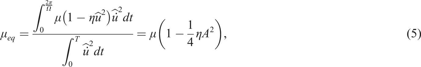
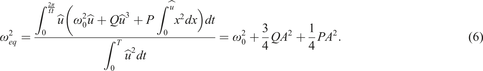
It is noted that the damping coefficient and the frequency formulations found in Equations (5) and (6) are completely different from the frequency formula obtained by He–Liu’s modification. ¹⁷ The integrations of El-Dib’s formula^11,13 are particularly related to the independent variable t. Moreover, the integration limits are impacted by the period T. Nevertheless, the integrations of He–Liu’s modification are related to the constant amplitude A. El-Dib’s formula ¹² can be used to derive consecutive approximations of solutions, but He–Liu’s formula cannot. In addition, He–Liu’s modification ¹⁷ is unable to determine the frequency when the nonlinear stiffens function involves velocity or a combination of the displacement and velocity. Furthermore, this paper’s equations (5) and (6) do not originate from He–Liu’s revision. ¹⁷ Refer to^13,26 for further information. Furthermore, as shown in Ref. 37, El-Dib’s formula can be utilized to relax the quadratic nonlinearity and the external periodic force, whereas He–Liu’s modification cannot.

The precise form of the analytical solution to equation (3) is as follows ³⁸

$u\left(t\right)=\left(A-\frac{q\left({\omega }_{eq}^2-{\omega }^2\right)}{\left({\left({\omega }_{eq}^2-{\omega }^2\right)}^2+4{\mu }_{eq}^2{\omega }^2\right)}\right)e^{-{\mu }_{eq}t}\hspace{0.17em}\mathit{cos}\hspace{0.17em}\Omega t+\frac{q\left(\left({\omega }_{eq}^2-{\omega }^2\right)\mathit{cos}\hspace{0.17em}\omega t+2{\mu }_{eq}\hspace{0.17em}\mathit{sin}\hspace{0.17em}\omega t\right)}{\left({\left({\omega }_{eq}^2-{\omega }^2\right)}^2+4{\mu }_{eq}^2{\omega }^2\right)}+\frac{{\mu }_{eq}}{\Omega }\left(A-\frac{q\left({\omega }_{eq}^2+{\omega }^2\right)}{\left({\left({\omega }_{eq}^2-{\omega }^2\right)}^2+4{\mu }_{eq}^2{\omega }^2\right)}\right)e^{-{\mu }_{eq}t}\hspace{0.17em}\mathit{sin}\hspace{0.17em}\Omega t,$

(7)

where the damping effect and nonlinear effects are covered by the frequency Ω, which is given by

${\Omega }^2={\omega }_{eq}^2-{\mu }_{eq}^2={\omega }_0^2+\frac{1}{4}\left(3Q+P\right)A^2-{\mu }^2{\left(1-\frac{1}{4}\eta A^2\right)}^2.$

(8)

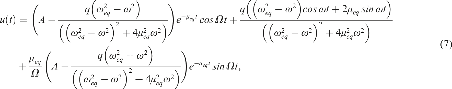
The numerical solution of equation (1) has been compared, as shown in Refs. 37,38, confirming the validity of the analytical solution (7).

It is observed that the simplest frequency level represented by equation (8) does not account for the contributions of the periodic force. To explore a more advanced level of frequency that includes the effects of the periodic force, it becomes necessary to modify the trial solution presented in equation (4). This modification is a crucial step towards deriving an advanced solution for the linearized equation, which is equation (3), as opposed to relying on the primary solution outlined in equation (7). The development of (equation (5)) this advanced solution is instrumental in enabling a comprehensive study of the stability behavior of the system and facilitates a detailed discussion of resonance responses. Such an approach is vital for a deeper understanding of the dynamics at play, particularly in examining how external periodic forces influence the system’s behavior and stability.

Construct an advanced approximate solution

To investigate stability in both the non-resonance and resonance cases, beyond the scope of the established primary solution (equation (7)), an advanced approach is employed. The benefits of the approach outlined here enable the trial solution to examine vibrational behavior in resonance response and provides new modeling tools. This method shows how crucial resonance characteristics are in determining a system’s behavior in the presence of outside excitations. This approach involves constructing a sophisticated approximate solution for equation (3). The development of this advanced solution is key to exploring the presence of resonance in the system. To initiate this process, the linearized form of equation (3) serves as the starting point. This methodological shift is pivotal for a comprehensive analysis, allowing for a nuanced understanding of the system’s dynamics, particularly concerning resonance phenomena. By delving into these advanced solutions, the study aims to uncover deeper insights into the oscillatory behavior of the system under various conditions, especially focusing on the critical points of resonance and stability.

Examining solution (7) reveals that division by zero does not occur, which means the denominator of the fraction never approaches zero. Consequently, the solution in equation (7) indicates the absence of a resonance scenario. This outcome is expected, as equation (3) represents a linear oscillation. In resonance analysis, the focus is typically on the presence of nonlinearity. ¹ Our approach requires an advanced analysis to discuss the behavior of the periodic force in resonance cases, even in the absence of nonlinearity. The trial solution (4) is inadequate for fully understanding the harmonic resonance scenario of equation (3). As a result, a comprehensive global frequency, denoted as Θ, needs to be considered. This frequency governs the entire system, including the effects of the periodic force. Therefore, an advanced trial solution is required, one that incorporates this unknown advanced frequency Θ and accounts for the efficiency of the periodic force

$U\left(t\right)=\left(A-\gamma \right)\mathit{cos}\hspace{0.17em}\Theta t+\gamma \hspace{0.17em}\mathit{cos}\hspace{0.17em}\omega t.$

(9)

In the proposed research, γ represents an unknown amplitude that is crucial for studying the existence of resonance response. The suggested solution (9) is designed to converge to the initial, constant amplitude A as it approaches zero. This advanced trial solution incorporates the frequency ω of the periodic force along with the unknown amplitude γ. Additionally, Θ signifies the new unknown system frequency. The structure of this new trial solution is crafted to replicate the primary solution (7). ¹² This arrangement is essential to facilitate the discussion on the occurrence of the resonance response.

The benefit of using the Galerkin method

Indeed, when dealing with trial solutions involving more unknowns, it becomes imperative to obtain two equations to determine these unknowns effectively. The Galerkin method serves as a powerful tool for achieving this goal, particularly in models involving nonlinearities and complex dynamics. The Galerkin method allows us to convert the original differential equation into a set of differential equations by projecting the residual (the difference between the original equation and the trial solution) onto a suitable set of basis functions. ³⁸ By choosing appropriate basis functions, we can ensure that the resulting equations capture the essential dynamics of the system while simplifying the problem.

In the context of trial solutions like equation (9), where two unknowns need to be determined, the Galerkin method enables us to obtain a system of equations by imposing orthogonality conditions on the residual concerning two different basis functions. These equations can then be solved to find the values of the unknowns, thereby providing a complete solution to the problem.

Overall, the Galerkin method offers a systematic and efficient approach to solving differential equations with trial solutions involving multiple unknowns. Its ability to generate a set of equations from the original problem makes it particularly well-suited for addressing complex nonlinear systems and obtaining accurate solutions in various scientific and engineering applications.

Implementing the Galerkin approach will be instrumental in achieving our objective. To construct the residual function $\mathit{R}\left(\mathbf{\Theta };\mathit{t}\right)=\mathbf{0}$ , solution (9) is applied to the non-homogeneous equation (3), which includes the explicit presence of the periodic force. This application results in a specific residual function that reflects the discrepancies between the exact solution and the approximate trial solution. The residual function is a key aspect of Galerkin’s approach, allowing for the optimization of the trial solution parameters to minimize the residual, thereby enhancing the accuracy of the approximate solution. ³⁹ The process of determining the optimal parameters typically involves solving a set of equations derived from the residual function, ensuring the best possible approximation of the system’s behavior under the influence of periodic forcing. This methodology is vital for comprehensively understanding and predicting the dynamics of the system, particularly in the context of resonance phenomenon

$R\left(\Theta ;t\right)=\left(A-\gamma \right)\left(\left({\Theta }^2-{\omega }_{eq}^2\right)\mathit{cos}\hspace{0.17em}\Theta t+2{\mu }_{eq}\Theta \hspace{0.17em}\mathit{sin}\hspace{0.17em}\Theta t\right)+\left(q+\gamma \left(-{\omega }_{eq}^2+{\omega }^2\right)\right)\mathit{cos}\hspace{0.17em}\omega t+2{\mu }_{eq}\gamma \omega \hspace{0.17em}\mathit{sin}\hspace{0.17em}\omega t.$

(10)

Given that Θ and γ are our two unknowns, the Galerkin integral should be found in the following forms

${\displaystyle {\int }_0^T}\left(A-\gamma \right)\left(\left({\Theta }^2-{\omega }_{eq}^2\right){\mathit{cos}}^2\hspace{0.17em}\Theta t+2{\mu }_{eq}\Theta \hspace{0.17em}{\mathit{sin}}^2\hspace{0.17em}\Theta t\right)dt=0;T=\frac{2\pi }{\Theta },$

(11)

In terms of $\gamma \hspace{0.17em}\mathit{cos}\hspace{0.17em}\omega t$ and $\gamma \hspace{0.17em}\mathit{sin}\hspace{0.17em}\omega t$ then using Galerkin integral again yields

${\displaystyle {\int }_0^T}{\left(\left(q+\gamma \left(-{\omega }_{eq}^2+{\omega }^2\right)\right){\mathit{cos}}^2\hspace{0.17em}\omega t+2{\mu }_{eq}\gamma \omega \hspace{0.17em}{\mathit{sin}}^2\hspace{0.17em}\omega t\right)|}_{\omega \to \sigma /T}dt=0;T=\frac{2\pi }{\Theta }.$

(12)

The parameter σ serves as a dimensionless representation of the applied frequency ω. Scaling by the period T is used to obtain this representation. The dimensionless form of σ/T provides a standardized way to express frequencies relative to the period of the oscillation, enabling easier comparison and analysis across different systems. Overall, this representation provides clarity on the relationship between ω and σ and their significance in the analysis of periodic systems.

Obtaining the aforementioned integrals yields the subsequent equations

$-\pi \left(A-\gamma \right)\left({\Theta }^2+2{\mu }_{eq}\Theta -{\omega }_{eq}^2\right)=0,$

(13)

$\frac{1}{8\pi \sigma \Theta }\left(-2\sigma \left(4\pi \gamma {\mu }_{eq}\sigma \Theta +\gamma {\sigma }^2{\Theta }^2+4{\pi }^2\left(q-\gamma {\omega }_{eq}^2\right)\right)+\left(4\pi \gamma {\mu }_{eq}\sigma \Theta -\gamma {\sigma }^2{\Theta }^2-4{\pi }^2\left(q-\gamma {\omega }_{eq}^2\right)\right)\mathit{sin}\hspace{0.17em}2\sigma \right)=0.$

(14)

To express equation (13) with the distinction between the unknown amplitude γ and the oscillation amplitude A, we can make the following appropriate

${\Theta }^2+2{\mu }_{eq}\Theta -{\omega }_{eq}^2=0.$

(15)

After this, we can rearrange the terms of equation (14) to obtain a quadratic form in Θ. However, the specific form of the resulting quadratic equation will depend on the expression for the unknown γ and σ

$\gamma {\sigma }^2\left(2\sigma +\mathit{sin}\hspace{0.17em}2\sigma \right){\Theta }^2+4\pi \gamma {\mu }_{eq}\sigma \left(2\sigma -\hspace{0.17em}\mathit{sin}\hspace{0.17em}2\sigma \right)\Theta +4{\pi }^2\left(q-\gamma {\omega }_{eq}^2\right)\left(2\sigma +\mathit{sin}\hspace{0.17em}2\sigma \right)=0.$

(16)

The frequency Θ, which is the first unknown, is obtained by solving equation (15)

$\Theta =-{\mu }_{eq}+\sqrt{{\mu }_{eq}^2+{\omega }_{eq}^2}.$

(17)

When Θ is removed from equations (15) and (16) the second unknown γ is expressed as

$k_2{\gamma }^2+k_1\gamma +k_0=0.$

(18)

As observed equation (18) is a quadratic equation in the amplitude γ with two roots, γ₁ and γ₂. These origins are provided by

${\gamma }_{1,2}=\frac{1}{2k_2}\left(-k_1\pm \sqrt{k_1^2-4k_0{k}_2}\right).$

(19)

where

$k_2={\omega }_{eq}^2\left(\begin{array}{l}4{\sigma }^2{\left(-2\pi +\sigma \right)}^2\left(\left(4{\pi }^2+{\sigma }^2\right){\omega }_{eq}^2+4\pi \sigma \left(2{\mu }_{eq}^2+{\omega }_{eq}^2\right)\right)+4\sigma {\left(-4{\pi }^2+{\sigma }^2\right)}^2{\omega }_{eq}^2\hspace{0.17em}\mathit{sin}\hspace{0.17em}2\sigma \\ +{\left(2\pi +\sigma \right)}^2\left(\left(4{\pi }^2+{\sigma }^2\right){\omega }_{eq}^2-4\pi \sigma \left(2{\mu }_{eq}^2+{\omega }_{eq}^2\right)\right){\mathit{sin}}^2\hspace{0.17em}2\sigma \end{array}\right),$

(20)

$k_1=-8{\pi }^{2}q\left(2\sigma +\mathit{sin}\hspace{0.17em}2\sigma \right)\left(\begin{array}{l}2\sigma \left(4\pi {\mu }_{eq}^2\sigma +4{\pi }^2{\omega }_{eq}^2-{\sigma }^2\left(2{\mu }_{eq}^2+{\omega }_{eq}^2\right)\right)\\ +\left(2\pi +\sigma \right)\left(-2{\mu }_{eq}^2\sigma +\left(2\pi -\sigma \right){\omega }_{eq}^2\right)\mathit{sin}\hspace{0.17em}2\sigma \end{array}\right),$

(21)

$k_0=16{\pi }^4{q}^2{\left(2\sigma +\mathit{sin}\hspace{0.17em}2\sigma \right)}^2.$

(22)

The non-resonance scenario is defined as one in which the denominator of the amplitude γ is incapable of tending to zero. A resonant case or a singularity is produced by the zero denominator. This concludes the non-resonance case solution, which has the form

$u\left(t\right)=e^{-{\mu }_{eq}t}\left(A-{\gamma }_i\right)\left(\mathit{cos}\hspace{0.17em}\Theta t+\frac{{\mu }_{eq}}{\Theta }\mathit{sin}\hspace{0.17em}\Theta t\right)+{\gamma }_i\hspace{0.17em}\mathit{cos}\hspace{0.17em}\omega t;i=1,2,$

(23)

It should be noticed that the standard exact solution found at the primary solution (7) is replicated by the above-advanced solution.

Stability behavior for the non-resonance case

Requiring Θ to be real to meet the stability criteria, the following stability conditions that satisfy the non-resonance case can be obtained from the discriminant of both equations (15) and (16):

${\omega }_{eq}^2+{\mu }_{eq}^2>0,$

(24)

$\left({\left(2\sigma -\hspace{0.17em}\mathit{sin}\hspace{0.17em}2\sigma \right)}^2{\mu }_{eq}^2+\pi {\left(2\sigma +\mathit{sin}\hspace{0.17em}2\sigma \right)}^2{\omega }_{eq}^2\right)\gamma -\pi q{\left(2\sigma +\mathit{sin}\hspace{0.17em}2\sigma \right)}^2>0.$

(25)

The requirement of stability equation (25) can be interpreted as

$\gamma >{\gamma }^{*}=\frac{\pi q{\left(2\sigma +\mathit{sin}\hspace{0.17em}2\sigma \right)}^2}{{\left(2\sigma -\hspace{0.17em}\mathit{sin}\hspace{0.17em}2\sigma \right)}^2{\mu }_{eq}^2+\pi {\left(2\sigma +\mathit{sin}\hspace{0.17em}2\sigma \right)}^2{\omega }_{eq}^2}.$

(26)

Due to (19), it is possible to seek the stability condition (26) as

$k_2\left(k_2{{\gamma }^{*}}^2+k_1{\gamma }^{*}+k_0\right)<0.$

(27)

The notations (20)–(22) guarantee that the square forced amplitude parameter q can be immediately canceled from the previous condition, hence removing the parameter’s dependence on the remaining condition.

Discussion of the stability behavior due to the resonance case

To study the stability behavior at the resonance case we may solve equation (16) for the amplitude γ yields

$\gamma =\frac{4q{\pi }^2\left(2\sigma +\mathit{sin}\hspace{0.17em}2\sigma \right)}{\left(4{\pi }^2{\omega }_{eq}^2-{\sigma }^2{\Theta }^2\right)\left(2\sigma +\mathit{sin}\hspace{0.17em}2\sigma \right)-4\pi {\mu }_{eq}\sigma \left(2\sigma -\hspace{0.17em}\mathit{sin}\hspace{0.17em}2\sigma \right)\Theta }.$

(28)

In the resonance scenario, equation (28) has a denominator that approaches zero. One can introduce the so-called detuning parameter δ ≠0, which is defined as follows, to prevent the division by zero:

$\left(4{\pi }^2{\omega }_{eq}^2-{\sigma }^2{\Theta }^2\right)\left(2\sigma +\mathit{sin}\hspace{0.17em}2\sigma \right)-4\pi {\mu }_{eq}\sigma \left(2\sigma -\hspace{0.17em}\mathit{sin}\hspace{0.17em}2\sigma \right)\Theta =\delta .$

(29)

The amplitude γ can be used in terms of the parameter δ by using equation (29) into equation (28) as

$\gamma =\frac{4q{\pi }^2\left(2\sigma +\mathit{sin}\hspace{0.17em}2\sigma \right)}{\delta }.$

(30)

To rewrite the amplitude equation in terms of the parameter δ, insert equation (30) into equation (18) as follows:

${\delta }^2+h_1\delta +h_0=0,$

(31)

with the two roots

${\delta }_{1,2}=-\frac{h_1}{2}\pm \frac{1}{2}\sqrt{h_1^2-4h_0},$

(32)

where

$h_1=4q{\pi }^2\left(2\sigma +\mathit{sin}\hspace{0.17em}2\sigma \right)\frac{k_1}{k_0},$

(33)

$h_0=16q^2{\pi }^4{\left(2\sigma +\mathit{sin}\hspace{0.17em}2\sigma \right)}^2\frac{k_2}{k_0}.$

(34)

Applying the discriminant property of the quadratic equation (29) to get the condition on Θ to be real imposes the following stability condition in terms of the detuning parameter δ

$\delta <{\delta }^{*}=\frac{4{\pi }^2\left({\mu }_{eq}^2{\left(2\sigma -\hspace{0.17em}\mathit{sin}\hspace{0.17em}2\sigma \right)}^2+{\omega }_{eq}^2{\left(2\sigma +\mathit{sin}\hspace{0.17em}2\sigma \right)}^2\right)}{\left(2\sigma +\mathit{sin}\hspace{0.17em}2\sigma \right)}.$

(35)

Eliminate δ from the stability condition (35) with the help of equation (32) leads to

${{\delta }^{*}}^2+{\delta }^{*}{h}_1+h_0>0.$

(36)

It is noted that the amplitude q does not affect the stability condition (36). The amplitude γ at the resonance case can be symbolized by γ _r which can be performed by employing equation (32) into equation (30) to have

${\gamma }_r=\frac{8q{\pi }^2\left(2\sigma +\mathit{sin}\hspace{0.17em}2\sigma \right)}{-h_1\pm \sqrt{h_1^2-4h_0},}.$

(37)

The advanced approximated periodic solution at the resonance case is expressed in the form

$u\left(t\right)=e^{-{\mu }_{eq}t}\left(A-{\gamma }_r\right)\left(\mathit{cos}\hspace{0.17em}\Theta t+\frac{{\mu }_{eq}}{\Theta }\mathit{sin}\hspace{0.17em}\Theta t\right)+{\gamma }_r\hspace{0.17em}\mathit{cos}\hspace{0.17em}\omega t.$

(38)

Discussion and numerical illustration

Correct, nonlinear equations typically lack exact analytical solutions due to their inherent complexity. However, in some cases, nonlinear differential equations can be approximated by equivalent linear equations, which may have exact solutions under certain conditions.

In the context of the discussion, a solution obtained for a non-homogeneous linear equation (such as equation (3)) that does not contain variable coefficients. This solution serves as an approximation for the original nonlinear equation (equation. (1)). While it may not perfectly capture all aspects of the nonlinear system’s behavior, it provides a useful approximation that can yield valuable insights into the system’s dynamics. It’s important to note that this solution for the linear equation is obtained through mathematical techniques such as the non-perturbative method, which transforms the original nonlinear system into an equivalent linear form. While this solution may not precisely represent the behavior of the nonlinear system in all cases, it serves as a valuable tool for analysis and understanding, particularly when dealing with complex nonlinear dynamics.

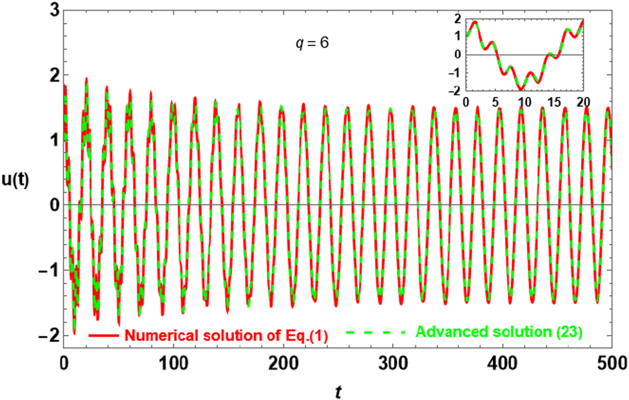
To examine the accuracy of an approximate solution (23), we have shown many graphs to numerically compare it with the numerical solution of equation (1). Figures (1) through (5) show this corresponding. Different values of the amplitude q were used in the computations for slightly tiny values of the parameter σ (σ = 0.1). For the stimulated force in Figure (1), q = 0.1 is the selected amplitude. The comparison shows that the exact solution generated from the conventional trial solution (4) and the analytical solution (23), acquired using the advanced trial method (9), agree quite well. This graph shows that the damping effect outweighs the external force’s periodic effects. It is observed that the vibration’s amplitude steadily drops over an extended length of time, showing that the force applied to the system had no effect.

Figure 1.

Comparison of the advanced solution (23) with the numerical solution of equation (1) in the case of small q and large σ for a system having $P=0.1,{\omega }_0=2,Q=0.1,\eta =0.1,\mu =0.01,\sigma =0.1,A=1.$

Figure 2.

(a): Comparison of the advanced solution (23) with the numerical solution of equation (1) for the same system given in Figure 1 with increased q to become q = 1. (b): Comparison of the advanced solution (23) with the numerical solution of equation (1) for the same system given in Figure 1 with increased q to become q = 1.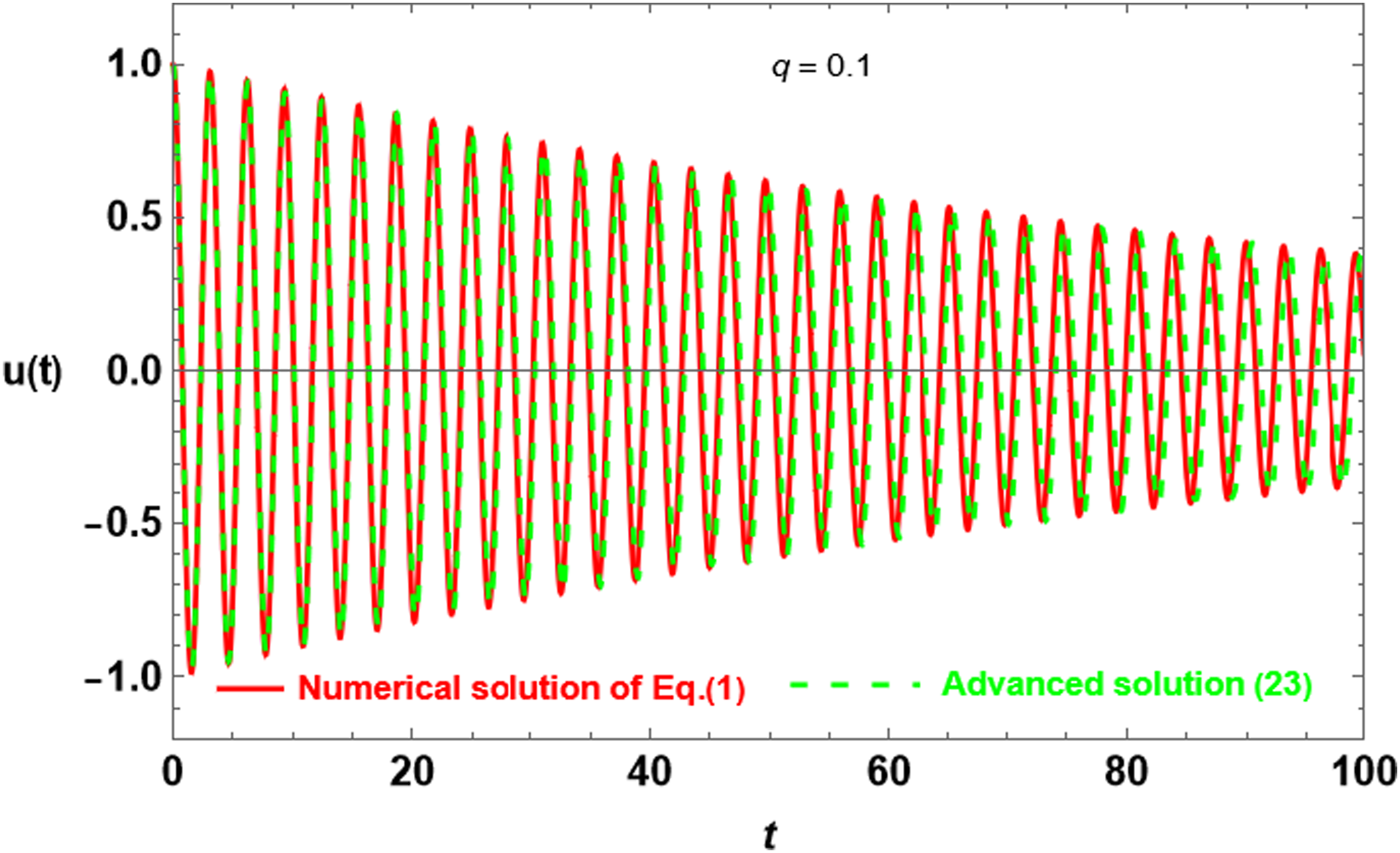

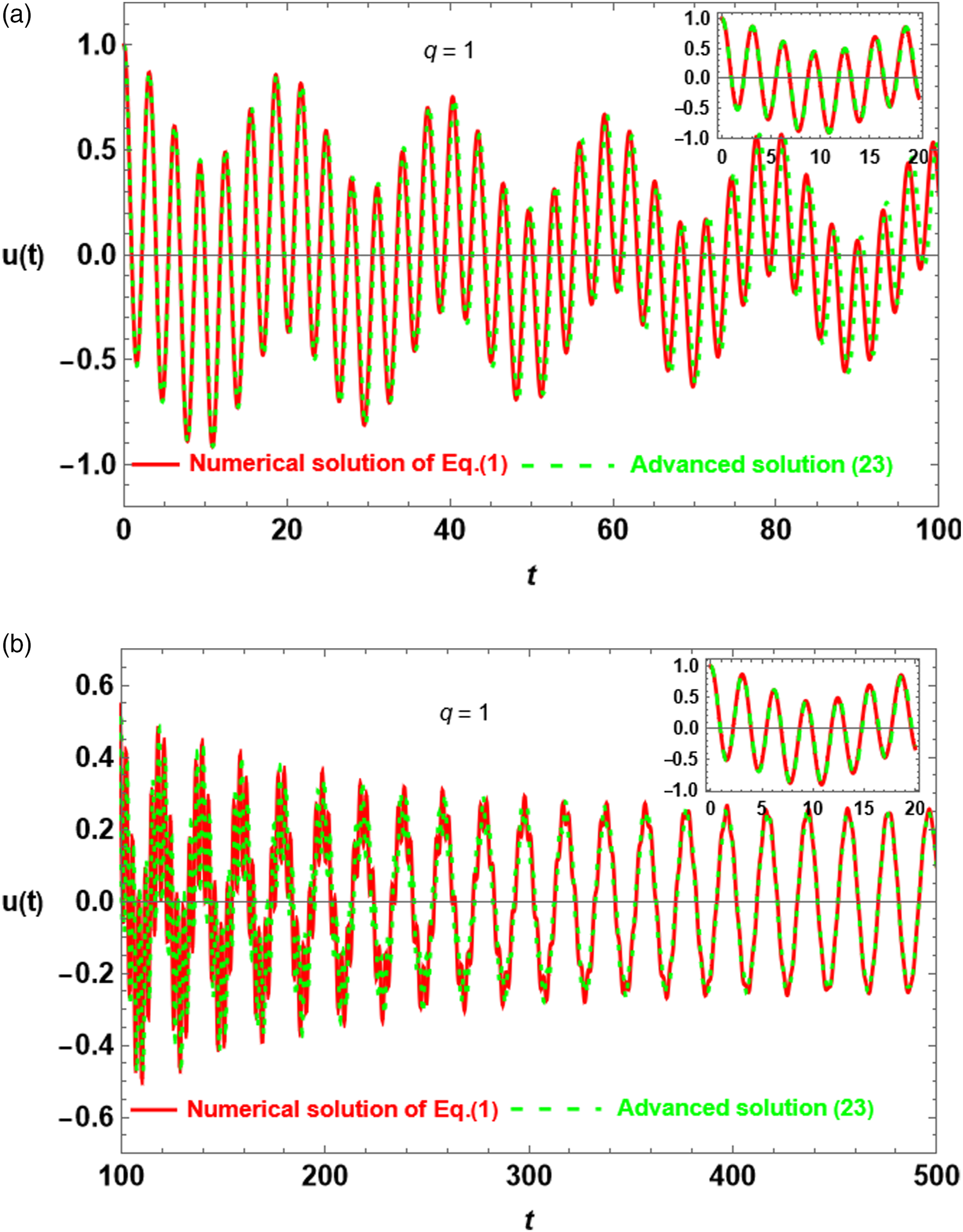
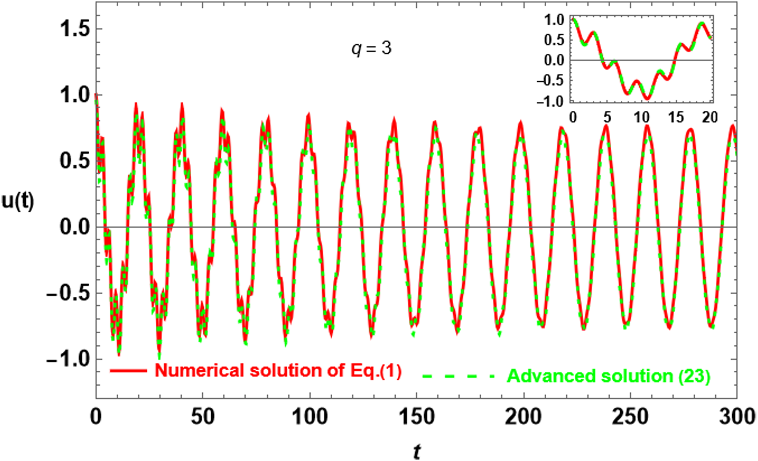
Figure 3.

Comparison of the advanced solution (23) with the numerical solution of equation (1) in the case of an increase q to the value 3, for the same system given in Figure 1.

Figure 4.

Comparison of the advanced solution (23) with the numerical solution of equation (1) in the case of q = 4 for the same system given in Figure 1.

Figure 5.

Comparison of the advanced solution (23) with the numerical solution of equation (1) in the case of q = 6 for the same system given in Figure 1.

Setting the force amplitude value to q = 1, as shown in Figure 2(a), causes the vibration to repeat in a decreasing pattern over a predetermined amount of time. An ascending cycle starts following each damping phase, and this oscillatory behavior continues with a constant decrease in vibration amplitude. As shown by Figure 2(a), this phenomenon lasts for a long amount of time. The time frame in Figure 2(b) shows that the damping phase terminates after a long time. It goes from t = 100 to t = 500. The periodic effect of the outside power then takes over and doesn’t stop. Interestingly, during these stages, there is consistent agreement between the analytical solution (23) and the exact solution (7). The periodic resonance caused by the applied force begins to occur sooner when the amplitude of the periodic force is increased to q = 3, as shown in Figure (3), whereupon the damping effect is quickly reduced.

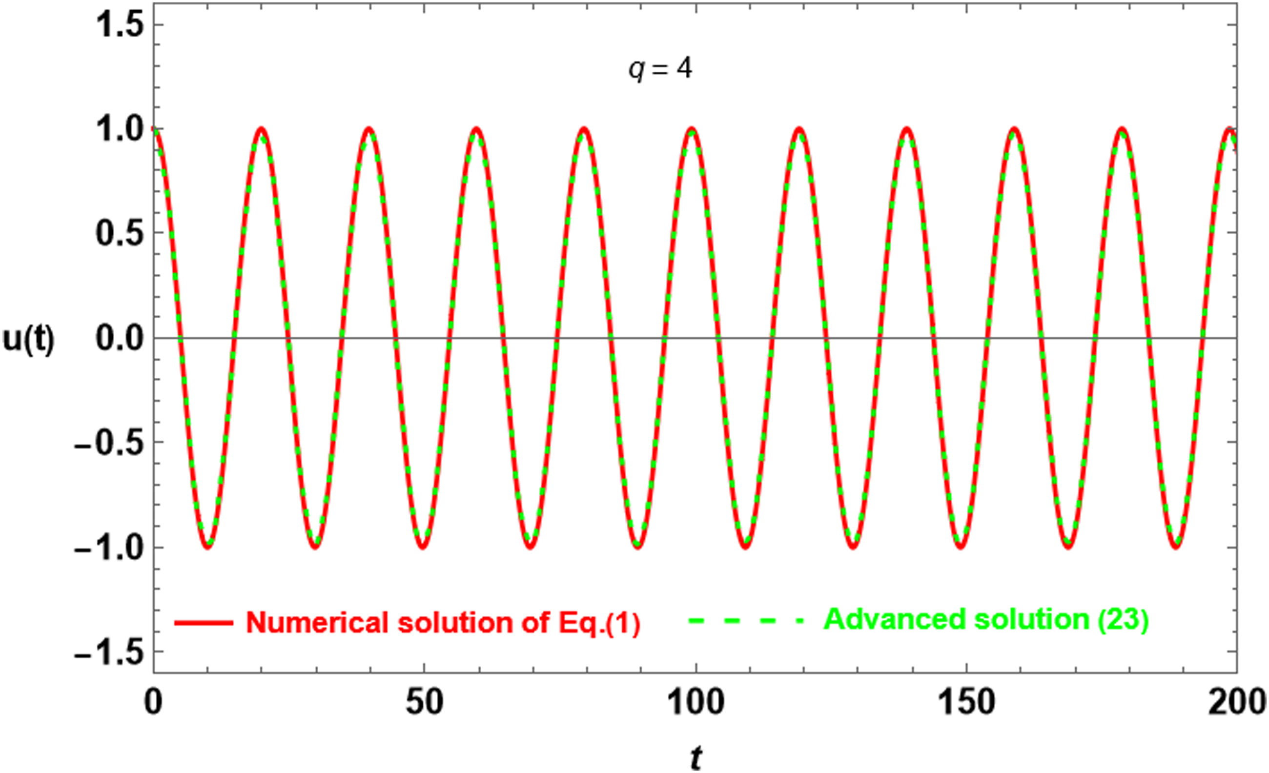
The damping effect is reduced and the cyclic nature of the force primarily affects the vibrational behavior when the amplitude of the periodic force is increased to q = 4, as seen in Figure (4). This outcome is especially noteworthy since it shows how periodic force can counteract unfavorable consequences in the system. The damping effect gradually reappears in Figure (5) as the force amplitude is further elevated to q = 6, and the periodic external force’s influence correspondingly decreases. This finding implies that there is a threshold for attaining continuous periodic vibration and that there is an ideal amplitude for the applied force beyond which the system’s net vibration returns to a damped condition.

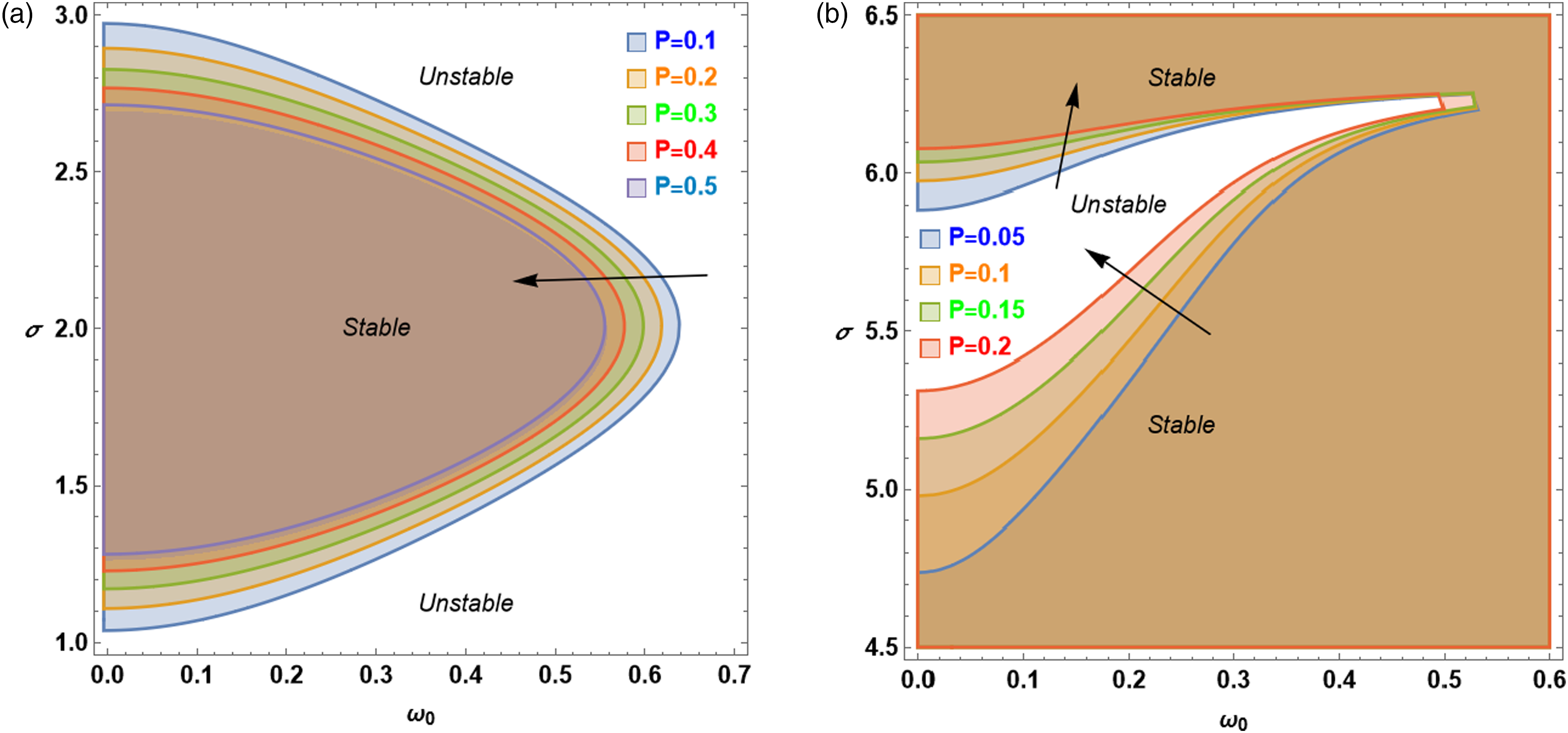
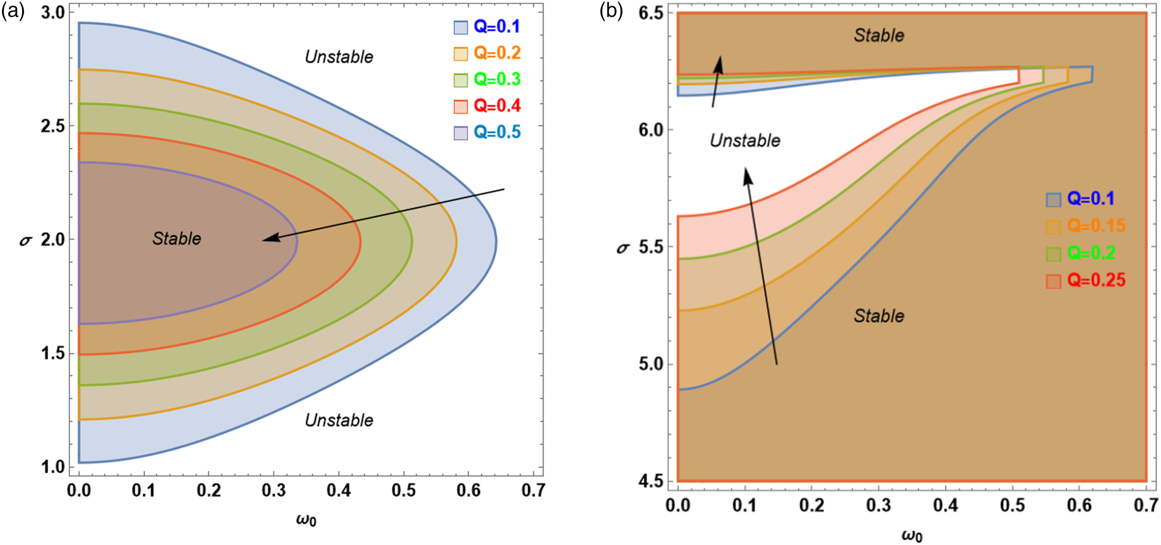
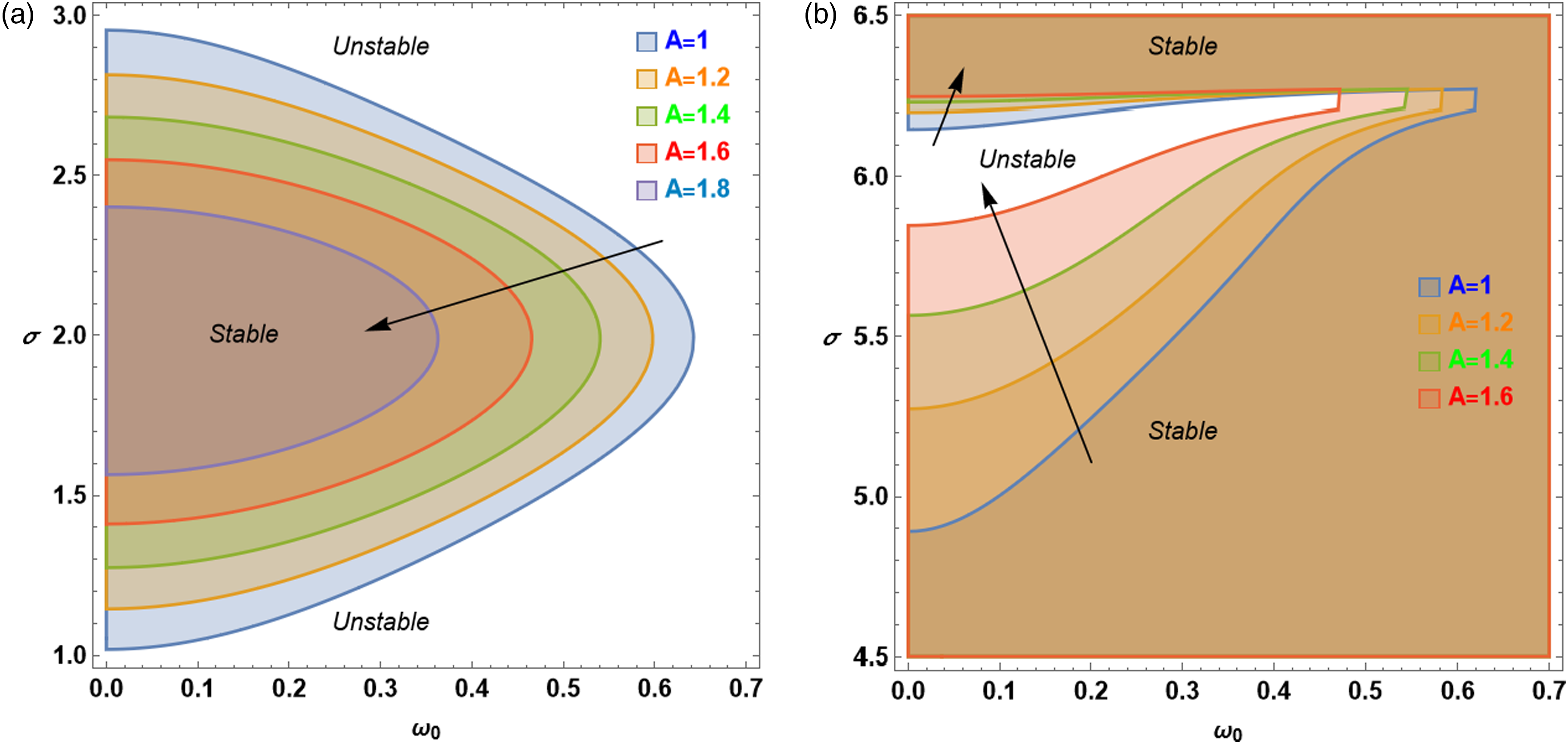
Figures (6–9(a)) graphically exhibit the stability condition (27) in the non-resonance situation, and Figures (6–9(b)) graphically represent the stability condition (36), relevant to the resonance scenario. The purpose of these figures is to investigate how the basic system characteristics affect stability behavior in both the non-resonant and resonant states. The plane of σ versus the natural frequency ω₀ is used to do the stability analysis. A visual grasp of how different conditions affect the stability of the system is provided by the graphical displays of stability conditions (27) and (36) that divide the plane (σ- ω₀) into stable and unstable regions.

Figure 6.

(a): Effect of the variation of the damping coefficient μ on the stability behavior for the non-resonance case as given by condition (27) for a system having P = Q = η = 0.1 and A = 1. (b): Effect of the variation of the damping coefficient μ on the stability behavior for the resonance case as given by the condition (36) for the same given in Figure 6(a).

Figure 7.

(a): Effect of the variation of the nonlinear quadratic coefficient P on the stability behavior for the non-resonance case as given by condition (27) for the same system given in Figure 6(a) except that μ = 0.1. (b): Effect of the variation of the nonlinear quadratic coefficient P on the stability behavior for the non-resonance case as given by condition (36) for the same system given in Figure 6(a) except that μ = 0.1.

Figure 8.

(a): Effect of the variation of the nonlinear cubic coefficient Q on the stability behavior for the non-resonance case as given by the condition (27) for the same system given in Figure 6(a). (b): Effect of the variation of the nonlinear cubic coefficient Q on the stability behavior for the non-resonance case as given by the condition (36) for the same system given in Figure 8(a) except that μ = 0.2.

Figure 9.

(a): Effect of the variation of amplitude A on the stability behavior for the non-resonance case as given by the condition (27) for the same system given in Figure 6(a). (b): Effect of the variation of amplitude A on the stability behavior for the non-resonance case as given by the condition (36) for the same system given in Figure 8(b).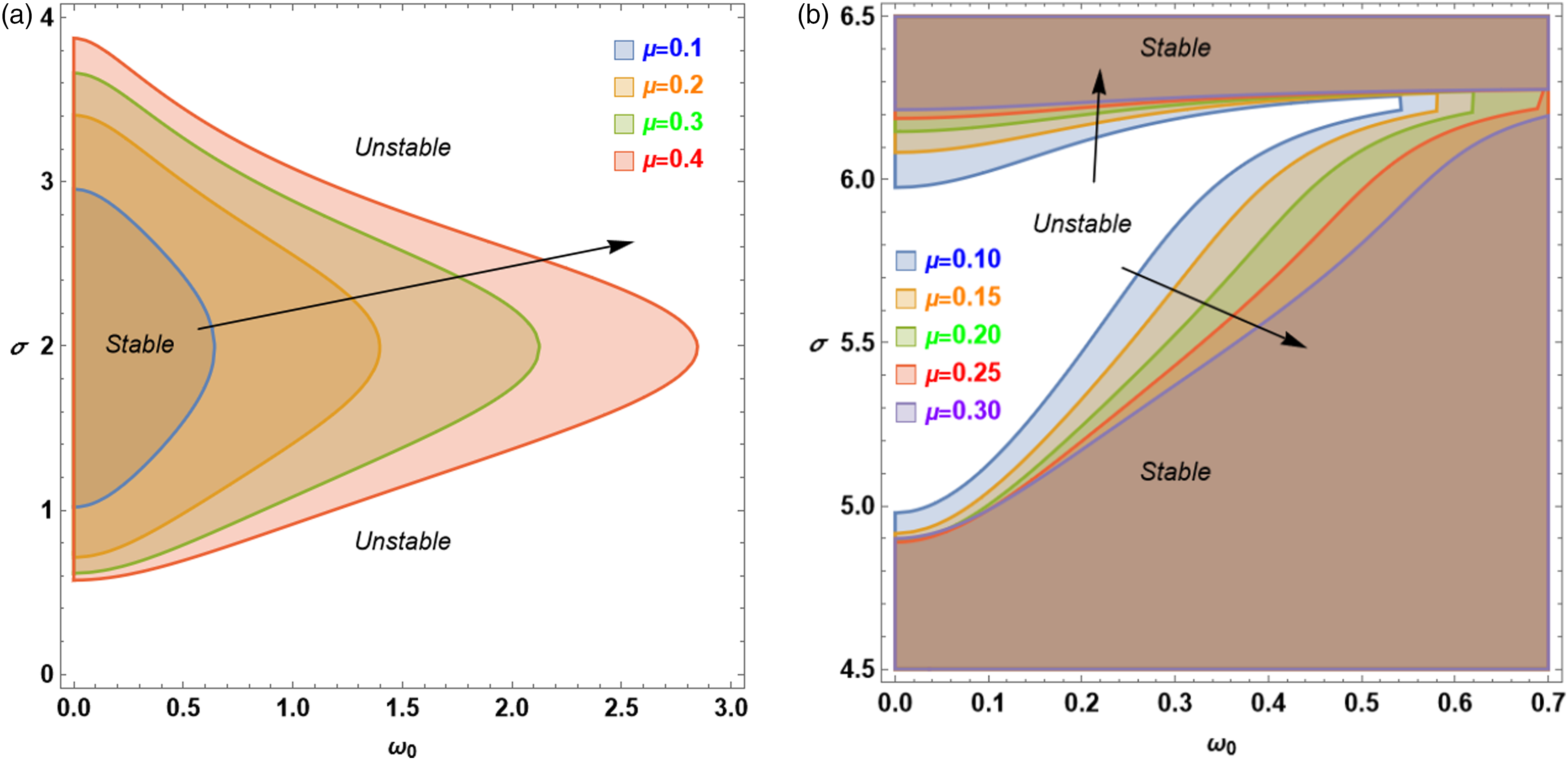

The examination of the impact of the linear damping parameter μ on the stability picture in the non-resonance case is shown in Figure 6(a) and in the resonance case which is displayed in Figure 6(b). Figure 6(a) shows that the increase in μ works to expand the stability zone so that it includes a greater period of stability relative to the parameter σ, with expansion in the direction of increasing ω₀. This observation means that the increase in μ has a stabilizing influence in the non-resonance case. This is the usual role for the linear damping influence.

Figures 6(a) and 6(b) show how stability is affected by the linear damping parameter μ in the non-resonance and resonance instances, respectively. As can be seen in Figure 6(a), a rise in μ broadens the stability zone, extending towards higher ω₀ values and covering a wider range of stability concerning the parameter σ. This implies that a rise in μ stabilizes the non-resonance situation, consistent with the traditional interpretation of the role of linear damping. On the other hand, Figure 6(b) investigates the resonance situation and offers information about how the linear damping parameter affects the dynamic variations in stability behavior.

In Figure 6(b), where stability condition (36) is considered, the unstable resonance region appears intermingled within the stability region. The resonance region’s width is largest at the smallest value of ω₀ and decreases as ω₀ increases, eventually disappearing at relatively large ω₀ values. Upon further analysis, it was observed that increasing μ leads to an expansion of the resonance zone at the expense of the stability zone. This behavior indicates that μ exerts an unstable effect in the resonance region, contrasting with its stabilizing influence in the non-resonance case, as illustrated in Figure 6(a). This highlights the nuanced role of the damping parameter in different dynamic regimes of the system.

The study on the impact of nonlinear parameters, specifically the Helmholtz coefficient P, the Duffing coefficient Q, and the oscillation amplitude A, on stability behavior is illustrated in Figures (7–9), respectively. As denoted previously, figures marked with the letter “a” pertain to the non-resonance case, while those marked with “b” refer to the resonance case. Typically, it’s observed that the nonlinear coefficients and the amplitude A exhibit an unstable effect in the non-resonance case. Conversely, in the resonance case, their role reverses, acting as a stabilizing influence on the system’s dynamics. This reversal highlights the significant and varied impact that nonlinear parameters have on system stability across different dynamic scenarios.

Conclusion

By using the analogous linearization approach on the nonlinear oscillator, the forced Van der Pol-Duffing-Helmholtz oscillator in the present study has been transformed into a forced damping linear oscillator. The usual exact solution derived by the normal form technique cannot be used to study the stability behavior in the resonance scenario due to the influence of the imposed frequency. The frequency that is achieved by applying the normal form approach is not dependent on the frequency of the applied force. Due to this restriction, a different standard-like solution was created, allowing for the examination of stability behavior as well as a discussion of resonance. By applying an advanced trial solution to the given forced equivalent damping linearized equation, a residual equation is generated. The suggested trial solution’s unknowns are then located and investigated using the Galerkin approach in order to investigate the resonance phenomena. A numerical comparison is made between a visually depicted analytical solution and one produced through the use of the Galerkin approach. It is noticed that the effective amplitude of the periodic force at a given amplitude cancels out the damping effect. When comparing the resonance situation with the non-resonance condition, numerical computations show that all physical parameters reverse their mechanism.