This work studies the nonlinear movement of a two degrees-of-freedom (DOF) spring pendulum that is dampened and affected by a harmonic force externally. It is presumed that the spring’s pivot point travels along an elliptic route. Lagrange’s equations are utilized to generate the regulating system of motion. The multiple-scales approach (MSA) is used to gain the system’s analytic solutions up to the third-order approximation. Therefore, all resonance cases that have emerged are categorized, wherein two of them are scrutinized at once. As a result of the removal of secular terms, the solvability constraints are attained and then the steady-state solutions are investigated. The examined motion’s temporal evolution, the resonance response curves, and the solutions at the steady-state are all depicted graphically. In compliance with the Routh–Hurwitz criteria (RHC), all possible fixed points (FPs) for the steady and unsteady cases are found and displayed. The stability zones are examined and analyzed to estimate the effect of various factors on the system’s behavior. This model has gained prominence recently due to its industrial uses in seismic isolation systems for buildings and structures. However, in seismic engineering, a 2DOF vibrating pendulum system can be used as part of a seismic isolation system designed to protect buildings and infrastructure from earthquake-induced vibrations. The pendulum mechanism helps to absorb and dissipate seismic energy, reducing the amount of force transmitted to the structure. During an earthquake, the ground motion acts as an external harmonic force on the building. The distribution of mass and the structural layout can cause rotational moments that act on the building. The pendulum system can be tuned to counteract these moments, helping to stabilize the structure. The pendulum system allows for both horizontal and vertical displacement, providing two degrees of freedom. This capability is essential for accommodating the complex, multi-directional nature of seismic waves.
Recently, many studies have appeared that deal with the nonlinear motion of vibratory systems in applied mechanics and study the effects of vibrations on structures, machines, vehicles, etc. The spring pendulum’s dampened motion,1–6 with linear or nonlinear stiffness, has contributed to addressing some of these problems. The case of internal resonance for the motion of a subjected elastic pendulum to an excitation force along its arm is studied in Reference 1, while the chaotic responses for its motion are examined in References 2 and 3. The positive impact of higher-order extensions on these responses is explored in Reference 4. It is found that the obtained solutions up to the second order outscored on the first approximations when looking at maximum Lyapunov exponents and bifurcation plots. In Reference 5, the procedure of the phase plane and the frequency response equation are used to examine the stability of this system. A modification of this study is examined in Reference 6 when the pendulum’s pivot point has a vertical oscillation.
The approximate solution of a 2DOF auto-parametric system is obtained in References 7 and 8 using the harmonic balancing method (HBM),9 where the chaotic reactions are numerically investigated for this system. Additionally, the investigation looks into the stable and unstable zones. The same methodology utilized was utilized in Reference 10 to investigate how a damped spring system responds to vibration under the impact of a harmonic excitation force. Examining the stability assessments of the obtained results confirms that the numerical outcomes are in high consistency with the approximate one. In Reference 11, the HBM is used to look at the solutions of the equations of motion (EOM) for a severely nonlinear oscillator coupled to a spring’s pendulum. Furthermore, the chaotic behavior of the spring is investigated as well as reducing the vibration near the parametric resonance. The method of averaging9 is utilized in Reference 12 to gain the approximate solution of an oscillating auto-parametric absorber. The limitations of stability and the analysis of bifurcation for the averaging system of EOM are investigated. In Reference 13, the influence of a vibrating auto-parametric absorber is examined. Reference 14 investigates the simple pendulum’s motion connected to a tuned absorber that is excited harmonically. The asymptotic solutions are acquired using MSA9 and represented graphically to show the impact of used parameters on the motion.
It should be highlighted that many academics have become interested in the damped motion of linear or nonlinear elastic pendulums in various pathways.15–25 In this regard, the planar motion of a harmonic oscillator close to resonance when the pivot point is assumed to move on trajectories of an ellipse and on a closed Lissajous curve is examined in References 26 and 15, respectively. A few limited circumstances for specified motions are provided. In Reference 16, the authors studied the stability analyses of a 3DOF dynamical system of a solid body attached to a damped linear spring with a fixed suspension point. The extensions of this problem are explored in References 17 and 18 with respect to the stiffness of linear and nonlinear springs. The pivot point of the pendulum was constrained to be on an ellipse. In References 19 and 20, a hard body pendulum is further described. Utilizing the MSA,9 the approximations are obtained, and the necessary modulation’s equations are achieved considering the constraints' solvability. The motion of various vibrating systems with the impact of harmonic external torques and forces is explored References 21–25 as well as the nonlinear analysis' stability for these systems.
The dynamical motion of a spring pendulum with weak nonlinearity is discussed in Reference 27, where its suspension point travels in a circular trajectory. The impact of a damper on the spring’s motion is examined in Reference 28 as a general case. The numerical study of this system for periodic, quasi-periodic, and chaotic motion is presented in Reference 29. Whereas in Reference 30 the authors examined the movements of a mass hanging with one end of a nonlinearly damped elastic pendulum under the effect of the spring’s transverse and radial forces, while the other end is considered to be fixed. The improvement of this work was found in Reference 31, where two methods with three time scales are used to decrease the error to a minimum. The EOM’s approximate solutions are obtained using MSA. To fulfill the solvability criteria, the secular term’s elimination condition is preserved. Most of the categories' resonances are studied. The stability criteria of the exact solution of a simple pendulum are explored in Reference 32, in which its fulcrum oscillates both horizontally and vertically. For a few distinct values of the pendulum’s parameters, a comparison of the obtained numerical and analytical solutions (AS) is presented. The periodic motions of a periodically forced nonlinear elastic pendulum are explored in Reference 33 using the semi-analytical approach, as well as the motion’s bifurcation and stability analyses. In Reference 34, RHC are used to explore the stability and instability zones, which are subsequently studied in terms of steady-state solutions. In Reference 35, the authors obtained analytical solutions of an oscillating 2DOF dynamical system using MSA. All possible FPs are determined in view of the examined resonance cases, while the stability of the triple pendulum is investigated using the nonlinear stability analysis approach in Reference 36. The integrated approach investigates the fractal modification of a nonlinear oscillator relevant to nanotechnology, as explored in prior studies.37–39 An improved harmonic balance method is used to solve the Duffing-harmonic equation.40 The variational approach is applied to solve different models.41–44 Some nonlinear oscillators are investigating by using the homotopy perturbation method.45,46
This article examines the nonlinear behavior of a 2DOF damped spring pendulum when external harmonic forces are applied. The spring’s pivot point is assumed to follow an elliptic path. Lagrangian equations are used to construct the EOM in accordance with the generalized coordinates of the system. Up to the third-order approximation, the desired solutions to these equations are acquired by using the MSA. According to the used perturbation approach, the used parameters may be written in terms of a small parameter. As a result, all discovered cases of resonance are grouped, with two of them examined concurrently. Once the elimination of secular terms, the solvability restrictions are fulfilled, and the solutions at the scenario of steady-state are then analyzed. The steady-state solutions, the resonance response curves, and the time evolution of the investigated motion are all pictorially displayed. All FPs are identified at this case and displayed in accordance with the RHC. To assess the good effects of different parameters on the motion’s behavior, the stability zones are examined and analyzed. Due to its industrial applications, the examined model is now widely used in seismic isolation systems to safeguard buildings and structures during earthquakes. The 2DOF vibrating pendulum system has become a key component in seismic isolation systems, protecting buildings and infrastructure from earthquake-induced vibrations.
Dynamical modeling
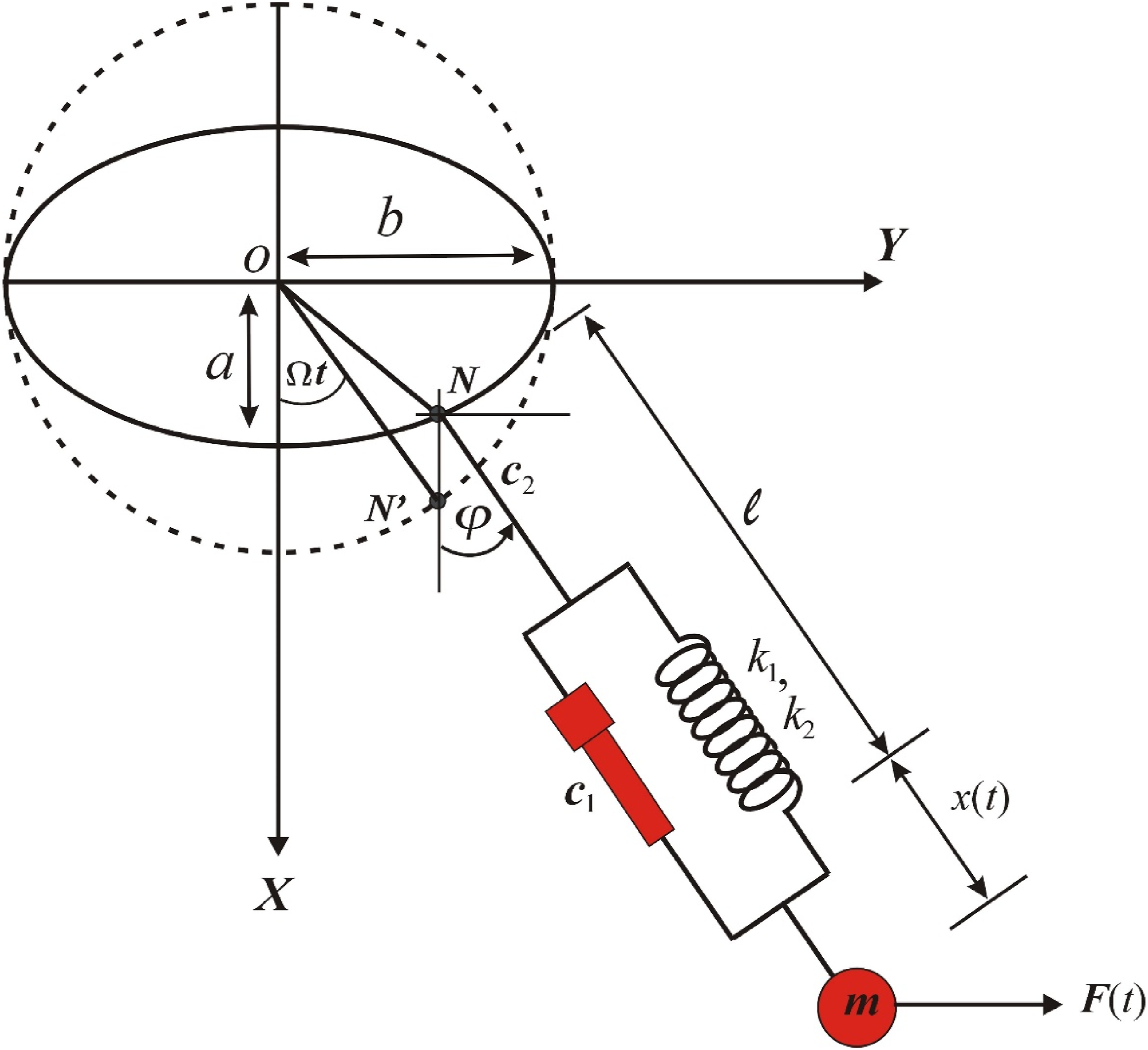
In this section, a vibrating pendulum system of a mass coupled to a damped massless spring with a natural length and stiffness and , which are the linear and nonlinear spring stiffness, respectively. Stiffness is typically measured in Newton’s per meter , but stiffness is typically measured in Newton’s per cubic meter (see Figure 1). The end is restricted to moving with a regular angular velocity on an elliptic path with radii and . The projections of on the axes and are and , respectively. On the dotted circle tangent to the ellipse of radius , it is noted that the point corresponds to the projection of the point on the dotted circle. The planar motion of the system is taken into account as the result of harmonic forces , in which and are, respectively, the frequencies and amplitudes of . Considering that is the dynamic spring’s extension, and are the coefficients of damping in both linear and seesaw vibrations.
The dynamical model.
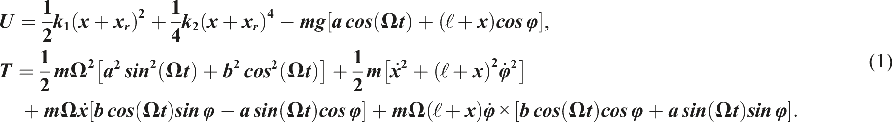
With the help of the previous description, the energies of potential and kinetic are expressed, respectively, in the form below
here in which is the static spring’s protraction, is the rotatory angle, and indicates the gravity’s acceleration.
The Lagrangian of the given model may be easily achieved. Consequently, the following Lagrangian equations can be used to obtain the EOM29
where and represent, respectively, the system’s generalized velocities and coordinates, while are the generalized forces that can be represented in the following forms
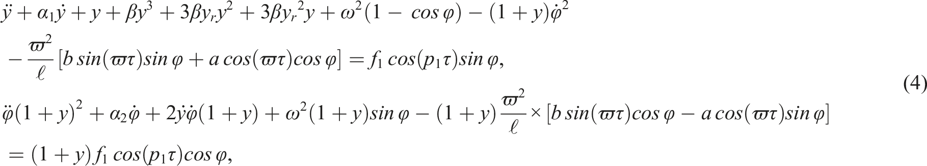
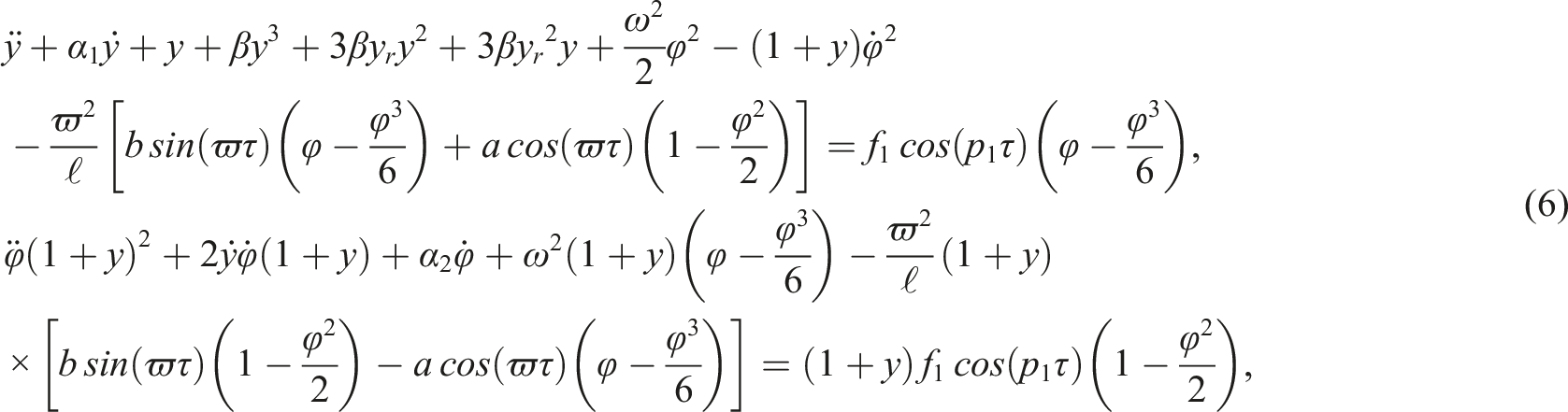
Inserting (1) and (3) in (2), to get the following EOM in a dimensionless form
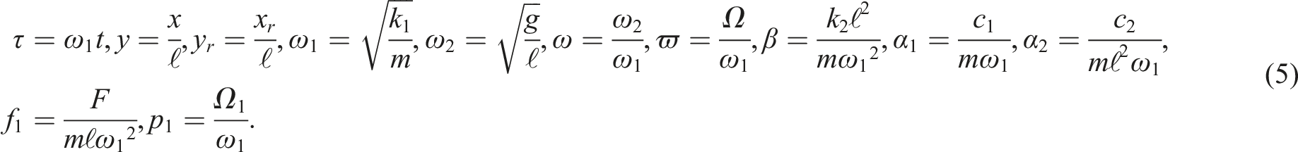
where the dot indicates the regarding differentiation with and the following dimensionless parameters are furthermore present
The proposed method
Consider checking the oscillations of the system near the position of static equilibrium. Then, functions and may be roughly calculated using Taylor’s series up to third order. Consequently, equations (4) are rewritable in the form
next, a small parameter is used to represent the coefficients of damping, amplitudes of forces, and the ellipse’s semi axes, as follows
It is assumed that the oscillations' amplitudes are of order of , then we can express the variables and in the following form
Using MSA, the functions and can be addressed as follows9
where performs specific time scales, where is fast time scales and are slow ones. To formulate and , we can write in terms of as follows47
It is important to observe that terms of higher order than are omitted for their small size.
Substituting (7)–(10) into EOM (6) and equating the various powers' coefficients of with zero to have the following categories of differential equations
Order of ()
Order of
Order of
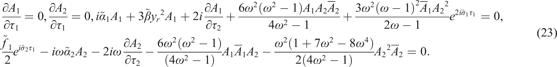
The previous equations consist of partial differential equations (PDEs) in three groups. These equations are from second order that are solvable sequentially which promote the significance of the solutions of the first group (11). Consequently, they own the below forms in their general solutions
where and are complex functions that can later be determined, and they are given as functions of slow time scales and .
Substituting (14) into (12), and then omitting the terms that lead to secular terms to avoid appearance. Therefore, we can get
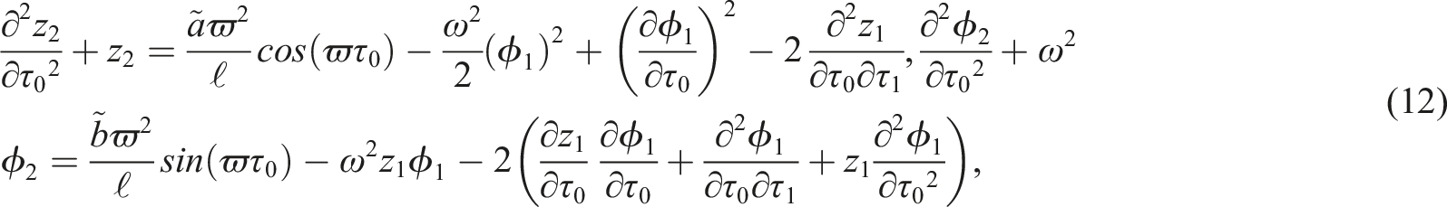
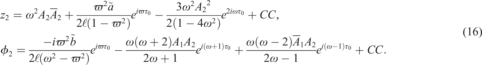
Using both of the solutions (14) and the last conditions (15), the second order’s solutions can be obtained as follows
here indicates for the preceding terms’ complex conjugate.
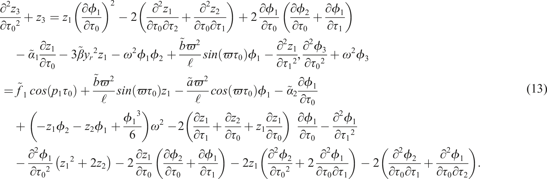
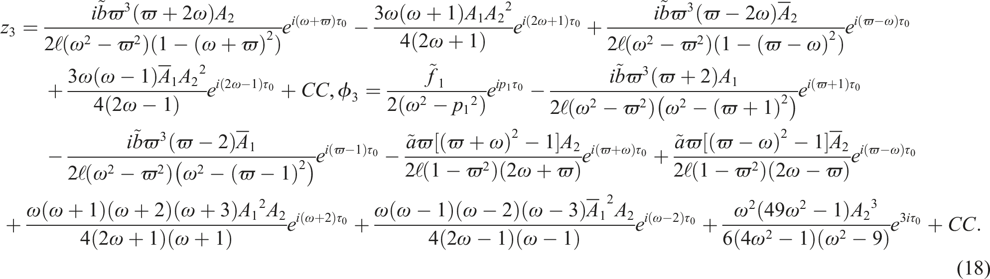
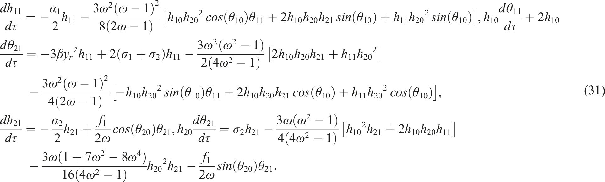
Inserting (14)–(16) in equation (13) of the third order and eliminating the secular terms to acquire the following conditions
thus, the third-order solutions possess the following forms
the unknown functions and can be specified according to the conditions of deleting secular terms (15) and (17) besides the beginning prerequisites listed below
where and are known quantities.
It must be noted that the obtained analytic solutions are fundamental to enhancing predictability, control, and performance while ensuring safety and efficiency. They provide a robust framework for understanding and managing the behavior of complex systems, leading to advancements across multiple fields and technologies. Here are some key benefits:
Knowing the solutions allows engineers to design systems that operate within desired parameters, avoiding resonant frequencies that could lead to excessive vibrations and potential failure. The obtained outcomes enable the development of control strategies to maintain desired motion patterns, enhancing system performance and safety. Stability analysis of these solutions helps in identifying safe operating conditions, ensuring that the system remains within stable regions under varying loads and disturbances. In mechanical systems, operating at such solutions can minimize energy consumption by reducing unnecessary or chaotic vibrations. In applications like automotive and aerospace engineering, understanding and controlling solutions help reduce noise generated by mechanical vibrations, leading to quieter operation.
Conditions for solvability and modulation equations
The obtained analytic solutions are acceptable when their denominators have non-zero value, that is, when the vibrations escape from resonance cases.24 These situations arise whenever one or more of the denominators in the second and third approximations equals zero. So, the detected resonance can be selected as follows:
• When is met, primary (main) external resonance takes place.
• When and are realized, the case of internal resonance is presented.
• At , combined resonances are obtained.
If one of the aforementioned resonance situations is satisfied, the behavior of the system under investigation will be highly challenging. Then, we must modify the technique being used.
We’ll look into primary external and internal resonances that happen simultaneously in order to address this state. As a result, we consider the occurrence of the following two situations at once:
These relations show how near and are to and . To fulfill this purpose, introducing dimensionless amounts is required. They are known as detuning parameters and (which specify how far vibrations are from the strict resonance) in the way
Then, we may assume they are of as following
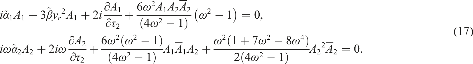
Let us substitute (21) and (22) into (12) and (13), then eliminate terms that give secular ones to have the conditions of solvability for the second and third orders as follows
The preceding solvability conditions distinguish that they are generating a system of four nonlinear PDE regarding with the undetermined functions and . Furthermore, the functions are depending upon the scale only, as obvious from condition (23). For this reason, these functions are presented in a polar form as follows
where and express the phases and amplitudes of the solutions and , respectively, in which they are real functions.
The simulations above allow us to rewrite derivative operators of the first order for and in the following ways
The PDE (23) can be transformed into ordinary differential equations (ODEs) using the formula (25). Inserting (24), (25), (8), and (10) in addition to the next adjusted phases
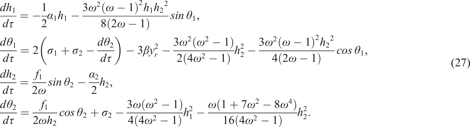
into (23), by detaching the real and imaginary parts. It is easy to get the below autonomous system of ODE regarding to and
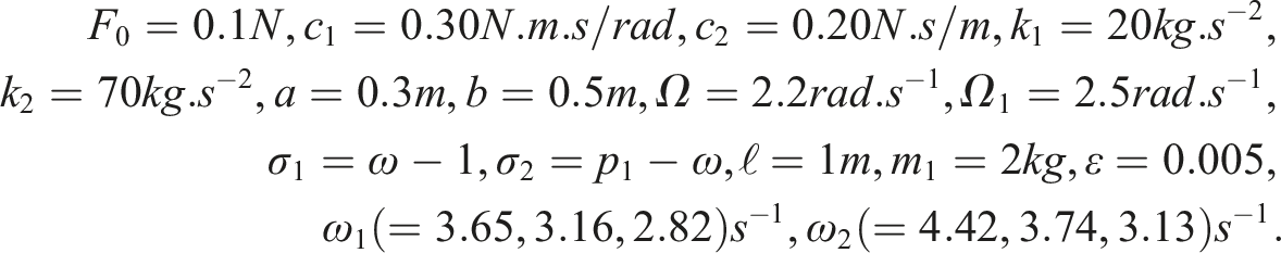
The above equations are known by the equations of modulation for the amplitudes and adjusted phases , where it is made up of four first-order ODEs that can be gained when two resonance cases happen at once. Based on the below data, these equations are solved numerically, to show their behaviors at certain values of the parameters of the system, as seen in Figures 2–7
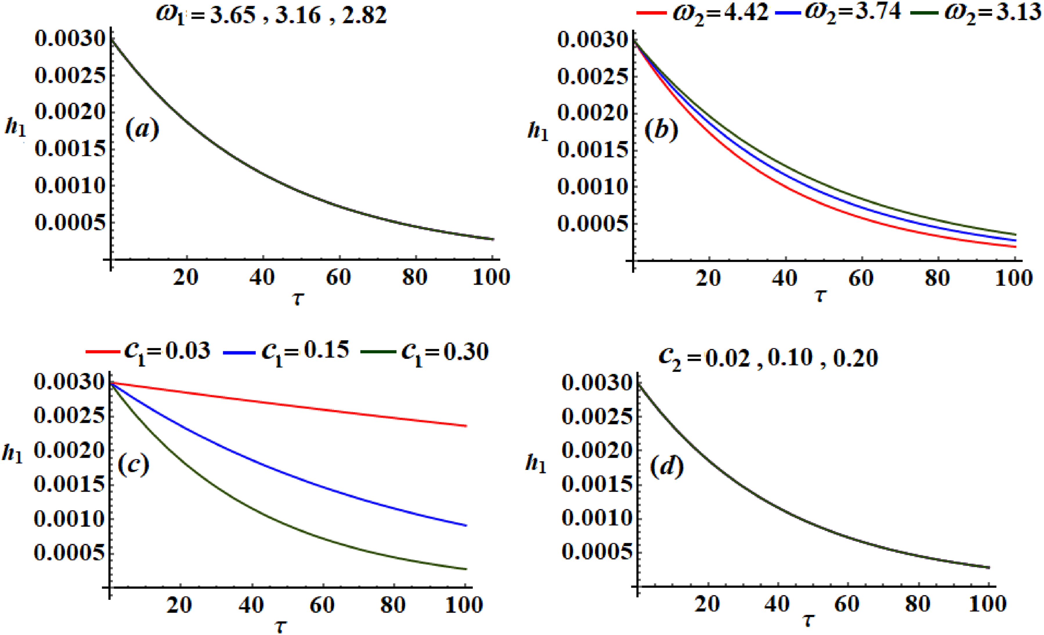
to examine the importance of the used parameters on the behavior of dynamical systems, Figures 2–7 are sketched to present the transient responses of the adjusted amplitudes and phases at specified values of the frequencies . These values line up with the pendulum arm’s typical length , the damping coefficients , and the mass , as graphed in portions of these figures. Curves of them are decaying with , which express their stability behavior. Figure 2 plots the variation of with time when and have the values and , respectively. According to the mentioned different values of parameters, the variation is presented in Figure 2(a)–(d). It is obvious that the drawn curves in these figures decrease over time which is in an agreement with the first equation (27).
Variation of versus at (a) , (b) and (d) .
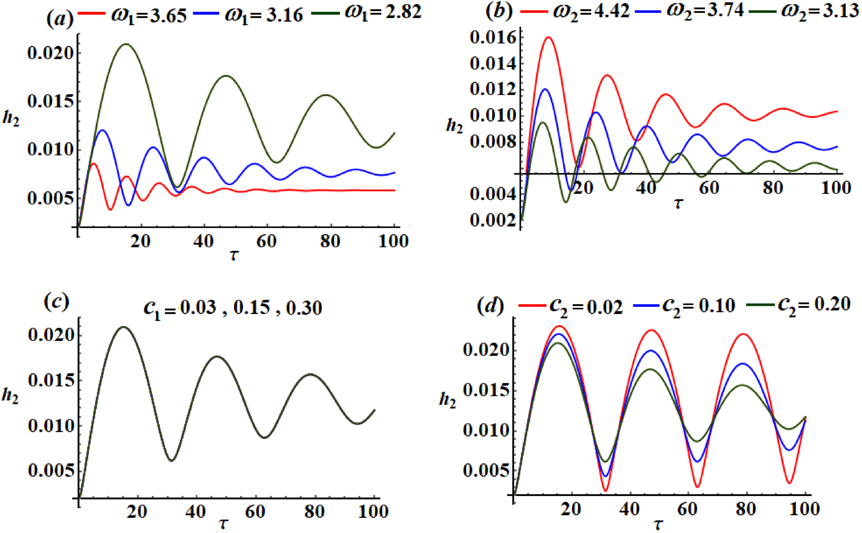
The time histories of at distinct values of and .
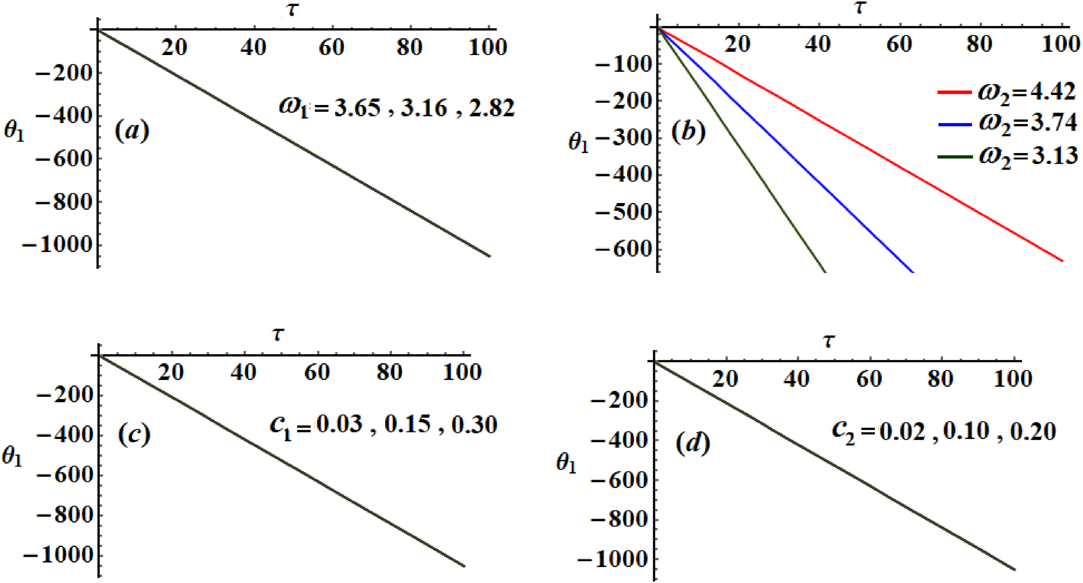
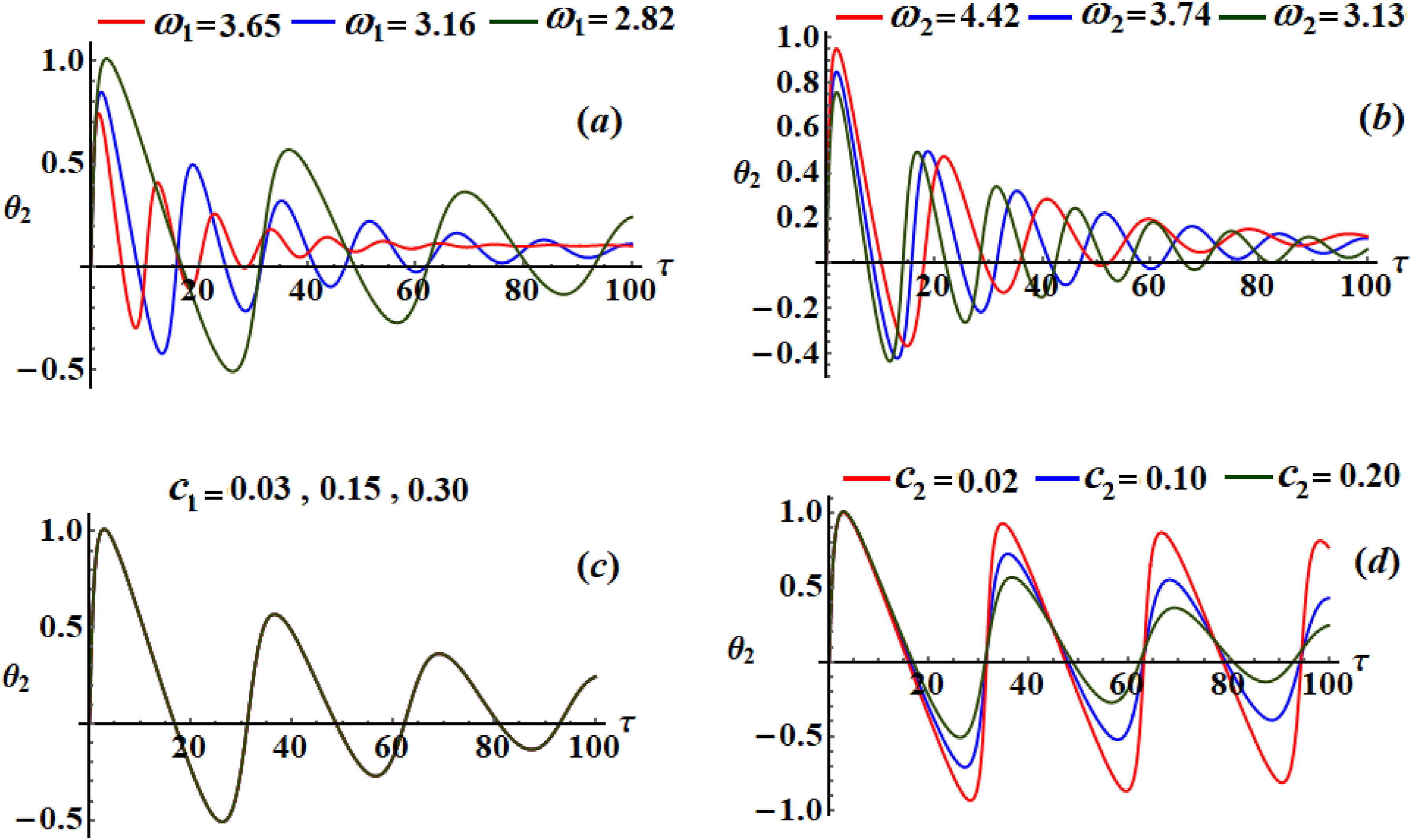
Phase (a) when (b) when (c) when and (d) when .
Displays for various values of and .
Curves in the plane at selected values of and .
Phase plane curves for distinct values of and at (a) (b) (c) and (d) .
Examining the indicated curves in Figure (3) reveals that when and have the various selected values mentioned above, the amplitude changes with . Generally speaking, the values of these parameters affect the way that all drawn waves decay, and we can note that if increases, the amplitude of wave increases and the number of oscillations decreases, on the contrary, the performance of . The plotted curve in portion (c) shows that the change of the damping coefficient doesn’t affect the behavior of the amplitude . We may see in portion (d) of the same figure that when the coefficient of damping increases, the amplitude of decreases while the oscillations’ number remains steady.
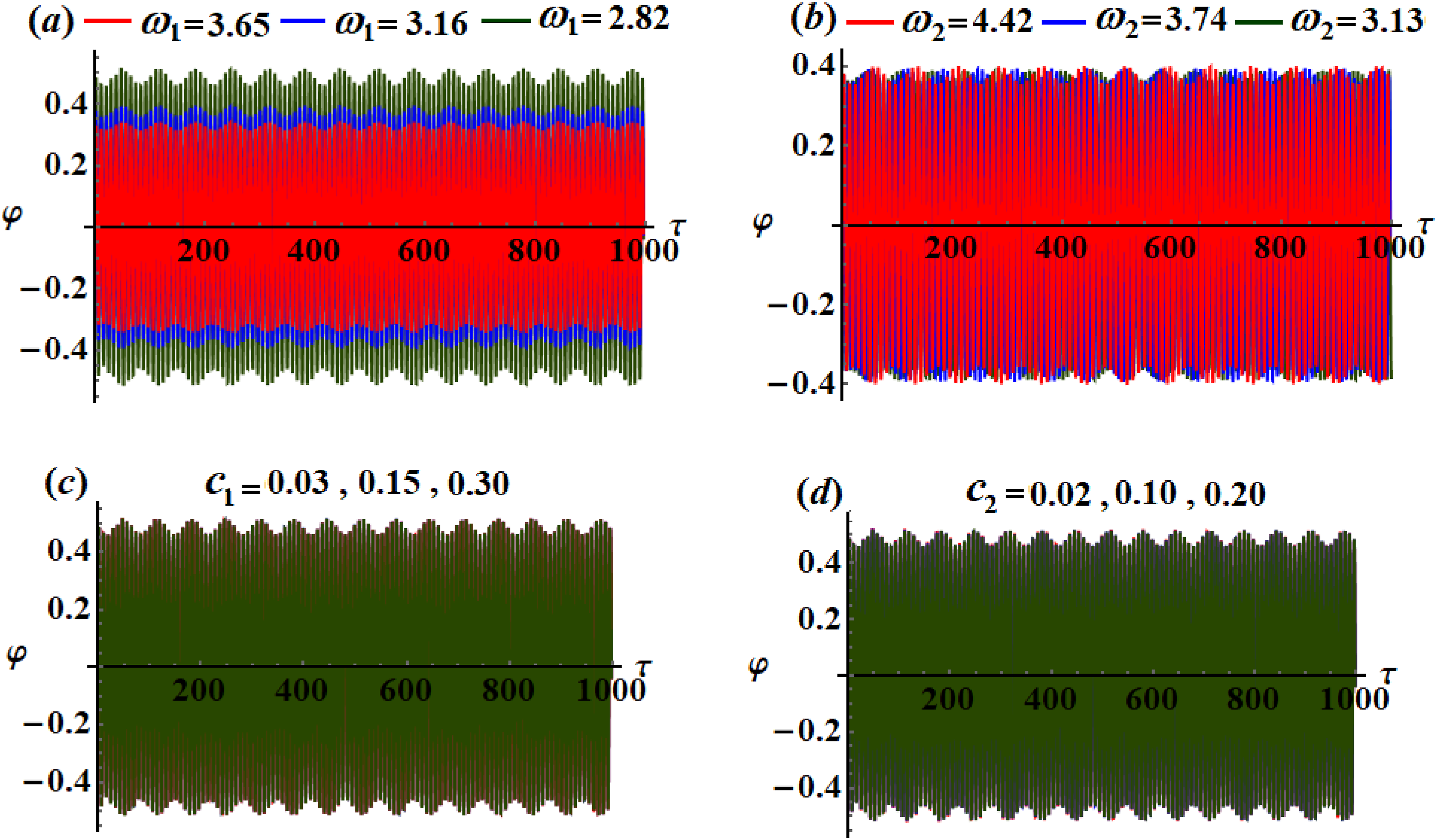
On the reverse side, Figures 4 and 5 show the time change of the adjusted phases when and have distinct values. It is observed that value changes have a negligible effect, as graphed in Figure 4(a), (c), and (d), while this alteration is progressively obvious with various values of , as indicated in Figure 4(b). The behavior of waves has a positive impact with change of the values of and as explored, respectively, in the parts (a), (b), and (d) of Figure 5. However, has no variation, to some extent, with the values of , as explored in Figure 5(c). The reason is owing to the first and fourth equations of system (27), in which the last equation doesn’t depend explicitly on , while it depends upon directly, as seen in the dimensionless parameters (5).
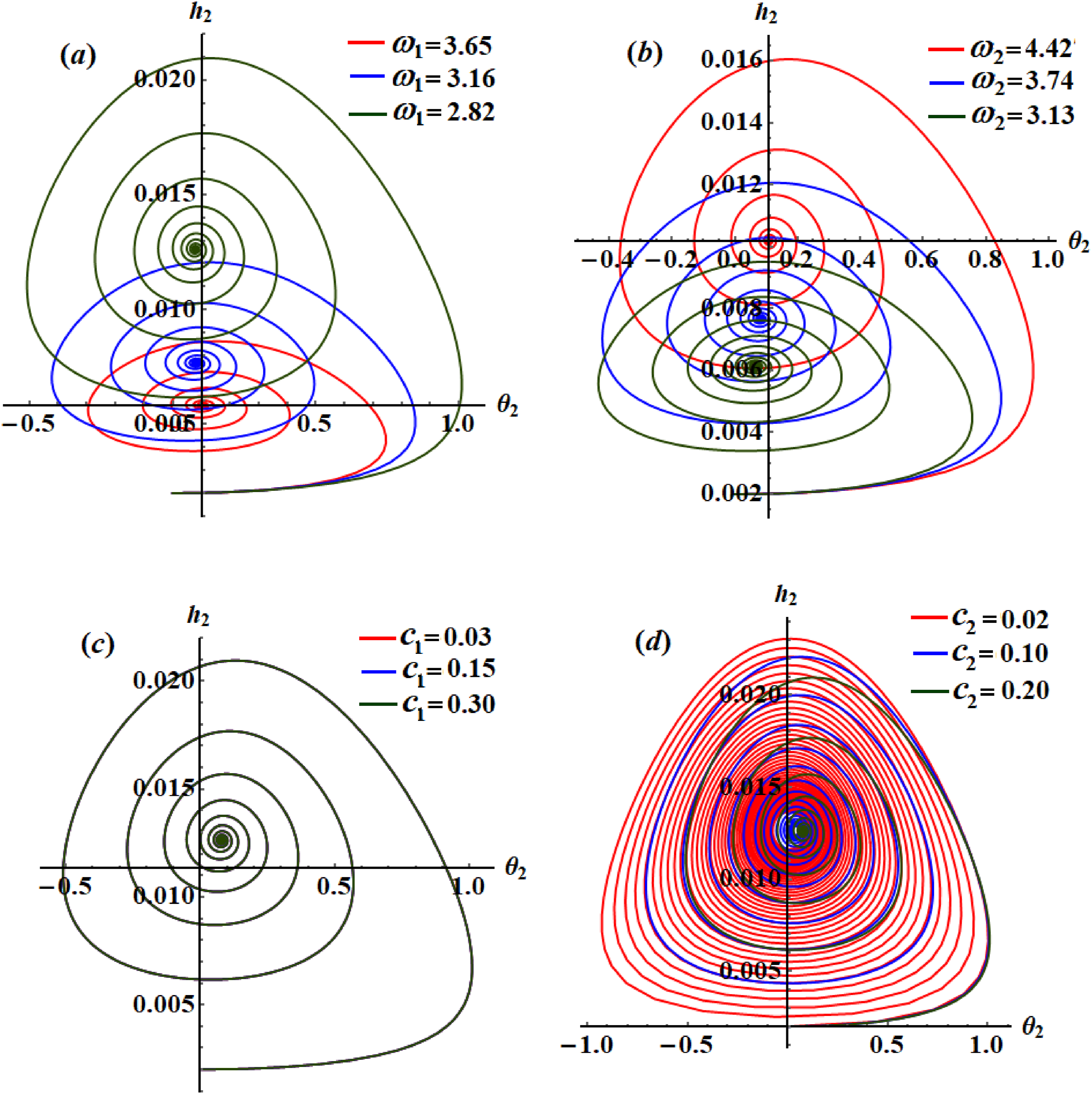
Figures 6 and 7 display the phase plane charts of the amplitudes and the adjusted phases for different values of and . It is significant to note that the drawn curves in the plane have a decaying behavior with time, in which and have a positive impact on these curves, as graphed in Figure 6(b) and (c). Curves in Figure 6(a) and (d) don’t vary with the changes of and . The inspection of the curves of Figure 7 reveals spiral arcs pointing in one direction, which demonstrates the stability of these amplitudes and phases. The sensitivity of the dynamical system (17) to the chosen values and is much higher than the value of , as seen from the plotted curves in Figure 7.
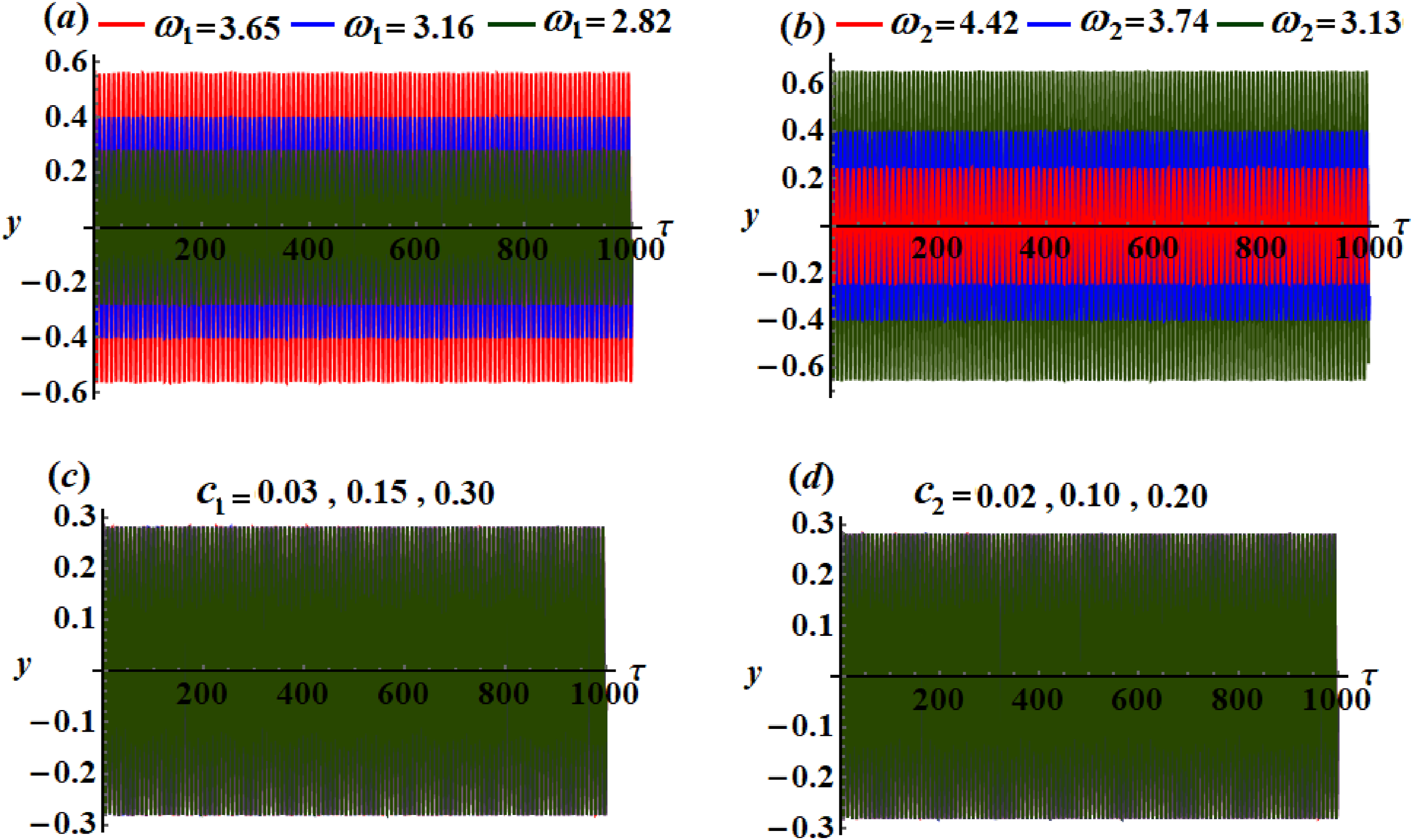
In Figures 8 and 9, the approximate solutions and through time have been drawn to represent the time-historical behavior pertaining to these solutions. These figures were computed using earlier data.
Temporal time behavior of when and vary.
Impact of changing and on the solution .
In Figure 8, the variation of the rotation angle is described as time passes, while Figure 9 displays the variation of spring’s extension with time when the parameters being utilized are the same values. Look at the graphs in portions of Figure 8, where it is evident that as rises, the plotted waves having periodic forms and their amplitudes decrease, as seen in portion (a), while portion (b) reveals decrease of the amplitude, to some extent, when increases. On the other hand, Figure 9(a) demonstrates a reduction in wave amplitudes when decreases, whereas an increment of the wave amplitudes is found in Figure 9(b) with the raise of values. The change of the approximate solutions with the values of and seems slightly, as represented in portions (c) and (d) of Figures 8 and 9. According to these curves, the solutions are considered to be stable
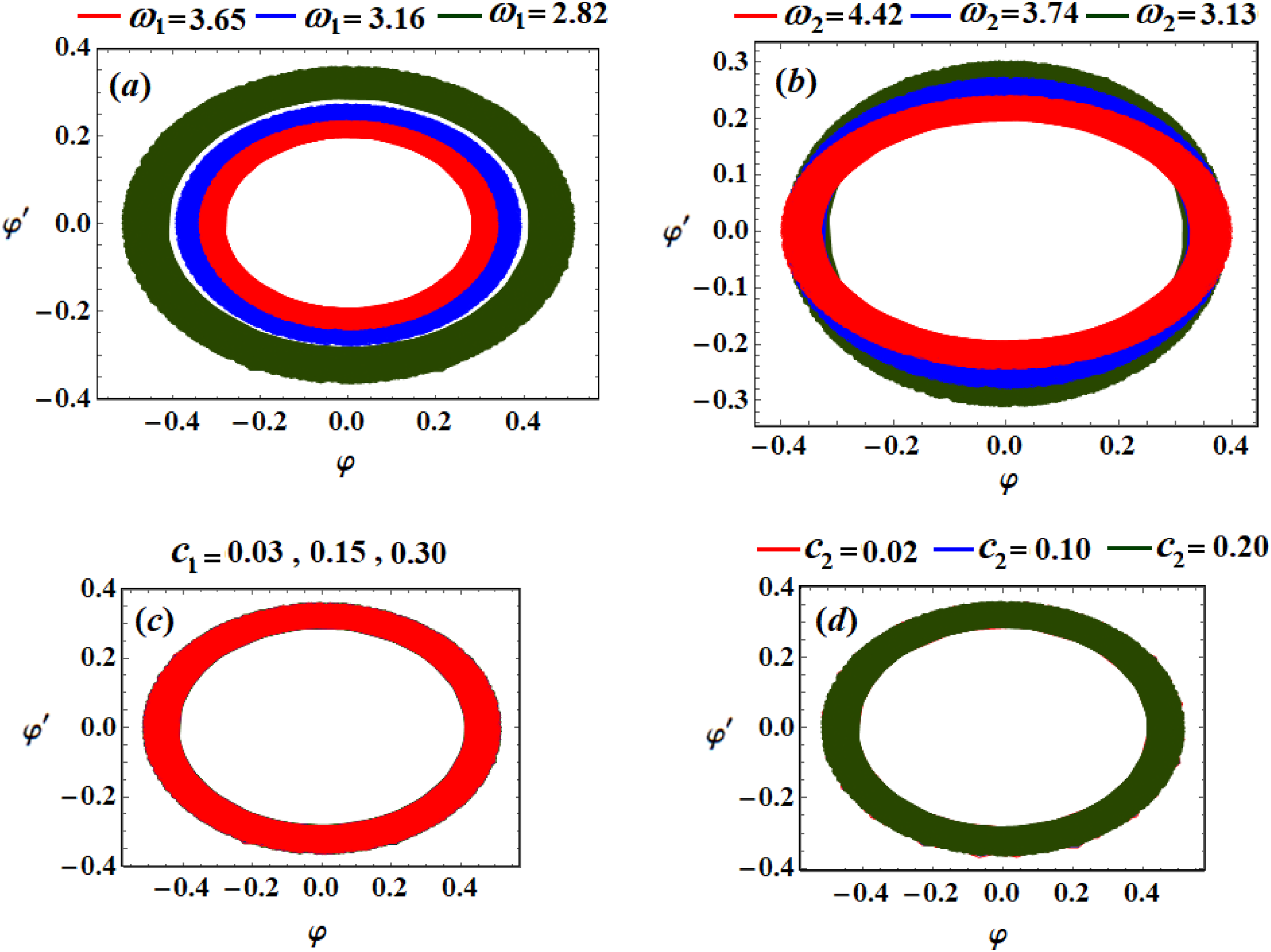
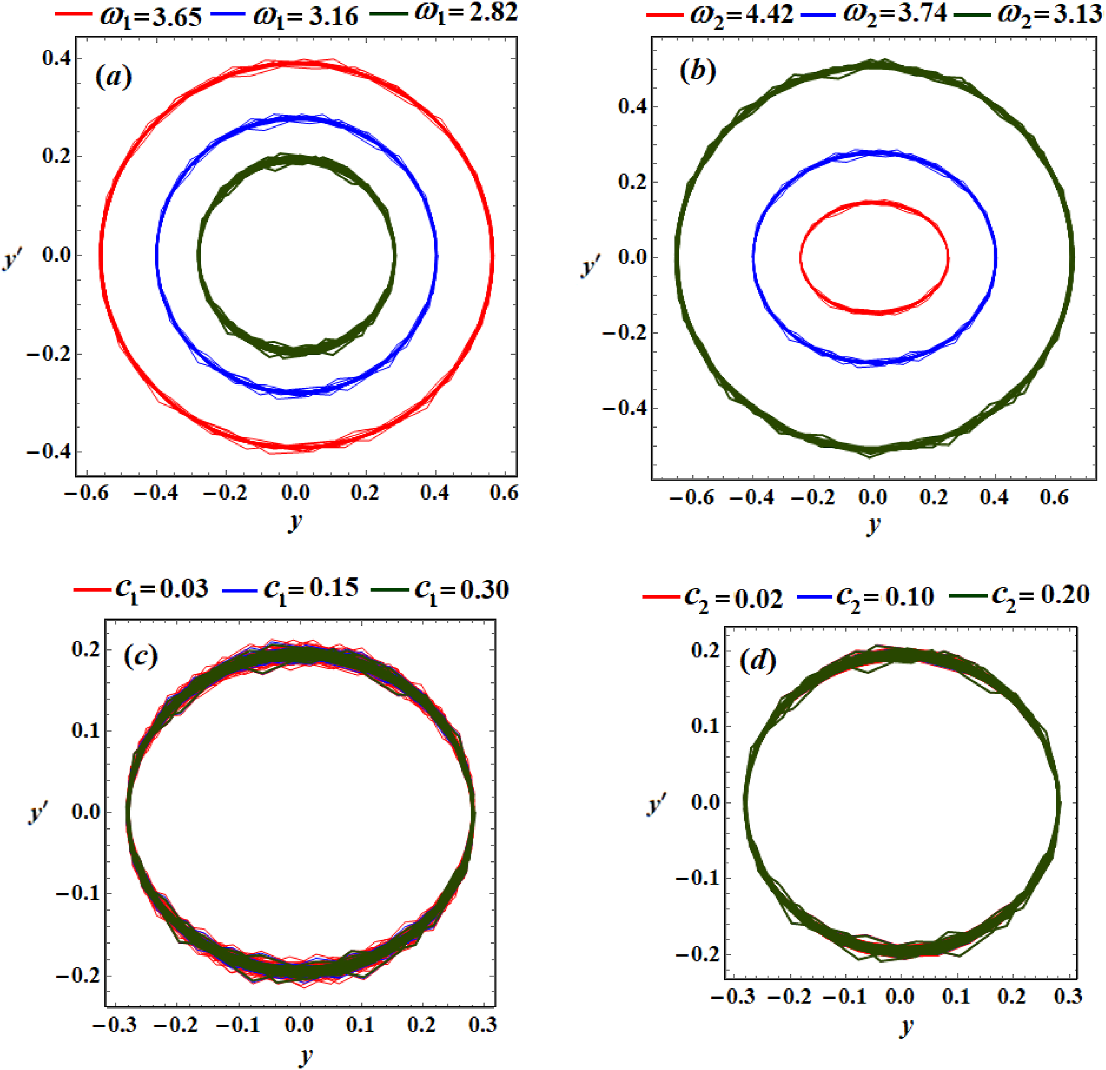
Finally, Figures 10 and 11 display the trajectory projection of the modulation system on the phase plane and . These waves are obtained at different parameters and , respectively, in which their curves have closed forms, that are consistent with the aforementioned discussion and assert the stability of the obtained solutions.
Curves’ phase plane of at the considered values of and .
Curves’ phase plane of at the considered values of and .
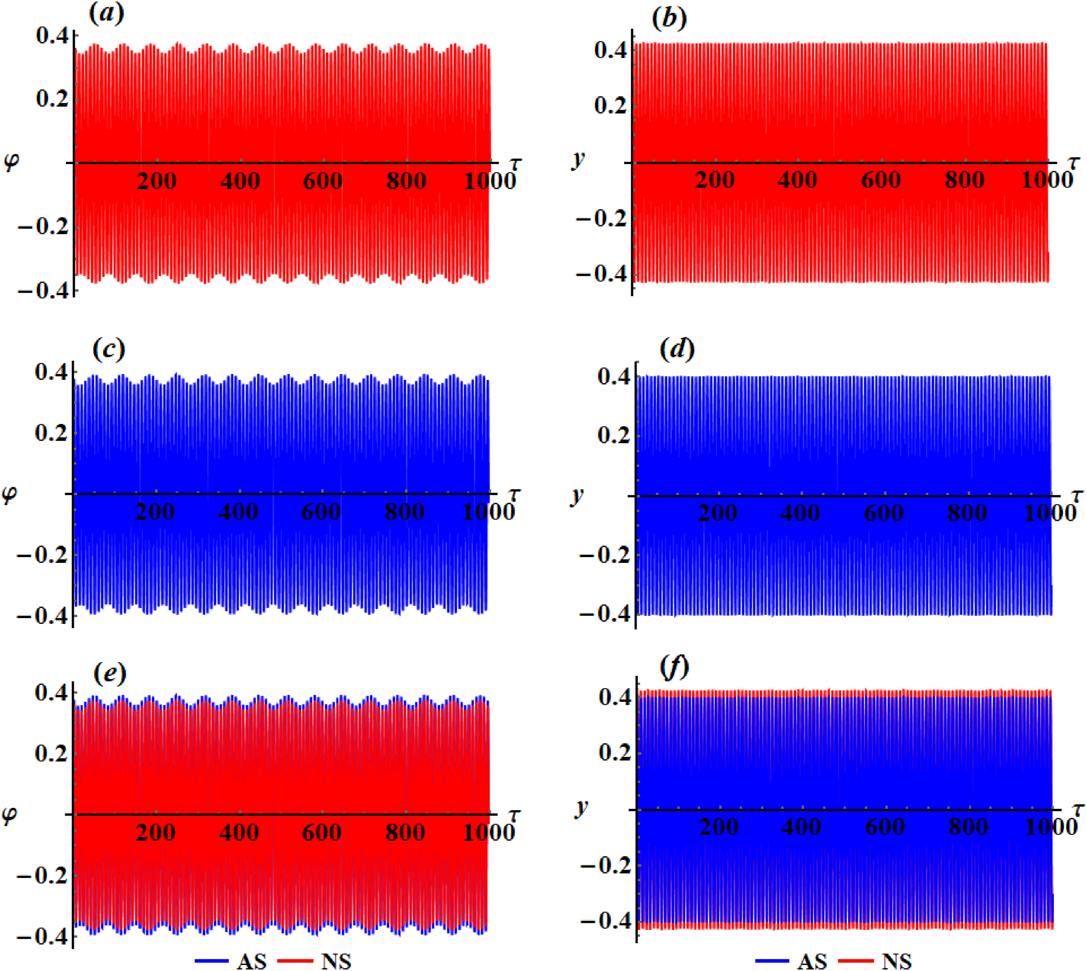
The algorithm of fourth-order Runge–Kutta is applied to gain the numerical solutions (NSs) of the basic EOM. They are graphed at in Figure 12(a) and (b) for the solutions and , respectively. On the other hand, the corresponding analytical solutions (ASs), are drawn for the aforementioned parameters in Figure 12(c) and (d). Figure 12(e) and (f) show a comparison between the NS and AS that demonstrates their great compatibility which demonstrates that the utilized perturbation approach is accurate.
Comparison between the AS and NS at and .
Steady-state solutions
The purpose of this section is to look the oscillations of the examined dynamical system at the scenario of steady-state. In general, steady-state oscillations will be produced when transient processes terminate under the impact of dampening. The amplitudes and adjusted phases of steady-state may be attained in light of zero values of the system (27), that is, at Thus, we are able to write
This system is composed of four algebraic equations that are expressed in terms of the amplitudes and adjusted phases . When the modified phases are considered to be absent, system (28) generates two nonlinear algebraic equations between the amplitudes and the parameters of detuning , as follows
It is important to note that and represent, respectively, the amplitudes of the longitudinal and swing oscillations.
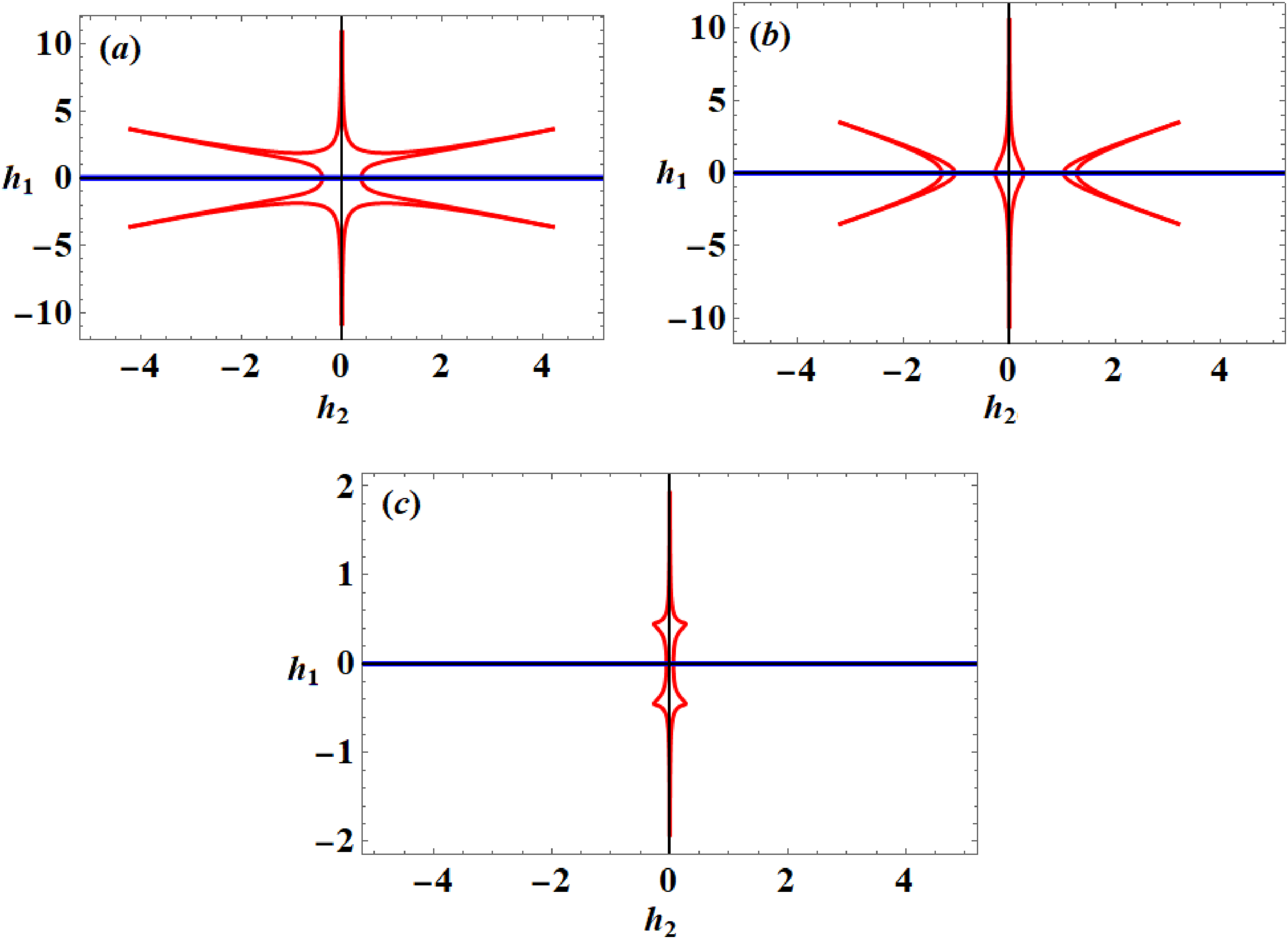
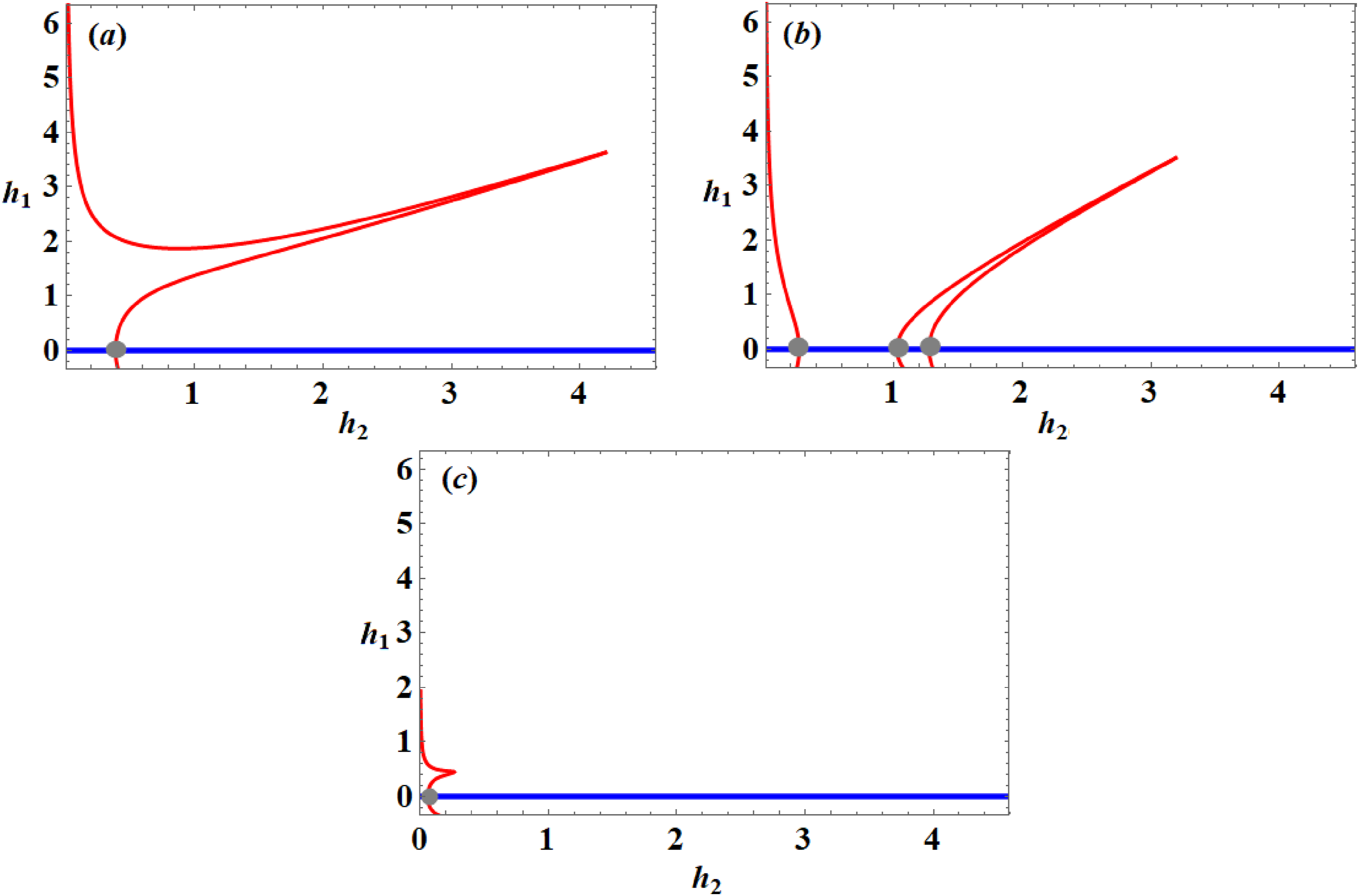
In light of the equations of system (29), the stability of the FP can be assessed. Therefore, curves of Figure 13 are plotted in the plane at and . The intersection of these curves generates FP, in which they are zoomed and marked by small gray circles, as in Figure 14. Figure 14(a) and (c) contain one unstable fixed point, which doesn’t satisfy all the conditions of (34), while three unstable FPs are indicated in Figure 13(b).
To accomplish the system’s performance in a region that is quite near the FP, consequently, the following expressions of and are taken into consideration in the system (27)
here and represent the solutions at the scenario of steady-state, while and denote the very small perturbations regarding and , respectively. The substitution of (30) in (27) yields the following form
Based on the unknown perturbed functions and of the adjusted phases and amplitudes, their solutions can be represented as linear superposition of where and are eigenvalues of the constants and unknown perturbation, respectively. If the solutions and are stable asymptotically, then the real parts of the roots of the below characteristic equation of (31) should be negative
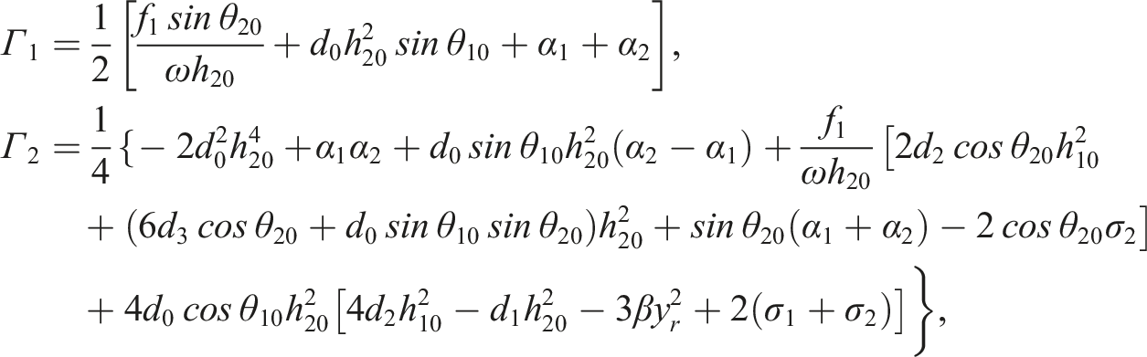
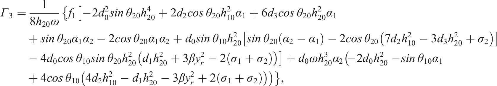
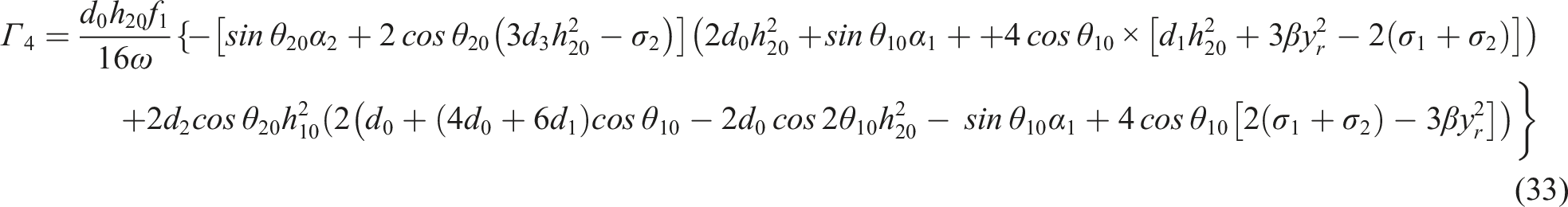
where
where
The fundamental prerequisites for stability under the RHC48 for the specific steady state solutions are
Assessment of the stability
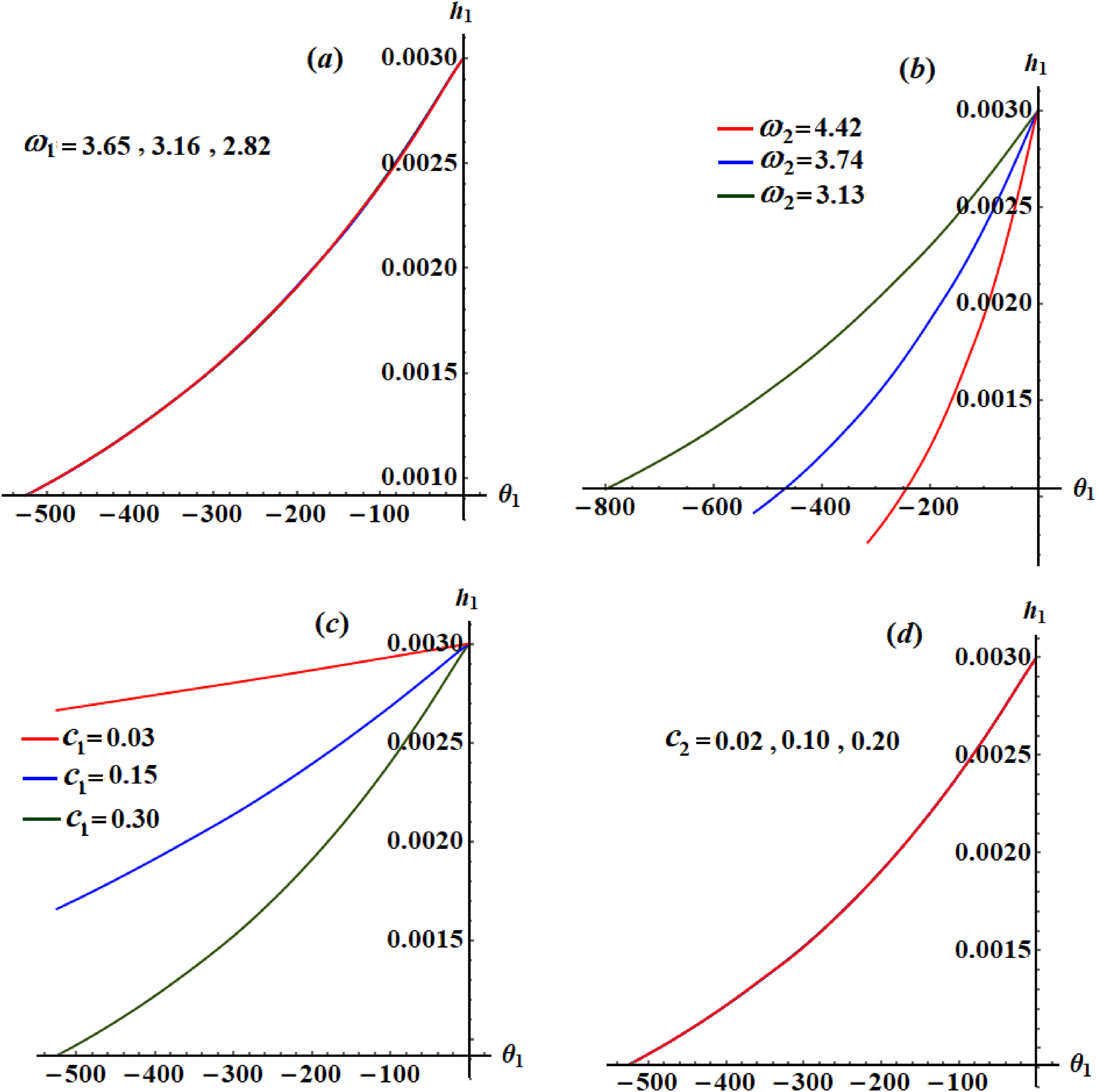
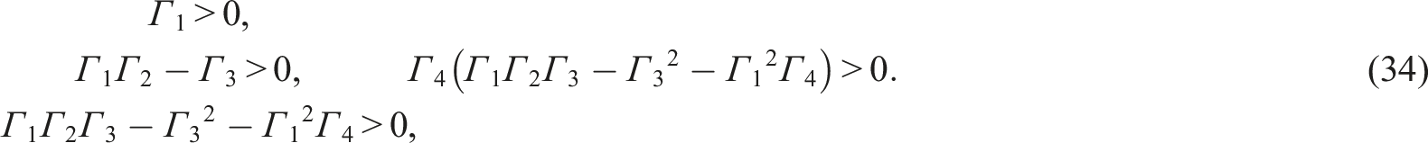
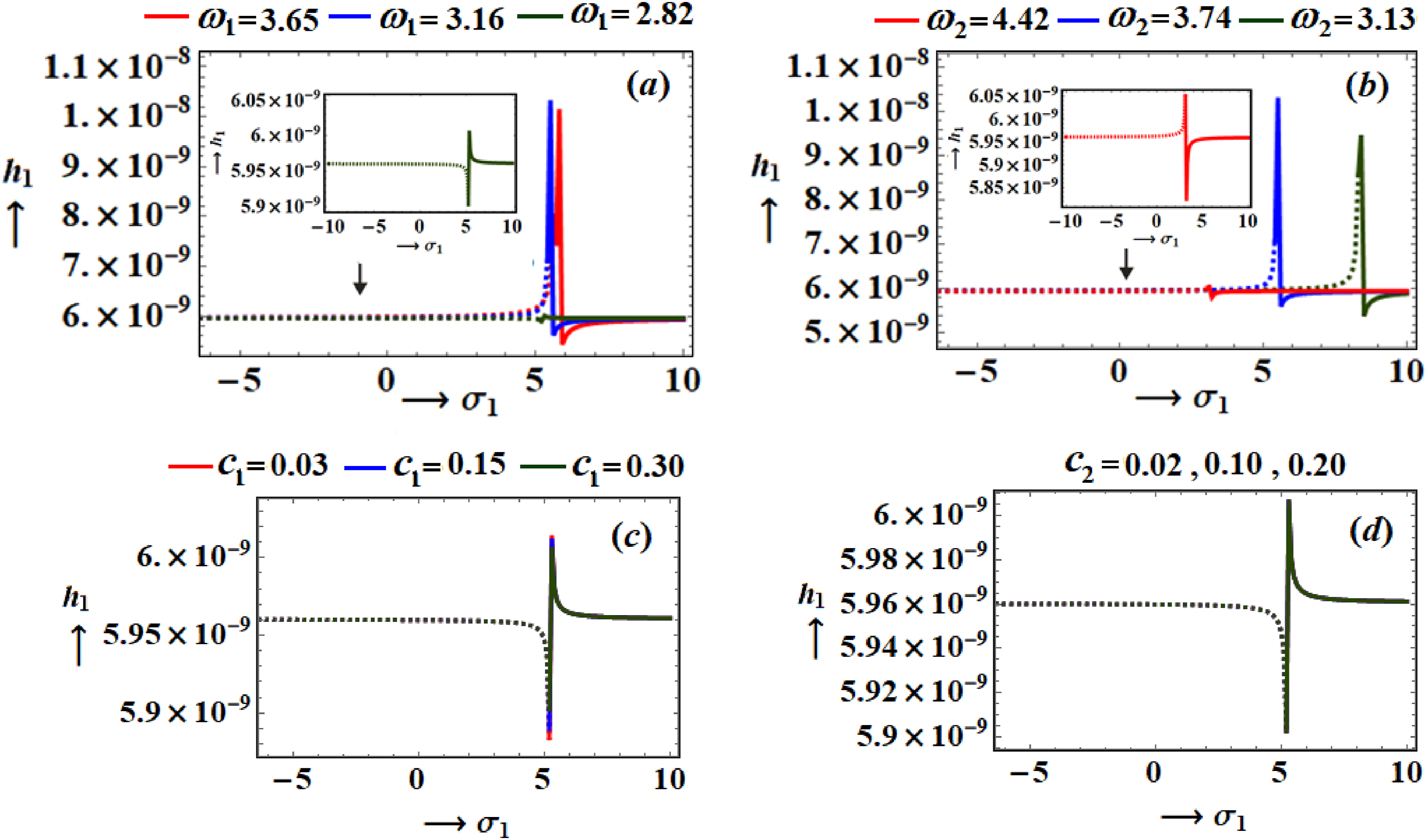
The approach of non-linear stability is applied in the present section, to study the stability of the understudied system, and both the simulation and the application of the stability parameters are included. The frequency amplitudes , detuning parameters , and damping coefficient are among the most crucial factors in the stabilization process. Considering the previously selected values for these parameters, the stability diagrams of the system (31) are plotted in Figures 15–17. For various parametrical areas, the amplitudes are displayed, and the phase plane tracks in these areas display their properties. These figures show the frequency response curves with the varying values of and . The stability/instability areas for all possible FPs are examined through the range of the curves of frequency responses. From Figure 15(a), it can be shown that, when , the stable fixed point is satisfied in the region , while the domain of unstable FP is . Similarly, the stable and unstable regions are obtained at are, respectively, , , , and . The dashed curves and the solid ones indicate the ranges of unstable and stable FPs, respectively. Each curve of this figure contains one critical point (the point between two distinct areas) and two peak points. When , the stability and instability areas have been graphed in the ranges and respectively, as seen in Figure 15(b). One critical fixed point and two peak points may be found on each curve in this figure. It should be noticed from Figure 15(c) and (d) that the possible FPs lose their stabilities in the area , while they are stable in the range .
Stability/instability regions in at when (a) .
Curves in the plane when , at the same values of Figure 15.
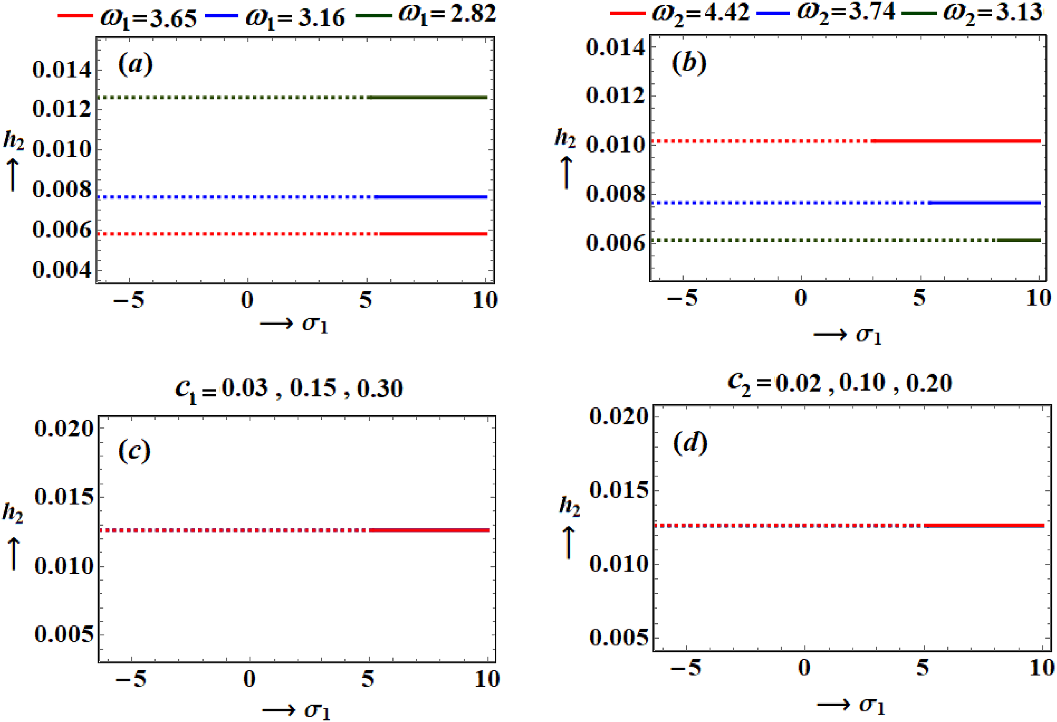
Undesired frequency response in and at when and .
Based on the previous analysis of Figure 15, we determine that the response curves in the plane have the same ranges of instability and stability FP, as drawn in portions of Figure 16. It is important to state that, when transcritical bifurcation occurs due to one fixed point, the connecting points between both curves characterize the wave’s critical values. From Figure 17(a) it is noticed that the area of unstable FP located at is , while the stable one lies in the range . One critical fixed point is observed, besides several peak ones on these curves, which it is called undesired frequency response.
Recognizing the stability and instability zones in vibrating dynamical systems yields a range of benefits across diverse applications. These include the following:
Recognizing stability zones enables engineers to design systems that function safely within these regions, reducing the likelihood of unforeseen failures. Understanding instability zones helps designers avoid parameters that cause excessive vibrations, resonance, and potential catastrophic failure. Maintaining operation within stability zones ensures smooth, efficient performance and minimizes mechanical wear. Awareness of these zones supports the tuning of system parameters for optimal performance and efficiency. Recognizing stability zones is crucial for designing effective vibration isolation systems that safeguard sensitive equipment from harmful vibrations. In structural engineering, stability analysis is applied to design buildings and infrastructure resilient to seismic activities by steering clear of instability zones that could amplify vibrations. Ensuring the stable operation of medical devices like heart pacemakers is vital for their dependable functioning.
Concluding remarks
The nonlinear planar motion of an influenced 2DOF damped elastic pendulum by harmonic force has been examined. The novelty of this work lies in the specific combination of damping, external forcing, and the elliptic path of the pendulum’s pivot point. The motion of this point is a unique aspect that distinguishes this study from other works on spring pendulums. The EOM have been obtained using Lagrangian equations. The novel analytic approximate solutions to these equations have been achieved utilizing the MSA to within three approximations. This approach helps capture the system’s behavior more accurately in the presence of nonlinearities. All resonance cases that have been detected are grouped, in which two of them are inspected simultaneously. This thorough examination of such cases adds depth to the understanding of the system’s dynamics. In line with the elimination of the secular terms, the solvability restrictions have been fulfilled, and the steady-state scenarios have been examined. These processes are considered crucial for understanding the long-term behavior of the system. The solutions' temporal trajectories, the resonance response curves, and the steady-state solutions have been displayed graphically. According to the RHC, all pertinent FPs at steady and unstable states have been located and shown. The stability zones have been looked and analyzed to determine the positive effects of various parameters, which provide practical insights for controlling and predicting the system’s responses.
Future Work
Future research could involve examining other dynamical models with 3DOF or 4DOF. More importantly, we could apply different perturbation methods to find analytical solutions. Additionally, we might model the rigid body problem as a pendulum, incorporating the movement of the support point along different paths.
Application
The examined model has gained prominence recently due to its industrial uses in seismic isolation systems for buildings and structures. In seismic engineering, a 2DOF vibrating pendulum system can be utilized as part of a seismic isolation system designed to protect buildings and infrastructure from earthquake-induced vibrations. The pendulum mechanism helps to absorb and dissipate seismic energy, reducing the amount of force transmitted to the structure. During an earthquake, the ground motion acts as an external harmonic force on the building. The distribution of mass and the structural layout can cause rotational moments that act on the building. The pendulum system can be tuned to counteract these moments, helping to stabilize the structure. The pendulum system allows for displacement in both horizontal and vertical directions, providing two degrees of freedom. This capability is essential for accommodating the complex and multi-directional nature of seismic waves.
Footnotes
Author contributions
T. S. Amer: Investigation, methodology, data curation, conceptualization, validation, reviewing, and editing.
A. A. Galal: Investigation, resources, methodology, conceptualization, validation, and writing—original draft preparation.
Declaration of conflicting interests
The author(s) declared no potential conflicts of interest with respect to the research, authorship, and/or publication of this article.
Funding
The author(s) received no financial support for the research, authorship, and/or publication of this article.
ORCID iDs
TS Amer
AA Galal
Data availability statement
All data generated or analyzed during this study are included in this published article.
References
1.
LeeWKHsuCS. A global analysis of an harmonically excited spring-pendulum system with internal resonance. J Sound Vib1994; 171(3): 335–359.
2.
LeeWKParkHD. Chaotic dynamics of a harmonically excited spring-pendulum system with internal resonance. Nonlinear Dynam1997; 14: 211–229.
3.
AmerTSBekMA. Chaotic responses of a harmonically excited spring pendulum moving in circular path. Nonlinear Anal-Real2009; 10: 3196–3202.
4.
LeeWKParkHD. Second-order approximation for chaotic responses of a harmonically excited spring-pendulum system. Int J Non Lin Mech1999; 34: 749–757.
5.
EissaMEL-SerafiSEL-SheikhM, et al.Stability and primary simultaneous resonance of harmonically excited non-linear spring-pendulum system. Appl Math Comput2003; 145: 421–442.
6.
GittermanM. Spring pendulum: parametric excitation vs an external force. Phys Stat Mech Appl2010; 389: 3101–3108.
7.
HatwalHMallikAKGhoshA. Forced nonlinear oscillations of an autoparametric system-part 1: periodic responses. J Appl Mech1983; 50: 657–662.
8.
HatwalHMallikAKGhoshA. Forced nonlinear oscillations of an autoparametric system-part 2: chaotic responses. J Appl Mech1983; 50: 663–668.
SongYSatoHIwataY, et al.The response of a dynamic vibration absorber system with a parametrically excited pendulum. J Sound Vib2003; 259(4): 747–759.
11.
WarminskiJKecikK. Autoparametric vibrations of a nonlinear system with pendulum. Math Probl Eng2006; 2006: 20.
12.
VyasABajajAK. Dynamics of autoparametric vibration absorbers using multiple pendulums. J Sound Vib2001; 246(1): 115–135.
13.
Gus’kovAMPanovkoGYVan BinC. Analysis of the dynamics of a pendulum vibration absorber. J Mach Manuf Reliab2008; 37(4): 321–329.
14.
AmerWSBekMAAbohamerMK. On the motion of a pendulum attached with tuned absorber near resonances. Results Phys2018; 11: 291–301.
15.
StarostaRKamińskaGSAwrejcewiczJ. Asymptotic analysis of kinematically excited dynamical systems near resonances. Nonlinear Dynam2012; 68: 459–469.
16.
AwrejcewiczJStarostaRKamińskaG. Asymptotic analysis of resonances in nonlinear vibrations of the 3-dof pendulum. Differ Equ Dyn Syst2013; 21 (1,2), 123-140.
17.
AmerTBekMAbouhmrM. On the vibrational analysis for the motion of a harmonically damped rigid body pendulum. Nonlinear Dynam2018; 91: 2485–2502.
18.
AmerTBekMAbouhmrM. On the motion of a harmonically excited damped spring pendulum in an elliptic path. Mech Res Commun2019; 95: 23–34.
19.
El-SabaaFMAmerTSBekMA, et al.On the motion of a damped rigid body near resonances under the influence of a harmonically external force and moments. Results Phys2020; 19: 103352.
20.
AbadyIMAmerTSGadHM, et al.The asymptotic analysis and stability of 3DOF non-linear damped rigid body pendulum near resonance. Ain Shams Eng J2022; 13(2): 101554.
21.
AmerTSStarostaRElameerAS, et al.Analyzing the stability for the motion of an unstretched double pendulum near resonance. Appl Sci2021; 11: 9520.
22.
AmerTSGalalAA. Vibrational dynamics of a subjected system to external torque and excitation force. J Vib Control2024; 0(0). DOI: 10.1177/10775463241249618.
23.
AmerTSArabAGalalAA. On the influence of an energy harvesting device on a dynamical system. J Low Freq Noise Vib Act Control2024; 43(2): 669–705. DOI: 10.1177/14613484231224588.
24.
HeJHAmerTSAbolilaAF, et al.Stability of three degrees-of-freedom auto-parametric system. Alex Eng J2022; 61(11): 8393–8415.
25.
AbdelhfeezSAAmerTSElbaz RewanF, et al.Studying the influence of external torques on the dynamical motion and the stability of a 3DOF dynamic system. Alex Eng J2022; 61(9): 6695–6724.
26.
AmerTBekMHamadaI. On the motion of harmonically excited spring pendulum in elliptic path near resonances. Adv. Math. Phys2016; 2016.
27.
StarostaRAwrejcewiczJ. Asymptotic analysis of parametrically excited spring pendulum. SYROM 2009. Berlin: Springer, 2010, pp. 421–432.
28.
StarostaRSypniewska–kamińskaGAwrejcewiczJ. Parametric and external resonances in kinematically and externally excited nonlinear spring pendulum. Int J Bifurcation Chaos2011; 21(10): 3013–3021.
29.
ZhuSZhengYFuY. Analysis of non-linear dynamics of a two-degree-of-freedom vibration system with non-linear damping and non-linear spring. J Sound Vib2004; 271: 15–24.
30.
AwrejcewiczJStarostaRSypniewska-KamińskaG. Stationary and transient resonant response of a spring pendulum. Procedia IUTAM2016; 19: 201–208.
31.
KamińskaGStarostaRAwrejcewiczJ. Two Approaches in the analytical investigation of the spring pendulum. Vib. Phys. Syst2018; 29: 2018005.
32.
BelyakovAO. On rotational solutions for elliptically excited pendulum. Phys Lett2011; 375: 2524–2530.
33.
LuoACYuanY. Bifurcation trees of period-1 to period-2 motions in a periodically excited nonlinear spring pendulum. J Vib Test Syst Dyn2020; 4(3): 201–248.
34.
AmerTSEl-SabaaFMZakriaSK, et al.The stability of 3-DOF triple-rigid-body pendulum system near resonances. Nonlinear Dynam2022; 110: 1339–1371.
35.
GhanemSAmerTSAmerWS, et al.Analyzing the motion of a forced oscillating system on the verge of resonance. J Low Freq Noise Vib Act Control2023; 42(2): 563–578. DOI: 10.1177/14613484221142182.
36.
AmerTSGalalAAAbolilaAF. On the motion of a triple pendulum system under the influence of excitation force and torque. Kuwait J Sci2021; 48(4): 1–17.
37.
LuJMaL. Analysis of a fractal modification of attachment oscillator. Therm Sci2024; 28(3A): 2153–2163.
38.
HeJHYangQHeCH, et al.Pull-down instability of the quadratic nonlinear oscillators. FU Mech Eng2023; 21(2): 191–200.
39.
NaveedAHeJH. Geometric potential in nano/microelectromechanical systems: Part I mathematical model. Int J Geomet Methods Mod Phys2024; 2024. DOI: 10.1142/S0219887824400279.
40.
JuP. Global residue harmonic balance method for Helmholtz–Duffing oscillator. Appl Math Model2015; 39(8): 2172–2179.
LuJShenSChenL. Variational approach for time-space fractal Bogoyavlenskii equation. Alex Eng J2024; 97: 294–301.
43.
LuJ. Variational approach for (3+1)-dimensional shallow water wave equation. Results Phys2024; 56: 107290.
44.
LuJ. Application of variational principle and fractal complex transformation to (3+1)-dimensional fractal potential-YTSF equation. Fractals2024; 32(1): 2450027.
45.
HeJHHeCHAlsolamiAA. A good initial guess for approximating nonlinear oscillators by the homotopy perturbation method. FU Mech Eng2023; 21(1): 021–029.
46.
MaH. Simplified Hamiltonian-based frequency-amplitude formulation for nonlinear vibration systems. FU Mech Eng2022; 20(2): 445–455.
47.
AmerTSAbdelhfeezSAElbazRF. Modeling and analyzing the motion of a 2DOF dynamical tuned absorber system close to resonance. Arch Appl Mech2023; 93: 785–812. DOI: 10.1007/s00419-022-02299-8.
48.
AwrejcewiczJStarostaRKamińskaGS. Asymptotic multiple scale method in time domain: multi-degree-of-freedom stationary and nonstationary dynamics. London: CRC Press, Taylor & Francis Group, 2022.