
Abstract
This article investigates the computational complex wave solutions of the modified Korteweg–de Vries equation combined with an adverse order of the Korteweg–de Vries model. This model was derived in 2017, where the recursion and inverse recursion operators are employed to select the integrable merged MKdV with a negative MKdV model. This integrable property is tested utilizing the Painlevé property. Verosky gave the description and properties of the opposing order recursion operator. We handle this model by implementing eleven contemporary techniques. We obtain a novel formula of complex solitary wave solutions for this model. Complex solitary wave solutions describe wave propagation, and it is also considered more mathematically concise tools to explain more details about the physical properties of models. The main goals of our paper are a comparison between these methods and introducing a novel modified method. All solutions are checked for accuracy by putting them back into the model via two different software (Maple 17 and Mathematica 12).
Keywords
AMS classification: 02.30.Jr; 02.30.Hq; 02.60.-x
Introduction
The recursion operator is regarded as a fundamental instrument in nonlinear wave theory.1–3 This operator is based on the expansion of a power series across fields and the representation of momentum. Calculating the recursion operator using the Hamiltonian is one of the techniques. The recursion operator has many features, including the following: 1. It allows writing the families of equations integrable by a given spectral issue in a compact design. 2. It supports picking up the wholesome family of the equation. 3. It is accompanied by the Hamiltonian approach of integrable equations. 4. It provides the generating operator for the family of Hamiltonian structures.
For an example of using recursion operator:
This operator is used to the KdV equation to derive all of its families and determine the family’s integrability. It is written as follows


Recursion operators are also used on the modified KdV equation, and it has the following formula
4

The modified KdV equation describes the nonlinear wave propagation in a variety of polarity-symmetric physical formations.5–7 Additionally, it defined nonlinear ion-acoustic waves as a collisionless plasma composed of adiabatic warm ions, a weakly relativistic electron beam, and non-isothermal electrons.8,9 The negative order equation is denoted by ref.
10

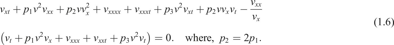
Now, combining the modified Korteweg–de Vries equation combined with an adverse order of the same models, this model has the nested formula
11

This article combines the modified Korteweg–de Vries equation with an adverse order of the same models to generate novel traveling wave solutions using over eleven recent analytical techniques.28–39
The remainder of this article is organized as follows. In Application, we applied some recent methods on the combining equation [Exp
Application
Using the next wave transformation

Exp (− ϕ(ϑ)) -expansion method
Employing Exp (− ϕ(ϑ)) -expansion method gives the following sets of the abovementioned parameters:
Set I


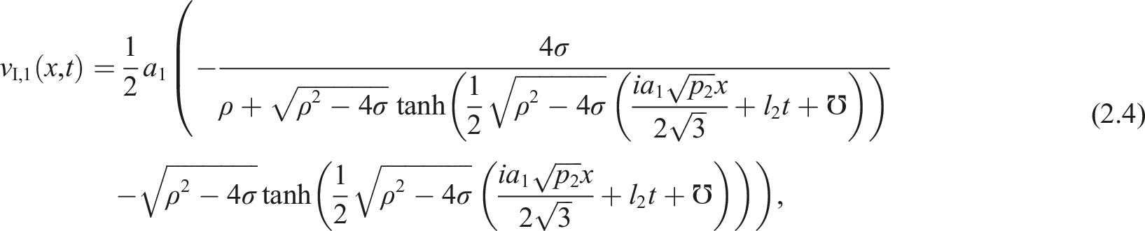
Thus, the solitary wave solutions of equation (1.5) can be formulated in the following formulas:
For ρ2 − 4σ > 0, σ ≠ 0, the solutions are given by


For ρ2 − 4σ > 0, σ = 0, the solutions are given by


Improved (G′/G) -expansion method
Employing improved (G′/G) -expansion method gives the following sets of the abovementioned parameters:
Set I

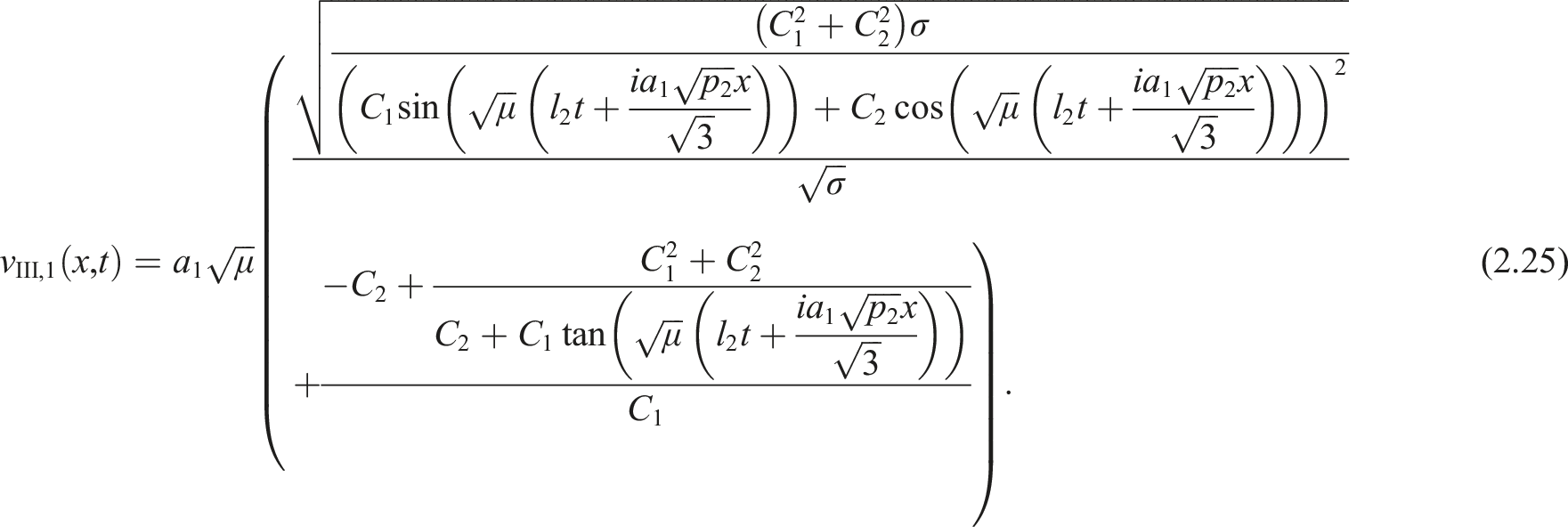
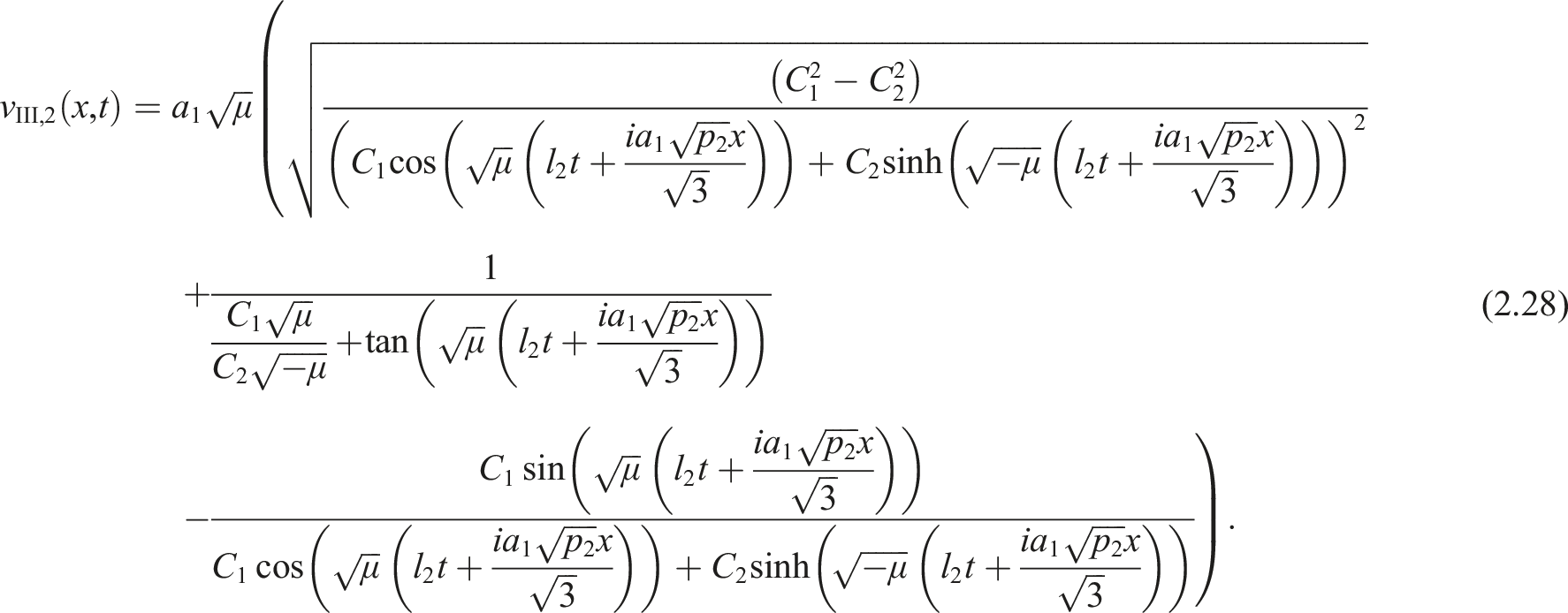
For μ > 0, the solutions are given by


Direct algebraic method
Employing the direct algebraic method gives the following sets of the abovementioned parameters:
Set I
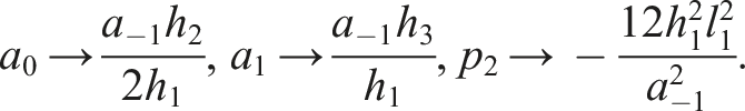
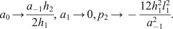
For h2 = 0, h1h3 > 0, the solutions are given by


Generalized Kudryashov method
Employing the generalized Kudryashov method gives the following sets of the abovementioned parameters:
Set I


Extended tanh-function method
Employing the extended tanh-function gives the following sets of the abovementioned parameters:
Set I
For d < 0, the solutions have been evaluated as following


Simplest equation method
Employing the simplest equation method gives the following sets of the abovementioned parameters:
Set I For c2 = − 1


Extended fan-expansion method
Employing the extended Fan-expansion method gives the following sets of the abovementioned parameters
For


For


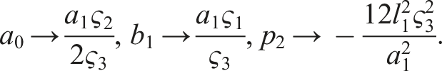
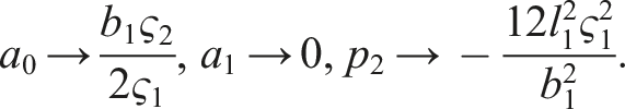
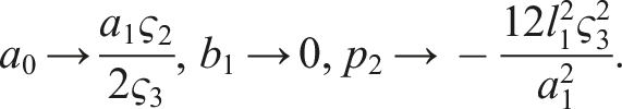
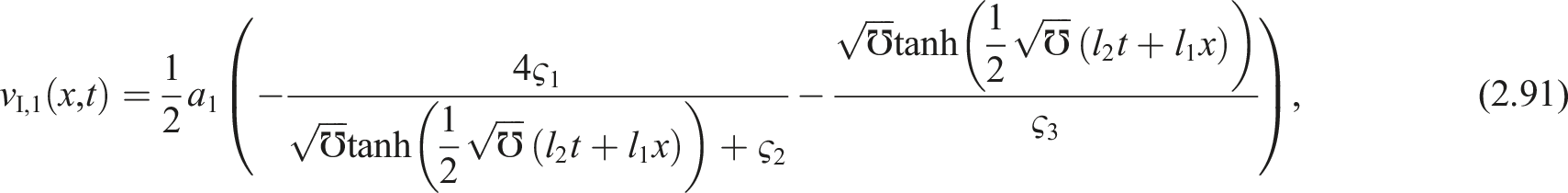
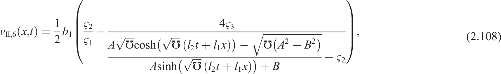
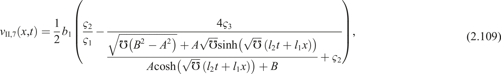
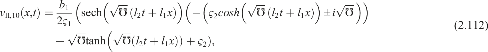
Generalized Riccati expansion method
Employing the generalized Riccati expansion method gives the following sets of the abovementioned parameters:
Set I
For


For


For


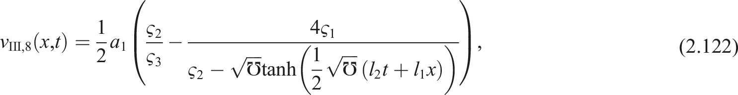
Improved F-expansion method
Employing the improved F-expansion method gives the following sets of the abovementioned parameters:
Set I


For ϱ < 0, the solutions have been evaluated as following


Generalization sinh-Gorden expansion method
Employing the generalization sinh-Gorden expansion method gives the following sets of the abovementioned parameters:
Case
Set I


Set A


Modified Khater method
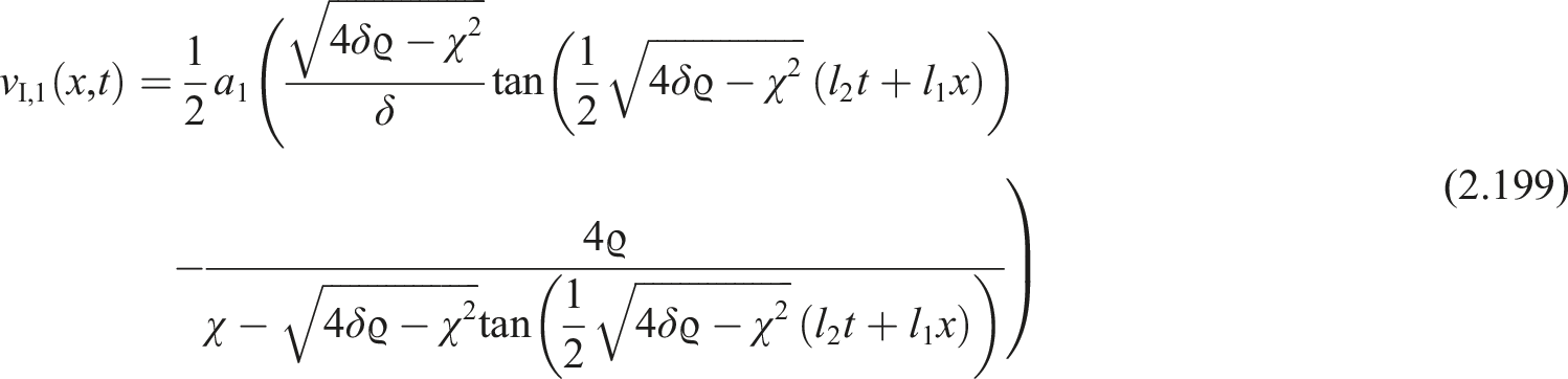
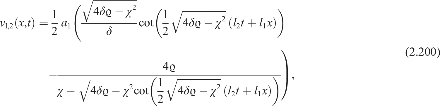
Employing the modified Khater method gives the following sets of the abovementioned parameters:
Set I
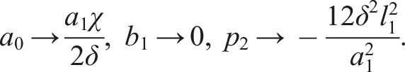
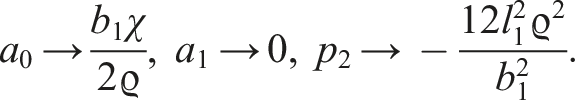
For χ2 − 4δϱ < 0, δ ≠ 0, the solutions are given by


Result and discussion
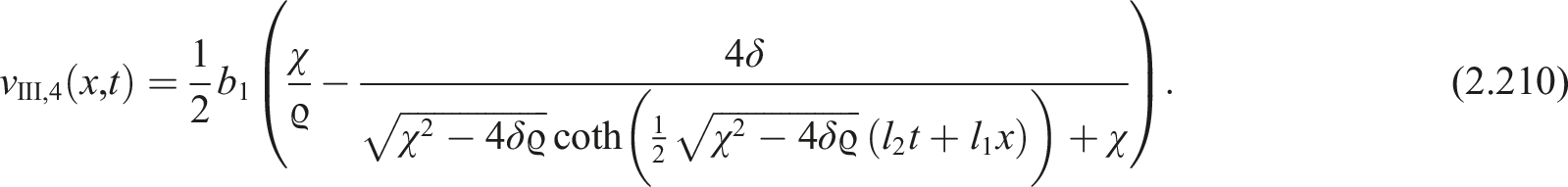
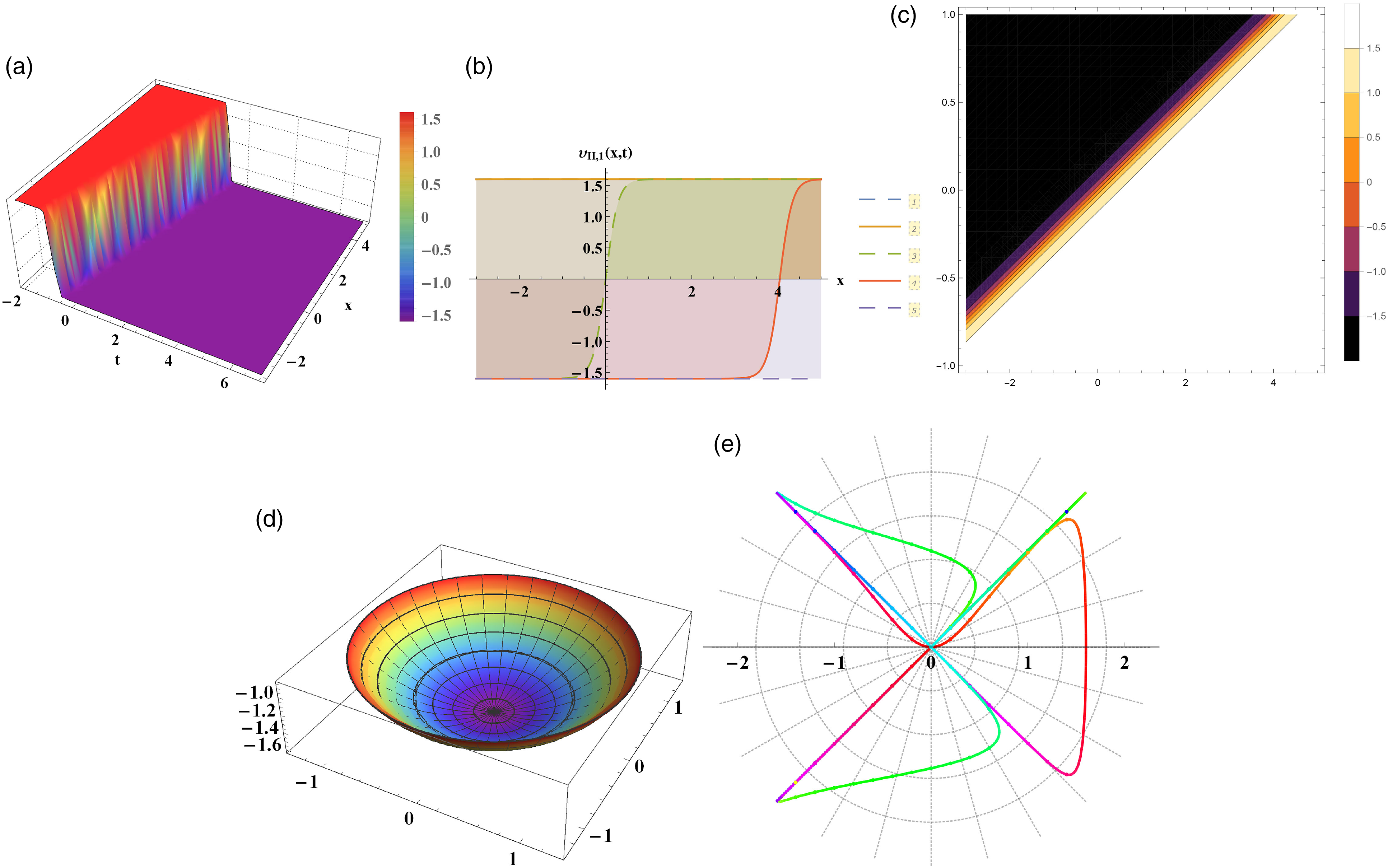
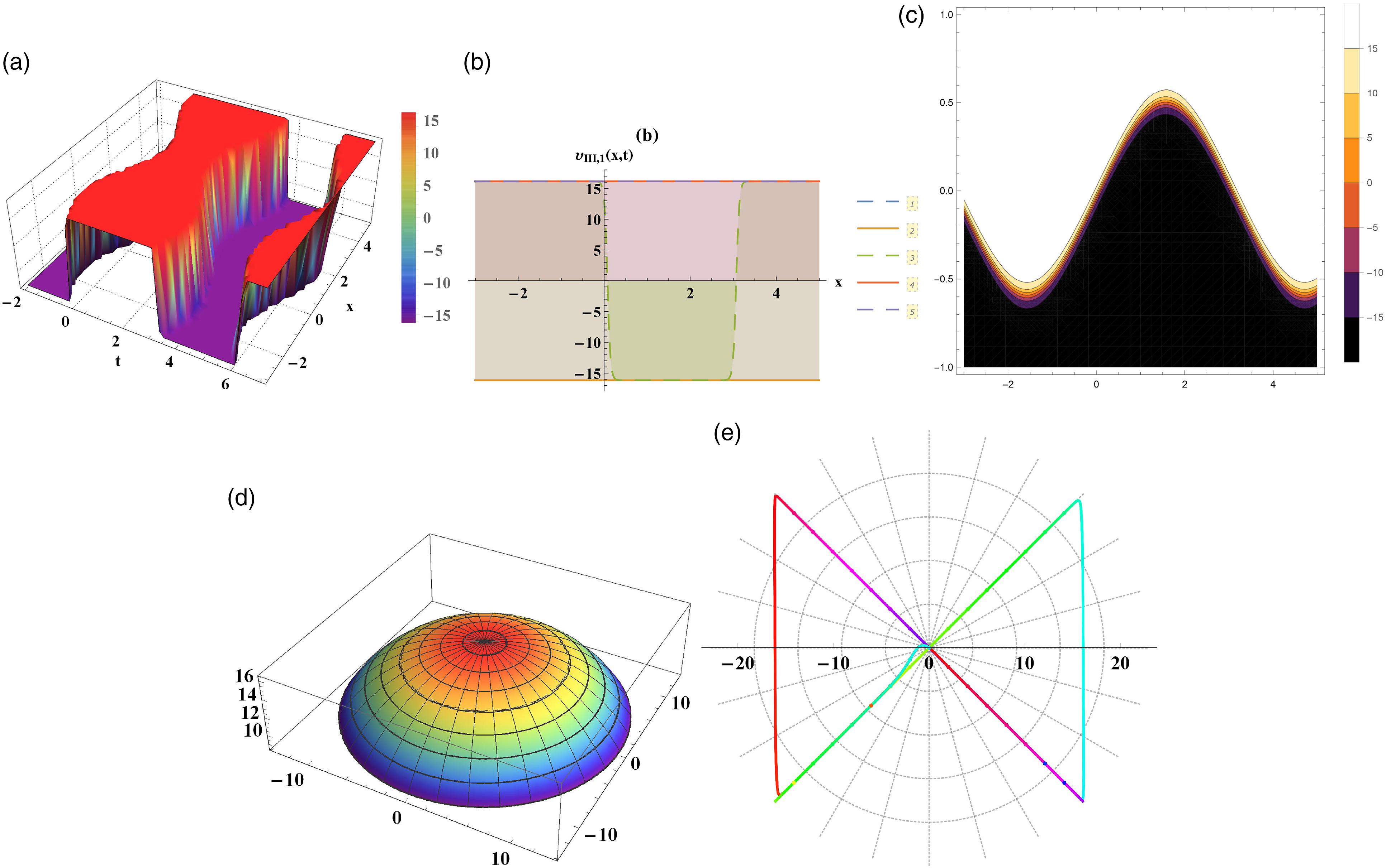
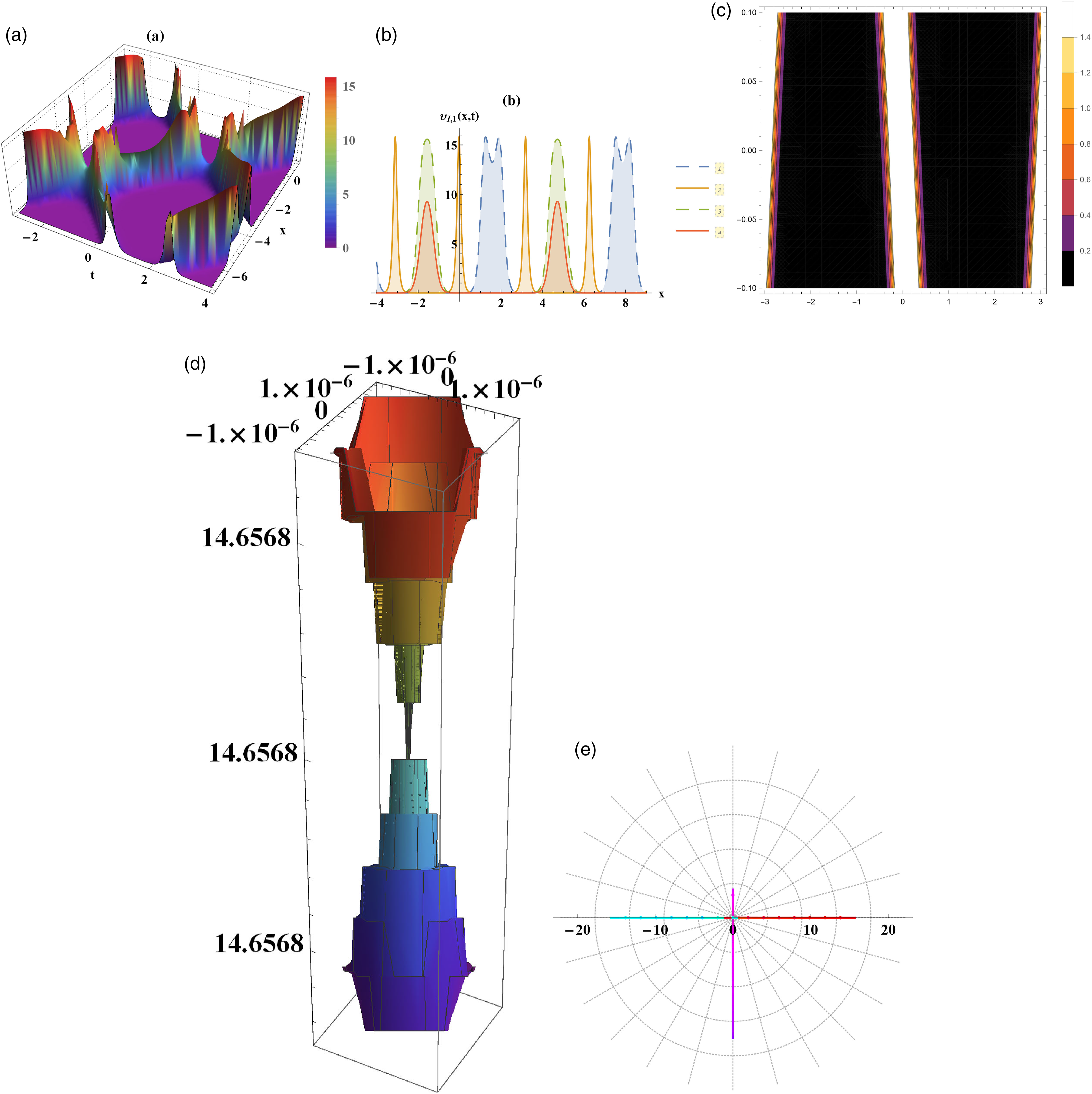
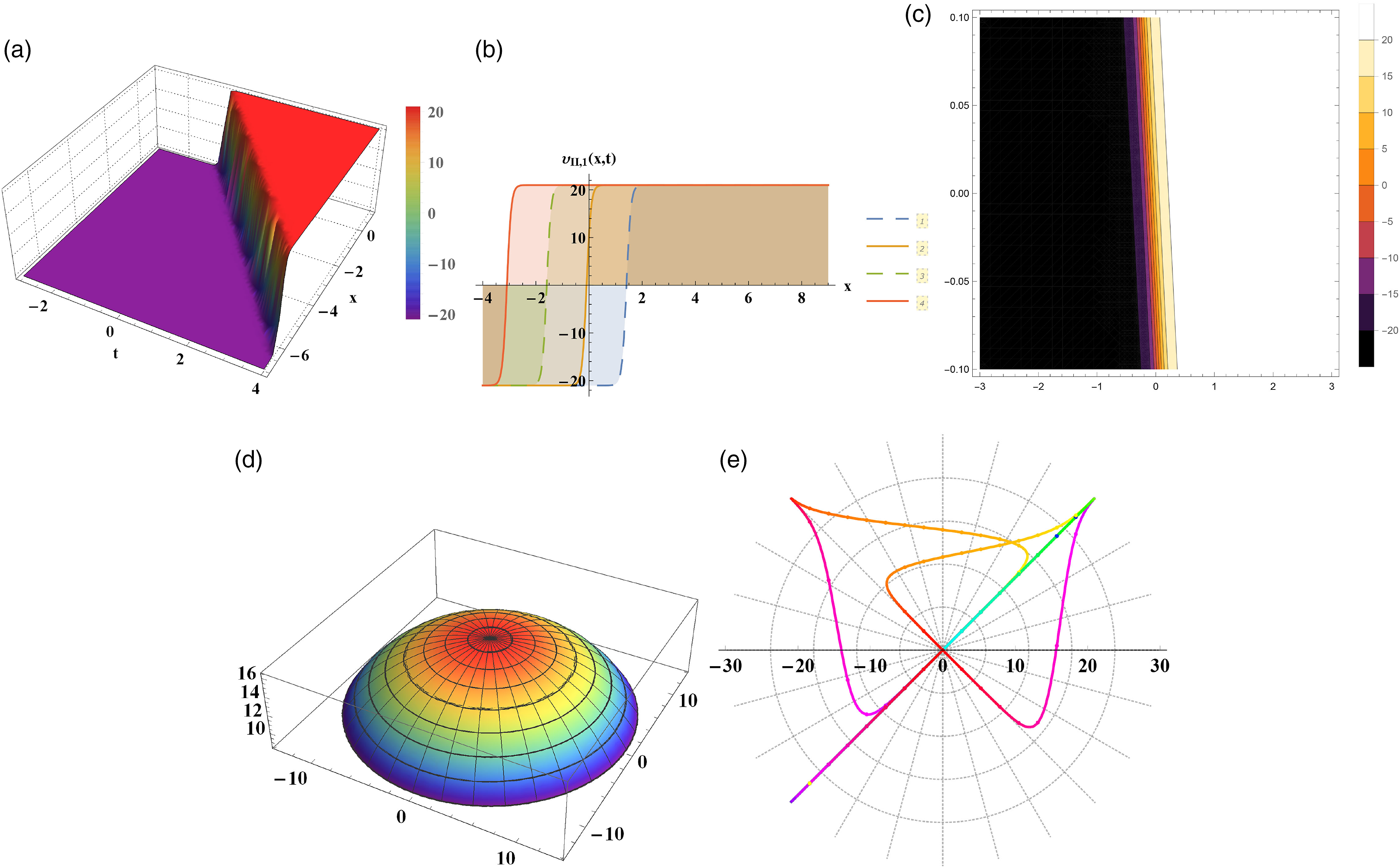
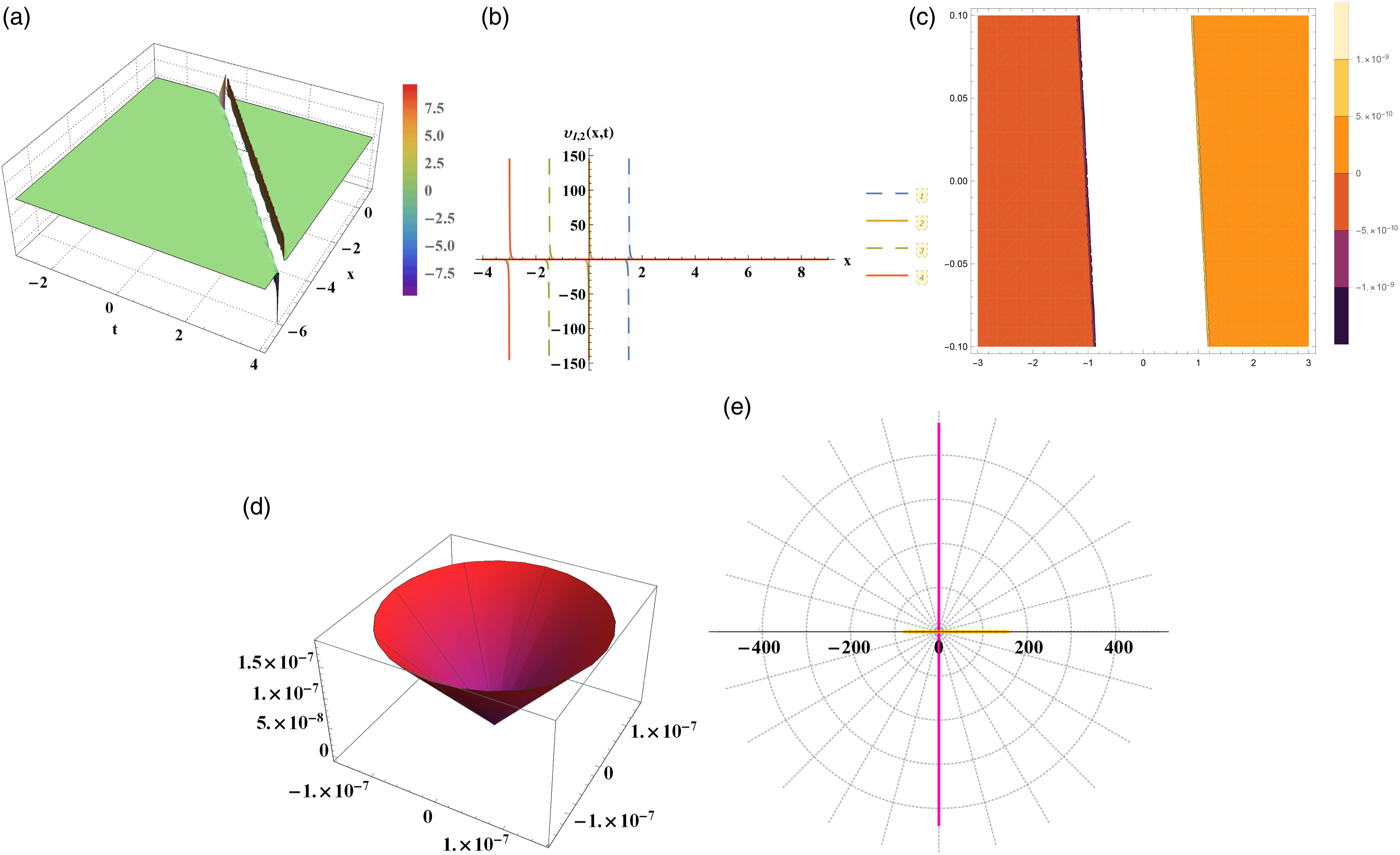
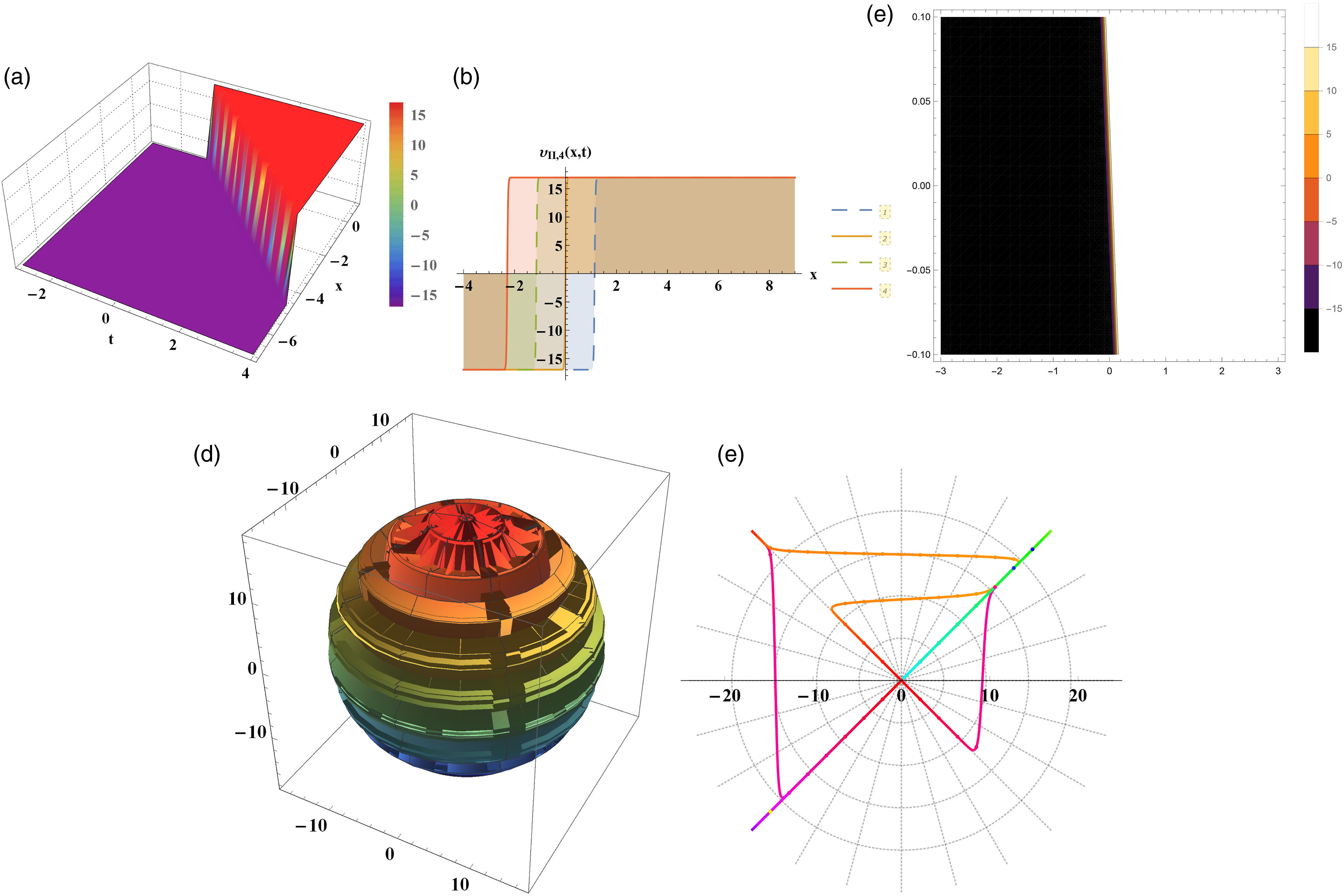
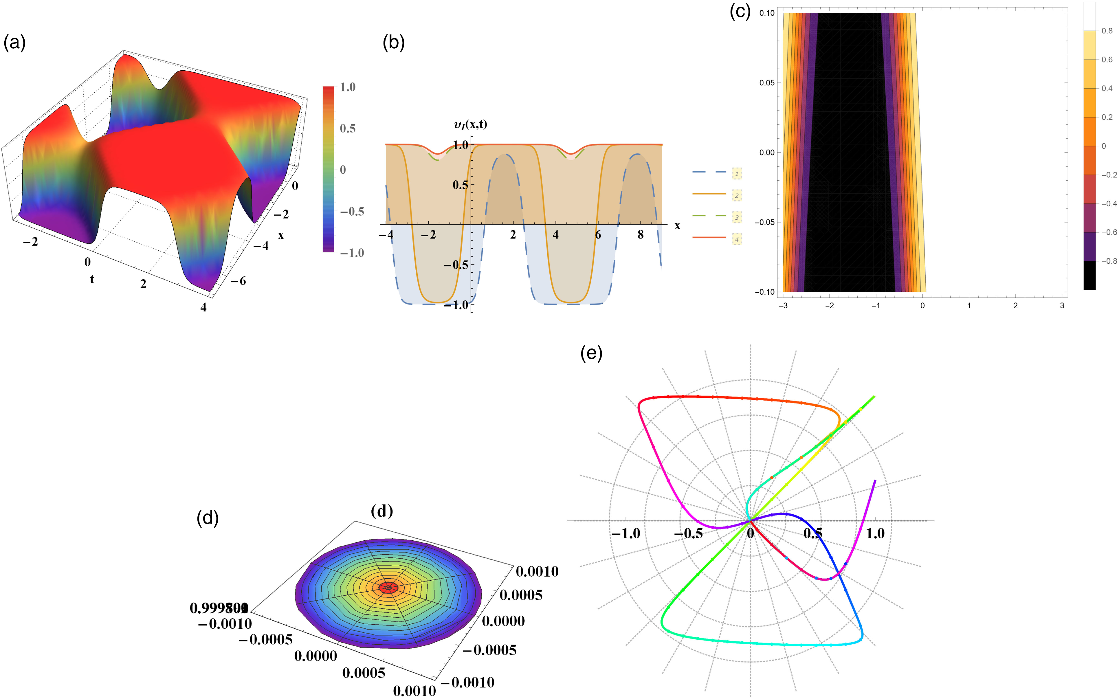
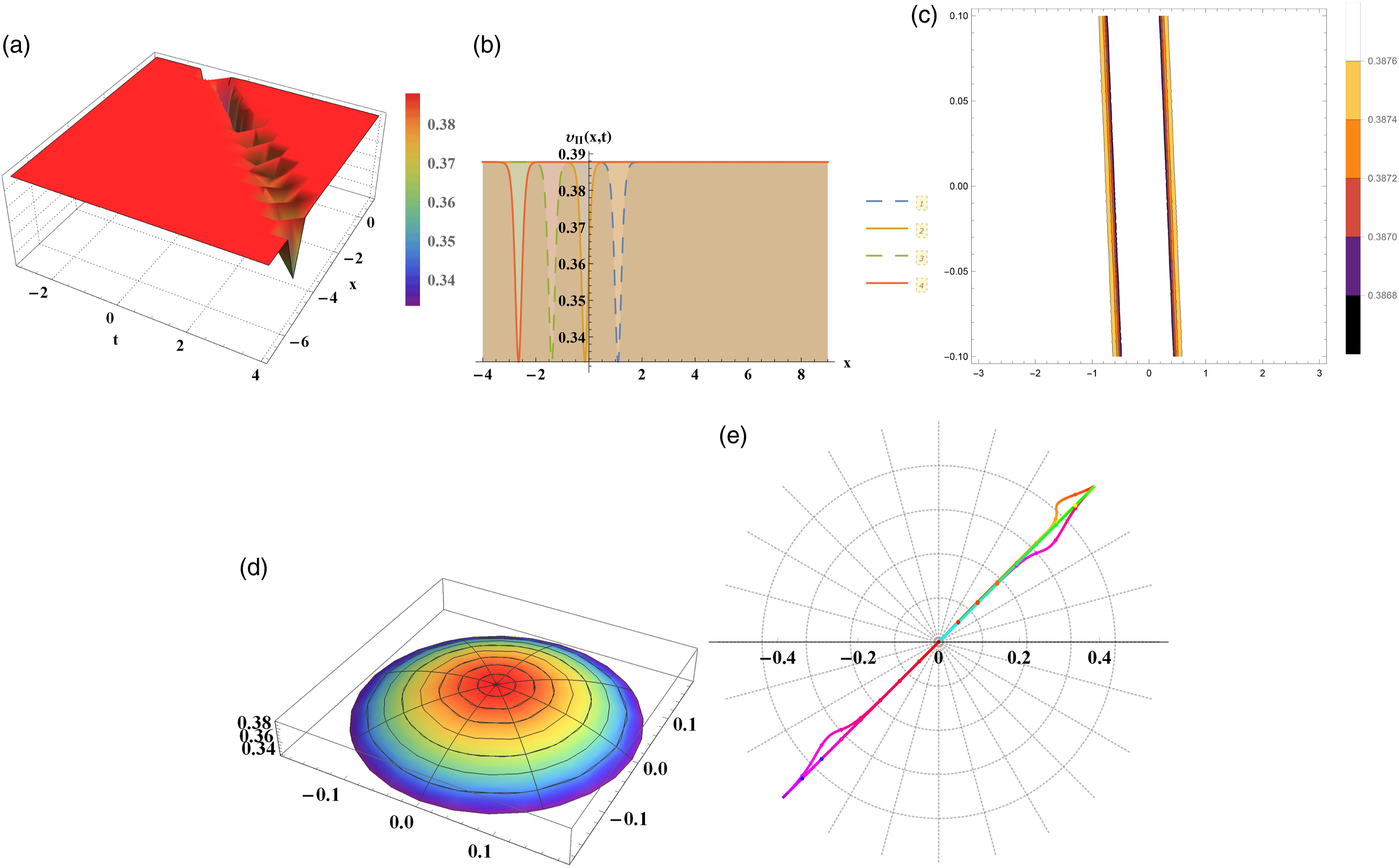
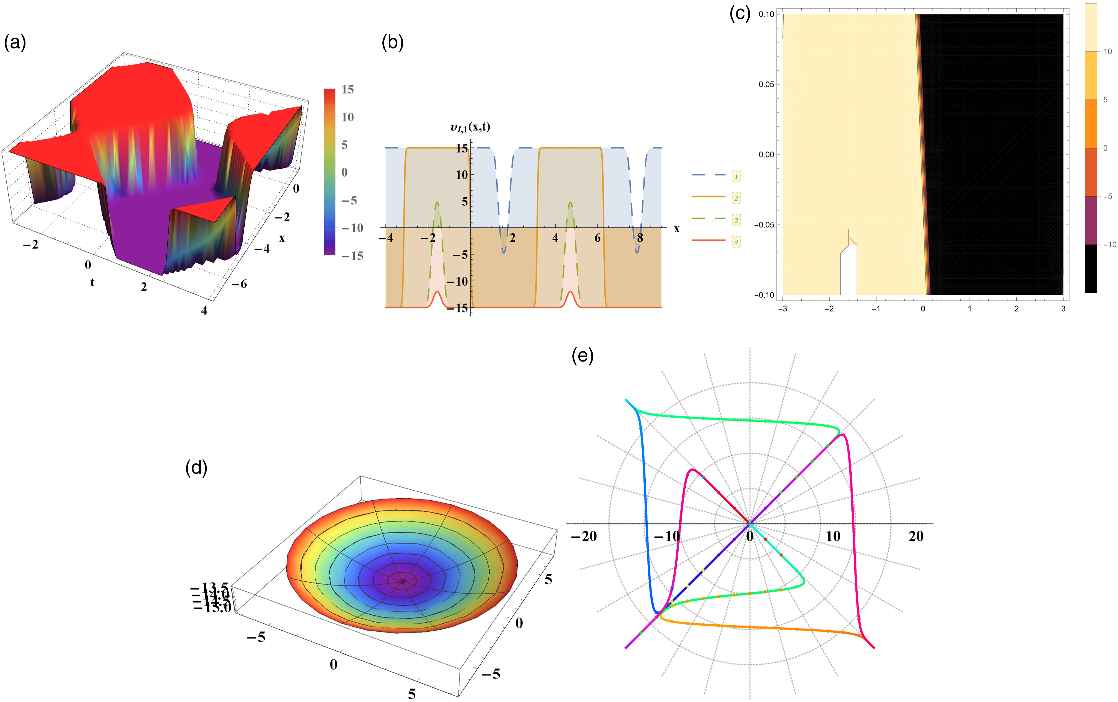
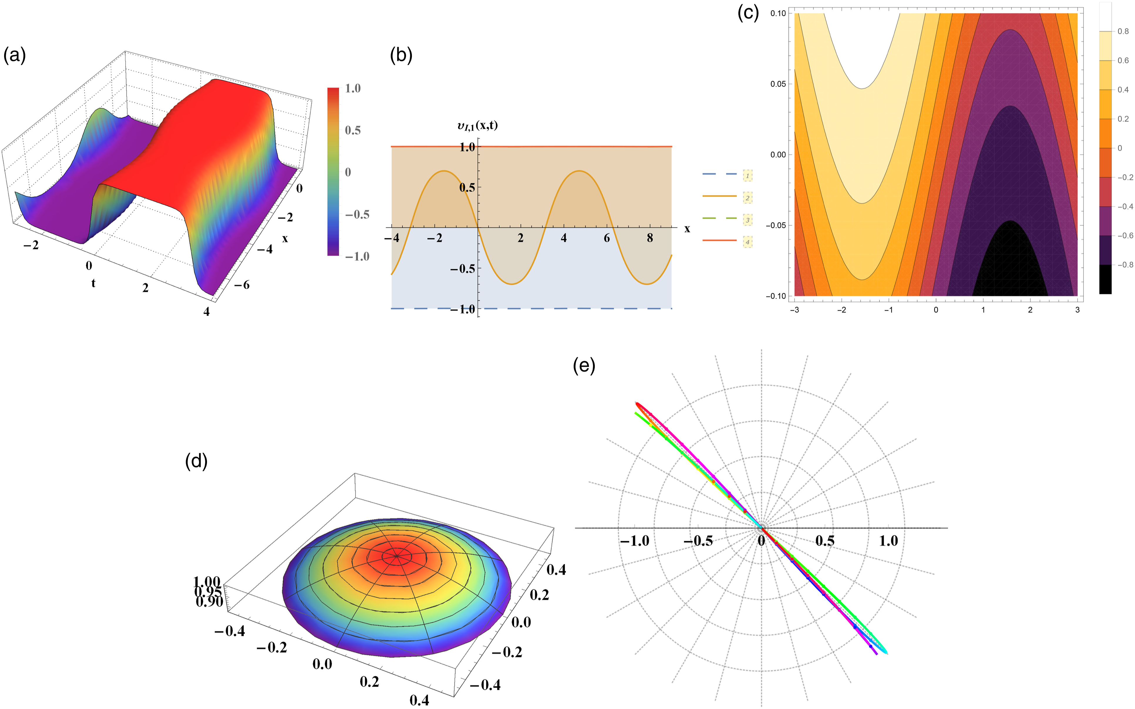
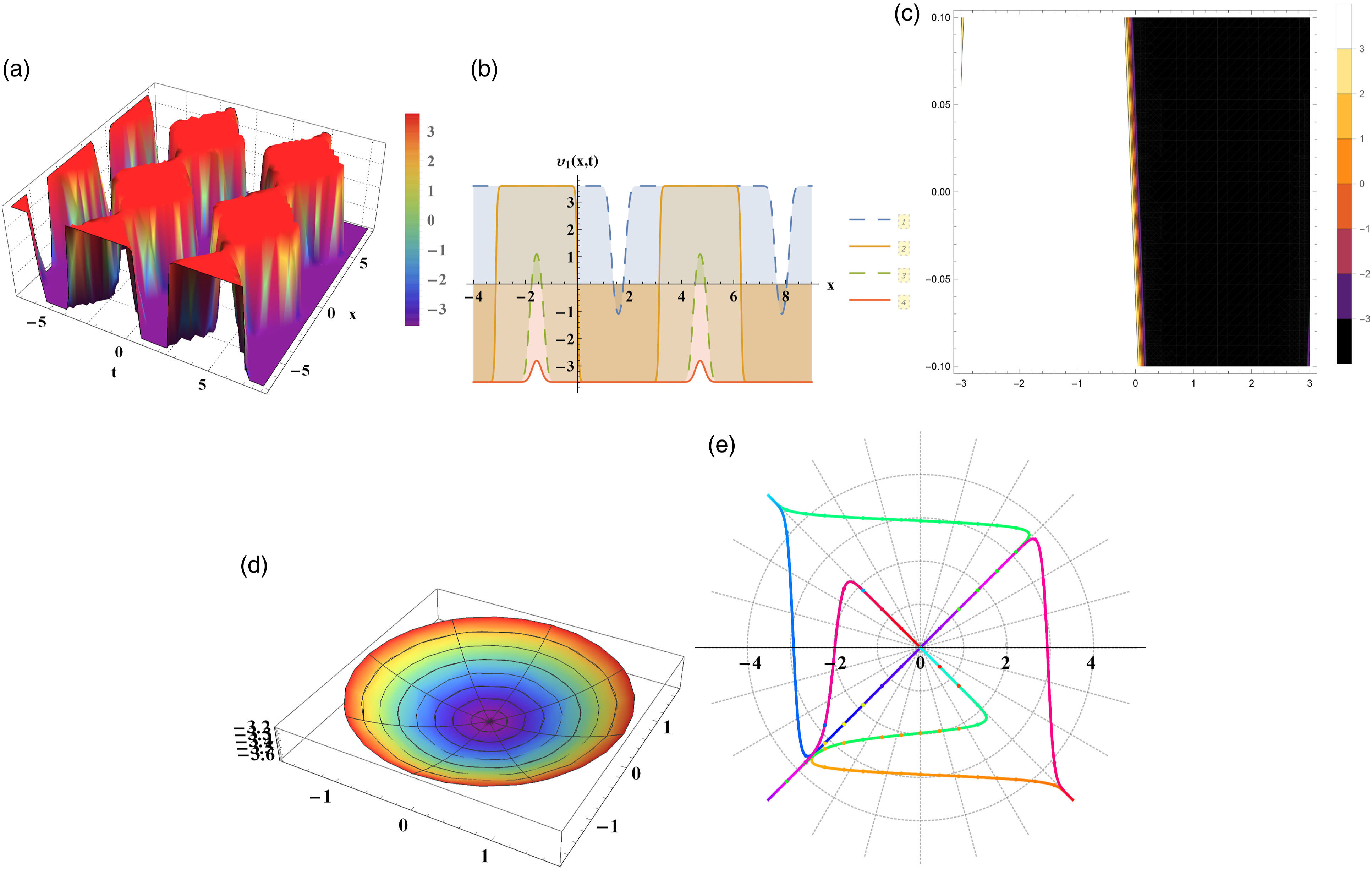
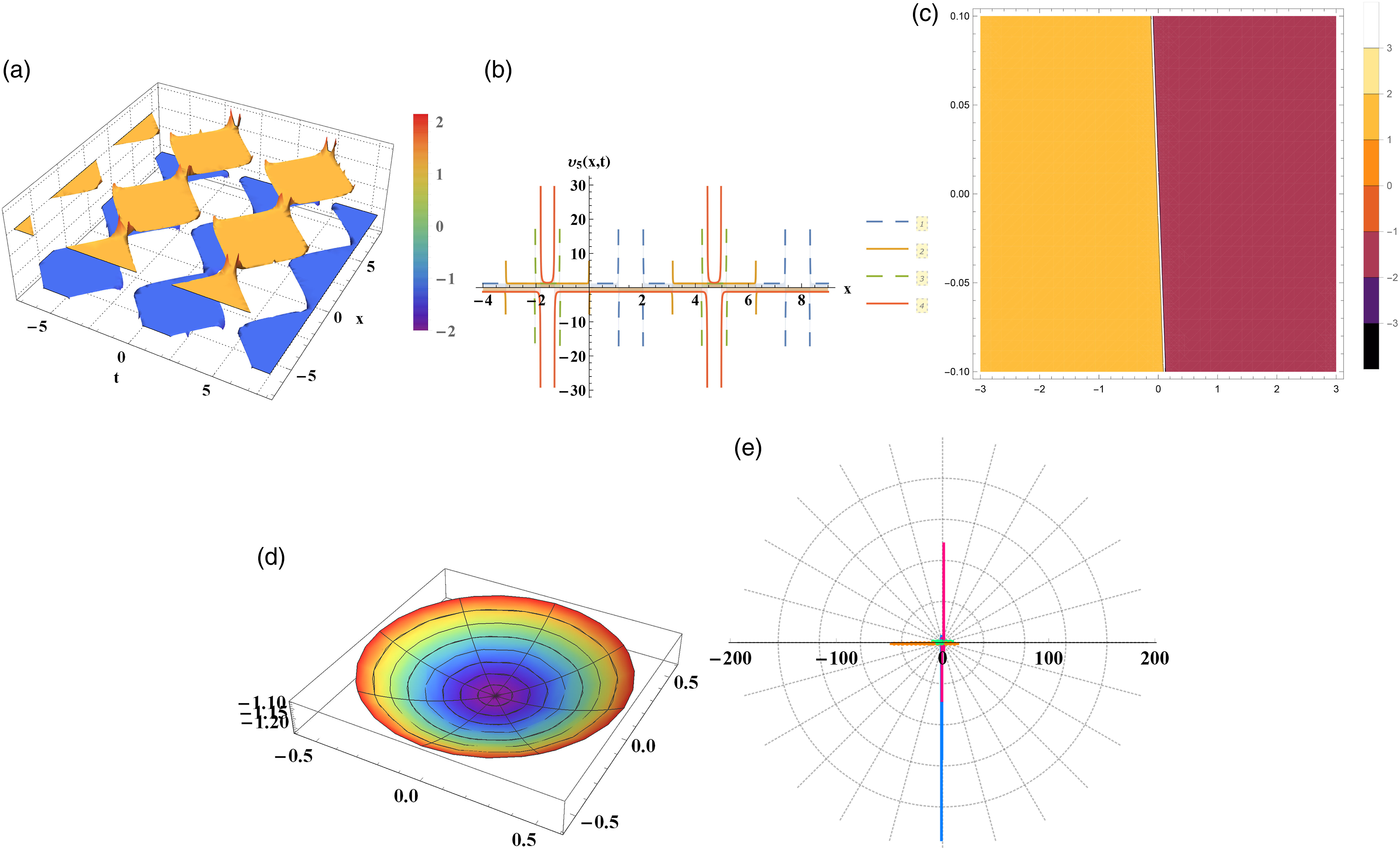
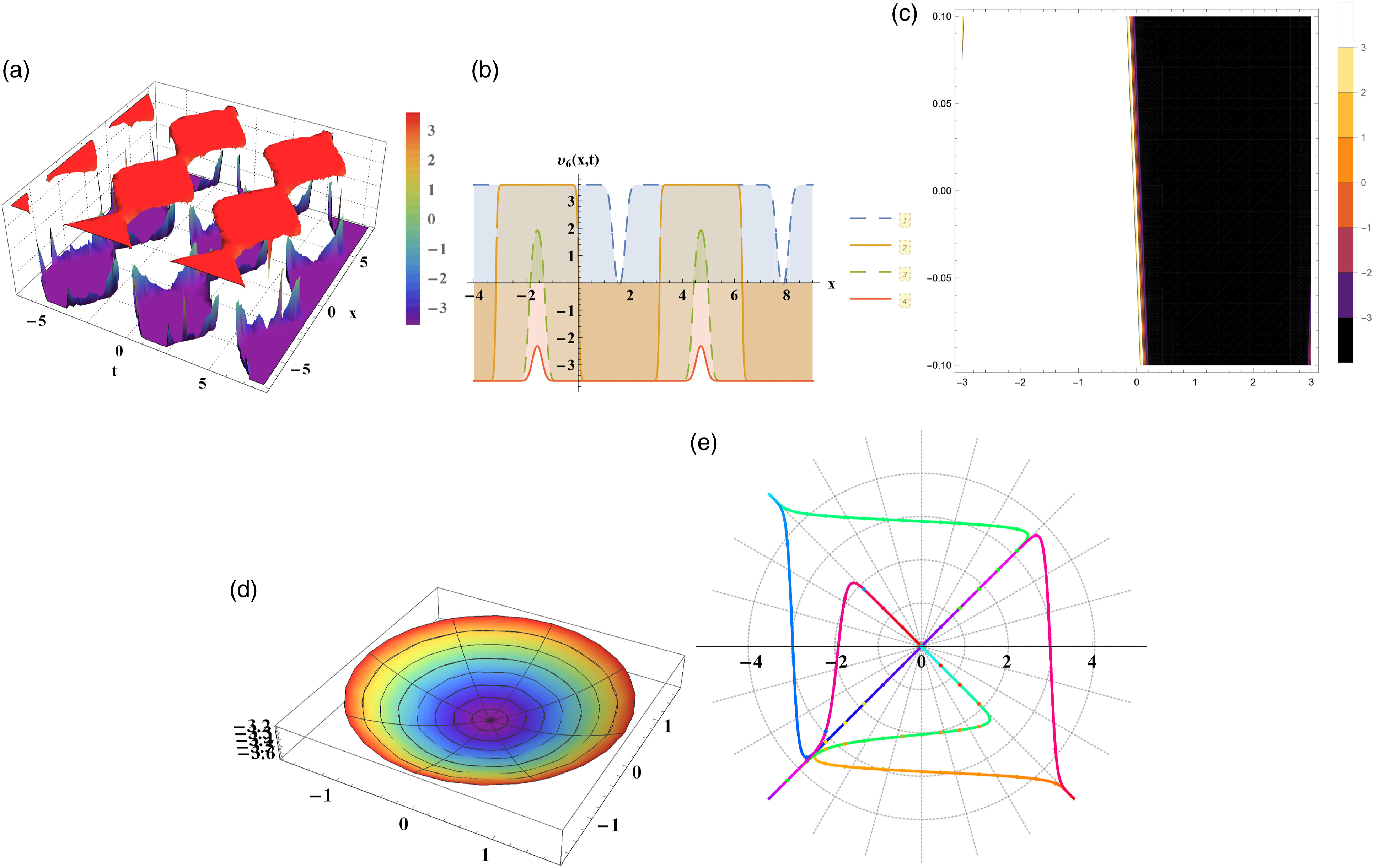
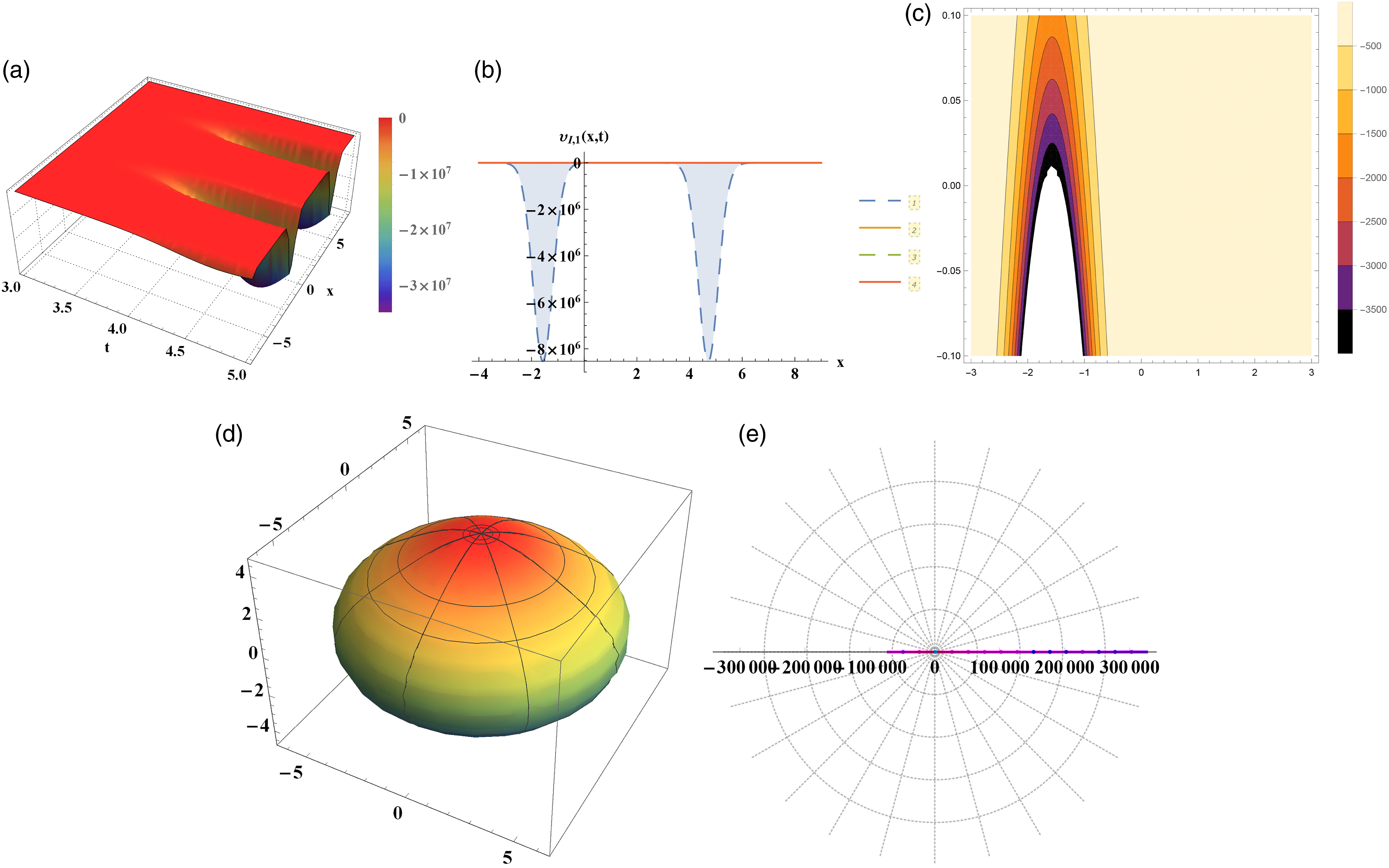
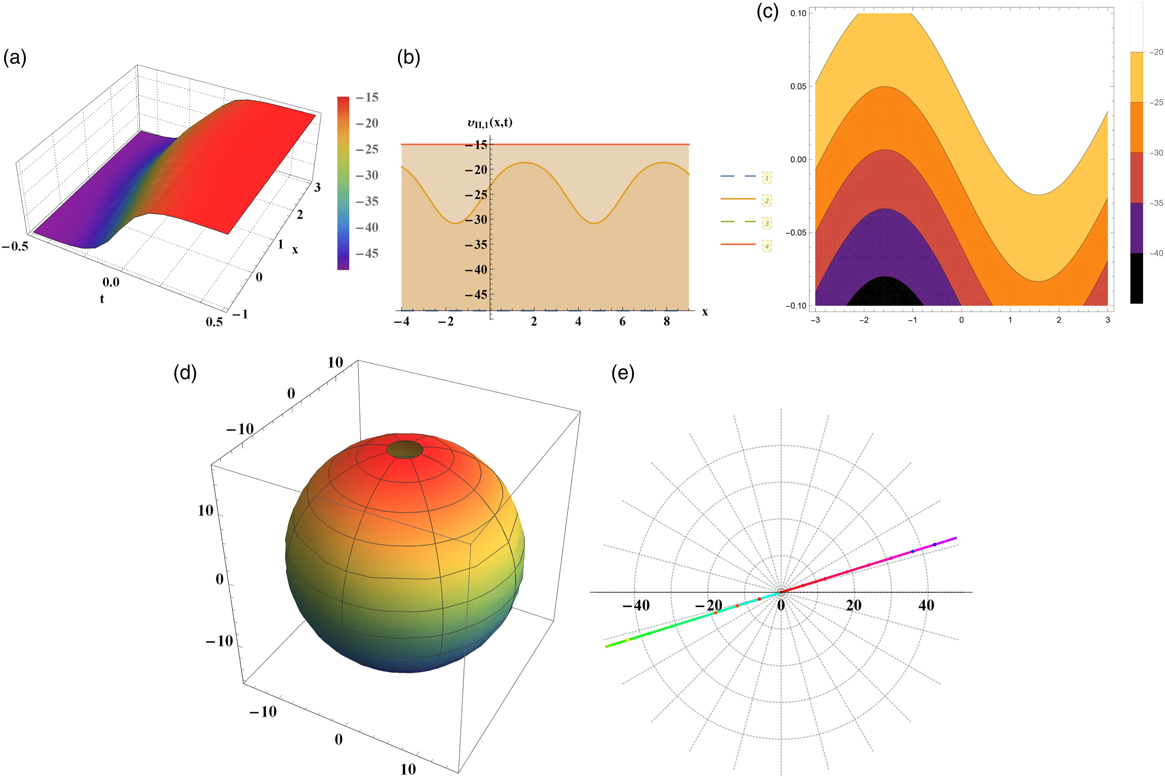
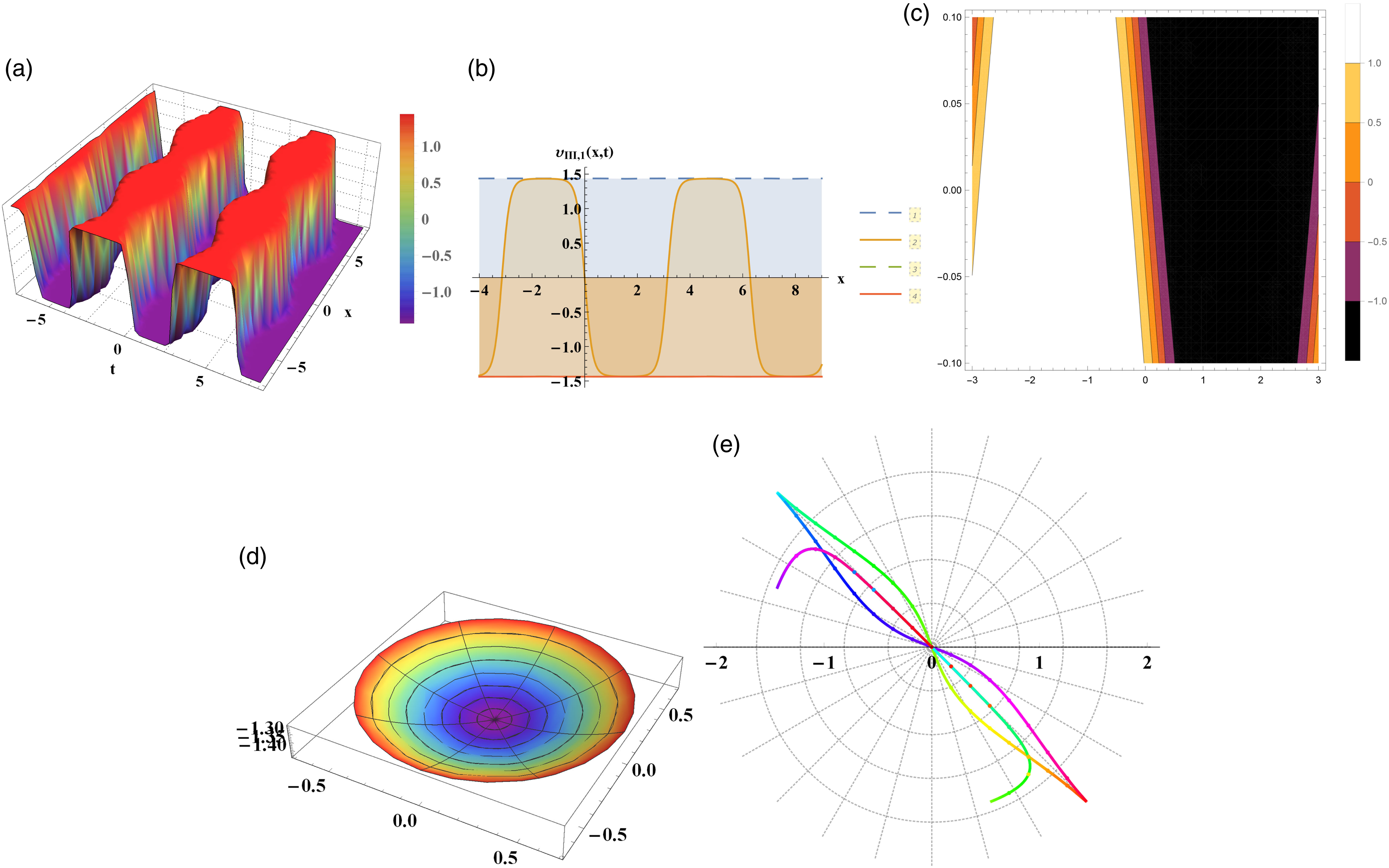
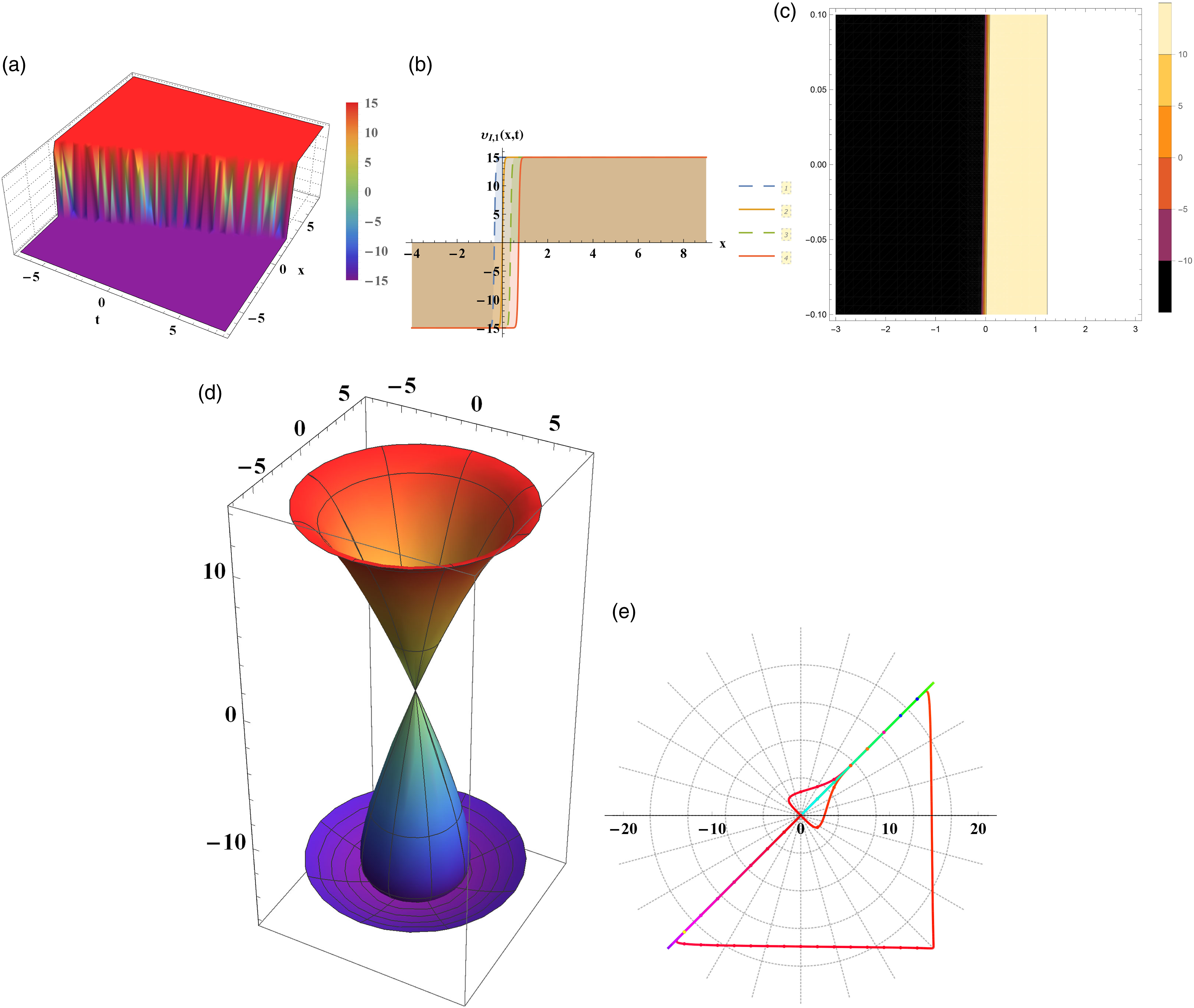
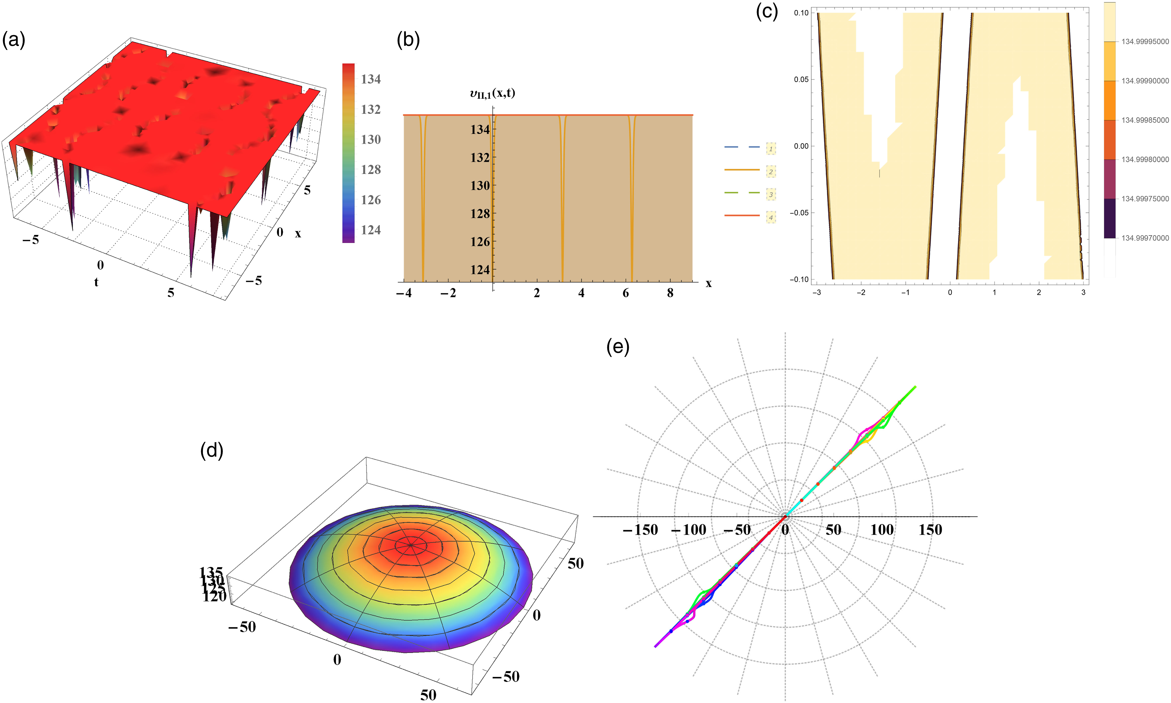
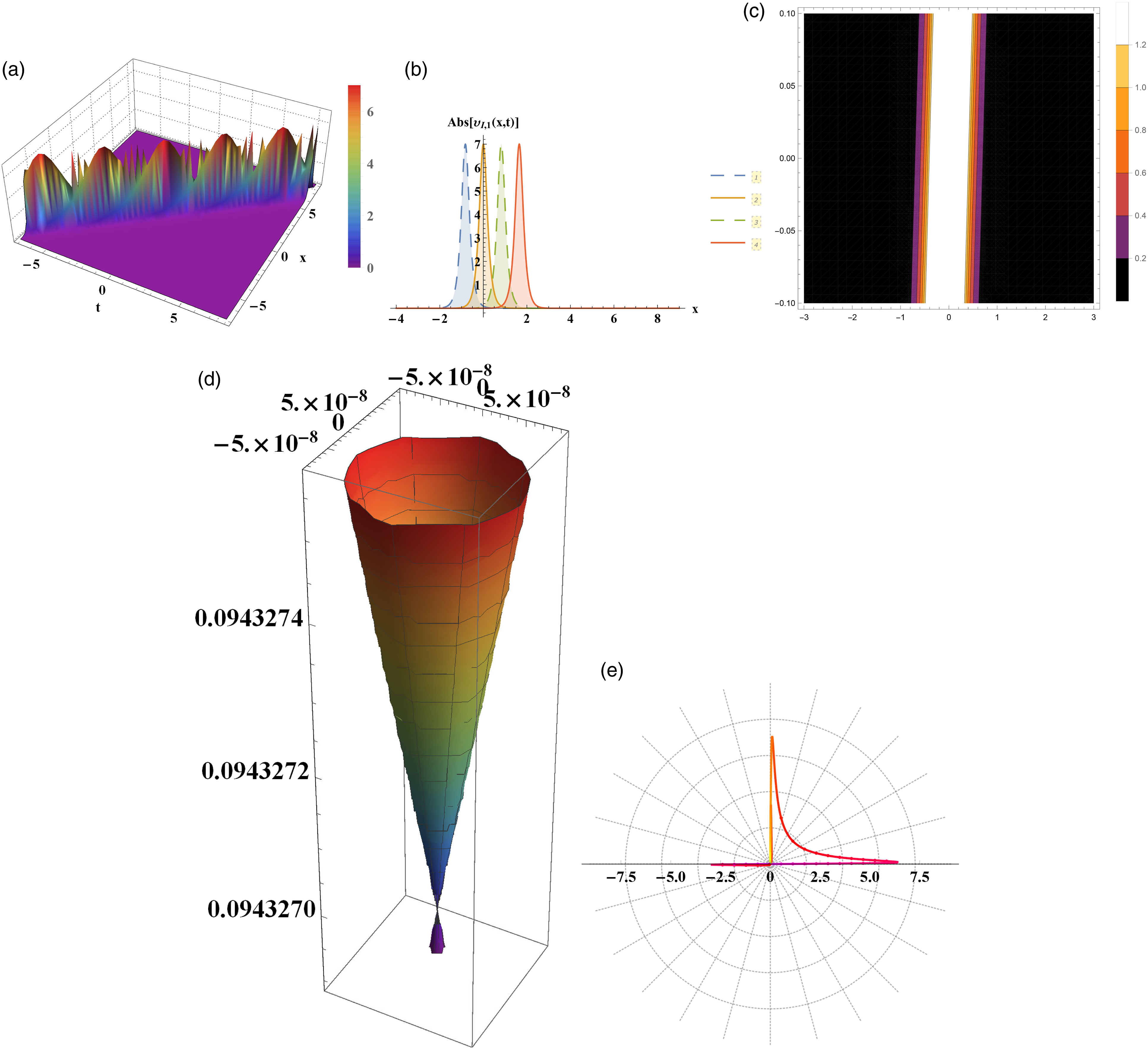
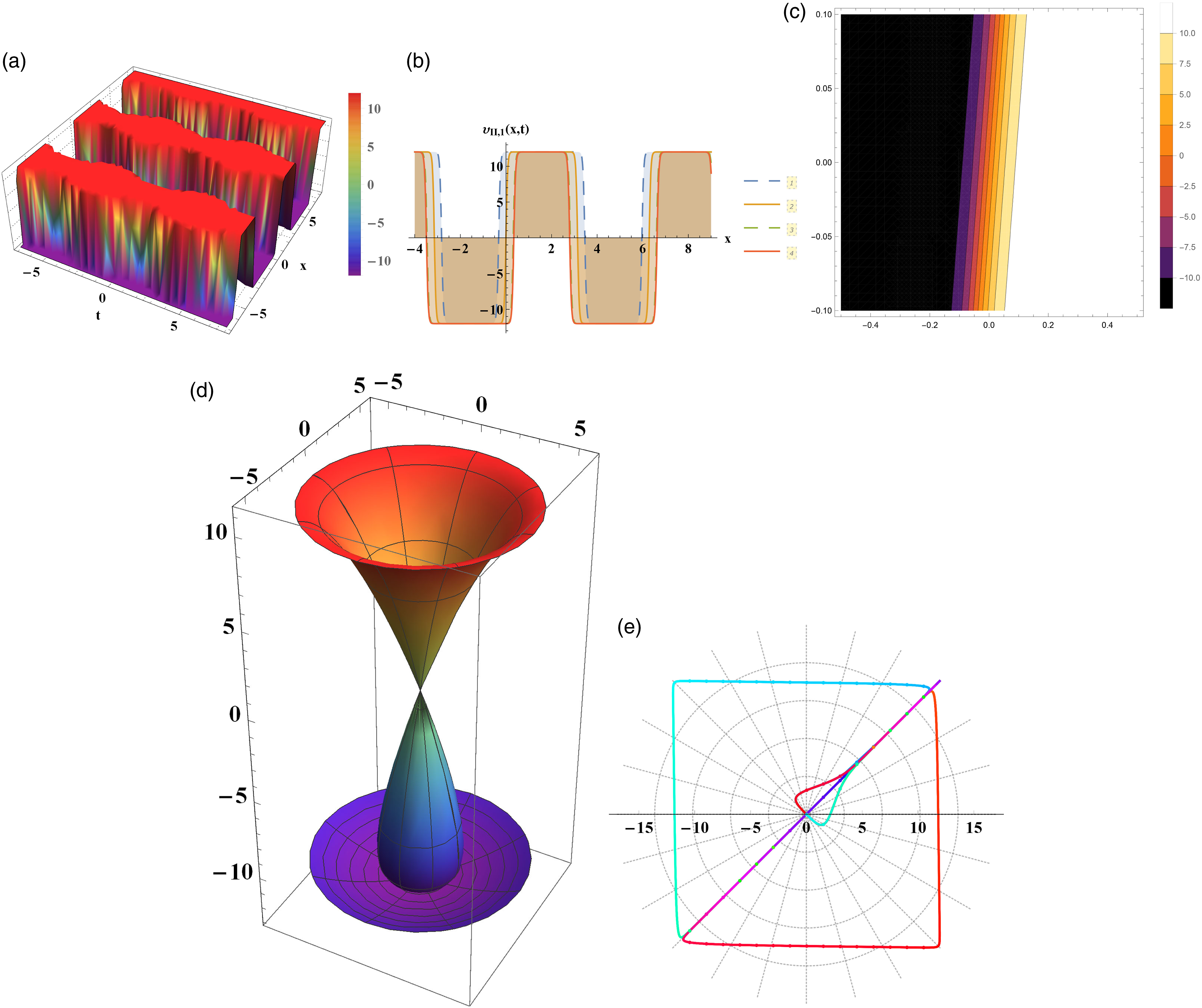
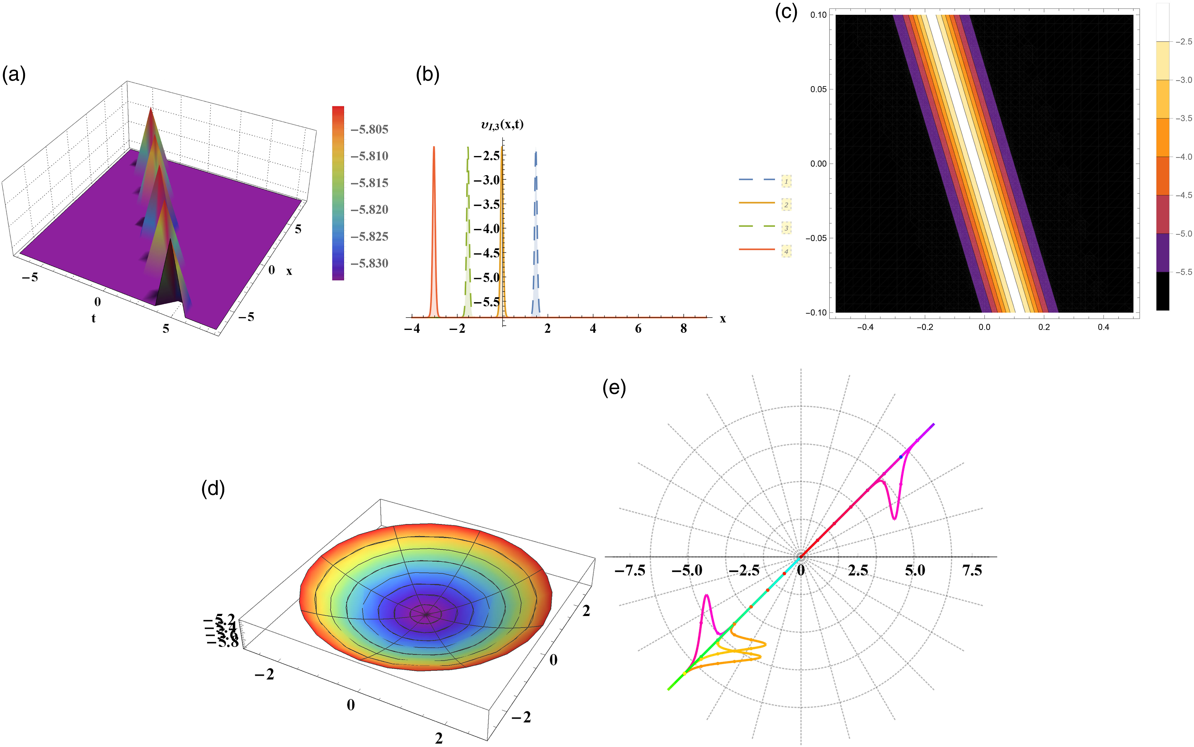
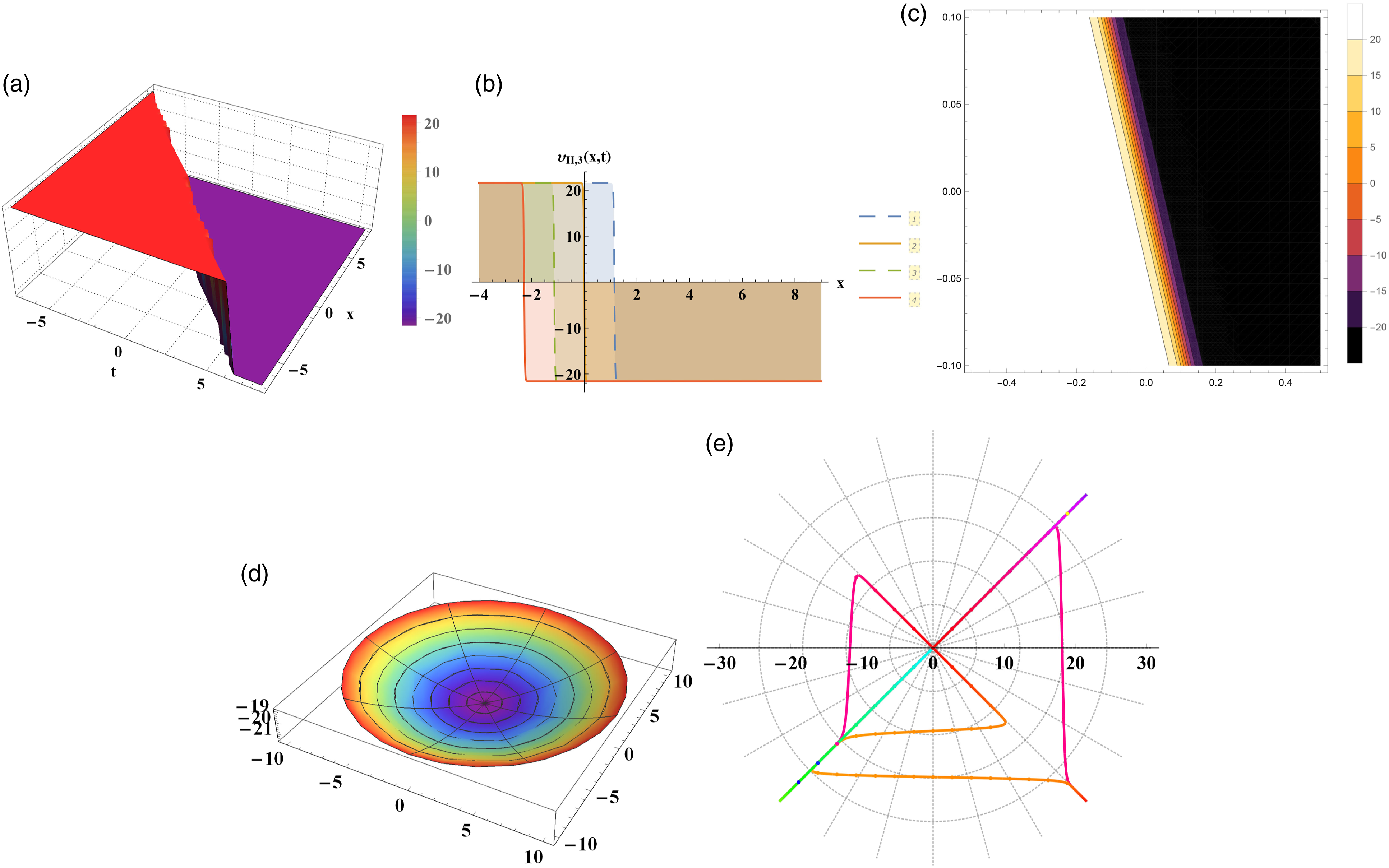
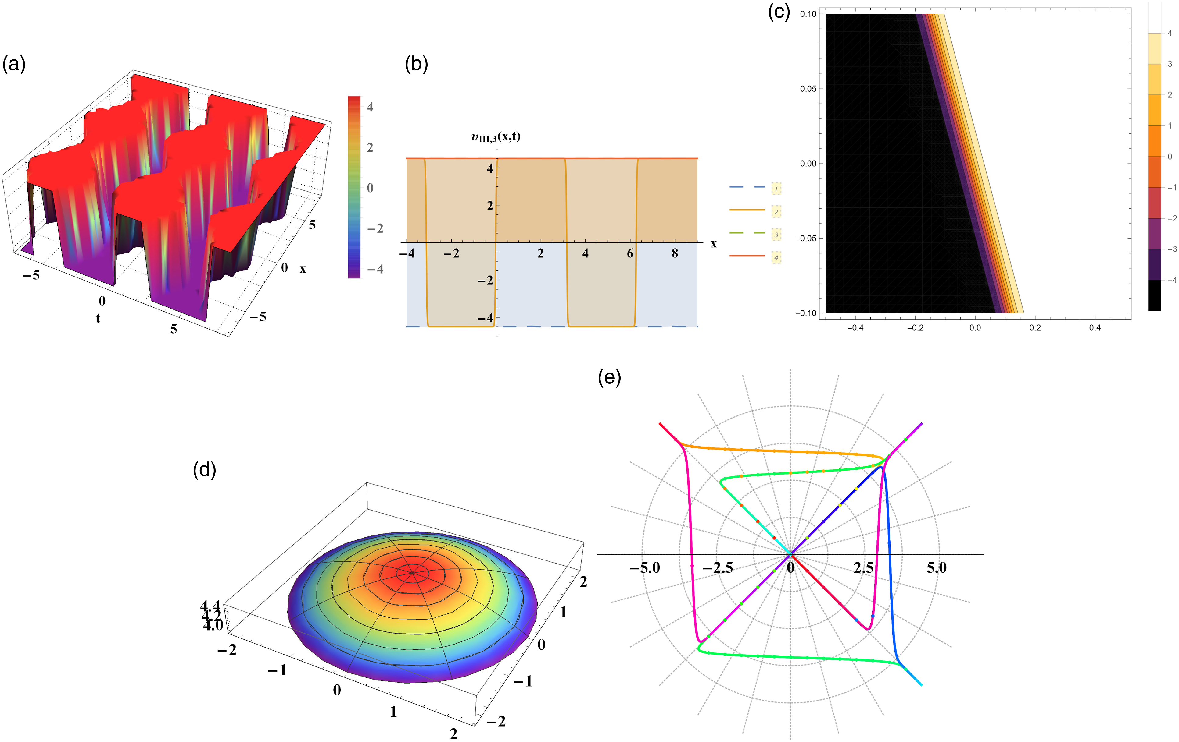
The merging MKdV with a negative MKdV equation was used in this paper to create unique explicit traveling wave solutions using eleven current approaches. Numerous special formulas for exponential, trigonometric, and hyperbolic solutions have been employed to represent the investigated model’s wave solutions. These solutions define the physical qualities more straightforwardly and across a considerably broader range, which enables us to apply our obtained responses in the models’ application. Now, and in this portion of our article, we will examine our solutions and their relationships and the techniques themselves to make the primary notion of these approaches evident. From an essential examination of our obtained answers, we can observe that a large number of ways provide solutions. These solutions have two parts; the first part is closed to other solutions that got by another manner, for example, [Equations (2.4), (2.6), (2.8), (2.26), (2.28), (2.34), (2.36), (2.47), (2.48), (2.50), (2.64), (2.67), (2.71), (2.72), (2.91), (2.103), (2.115), (2.172), (2.173), (2.187), (2.189), (2.205), (2.207), (2.210)], and so on. However, the second part is new formulas of solutions which are the rest of the solutions. These solutions have been represented in 3D, 2D, contour, spherical, and polar plots to show more physical and dynamical behavior of the investigated model ( Figures 1–24) by using some special values of the above shown parameters. Breather solitary wave of equation (2.4) in (a) 3D, (b) 2D, (c) contour, (d) spherical, and (d) polar plots. Kink solitary wave of equation (2.6) in (a) 3D, (b) 2D, (c) contour, (d) spherical, and (d) polar plots. Periodic solitary wave of equation (2.8) in (a) 3D, (b) 2D, (c) contour, (d) spherical, and (d) polar plots. Singular solitary wave of equation (2.26) in (a) 3D, (b) 2D, (c) contour, (d) spherical, and (d) polar plots. Periodic solitary wave of equation (2.28) in (a) 3D, (b) 2D, (c) contour, (d) spherical, and (d) polar plots. Singular solitary wave of equation (2.34) in (a) 3D, (b) 2D, (c) contour, (d) spherical, and (d) polar plots. Kink solitary wave of equation (2.36) in (a) 3D, (b) 2D, (c) contour, (d) spherical, and (d) polar plots. Kink solitary wave of equation (2.47) in (a) 3D, (b) 2D, (c) contour, (d) spherical, and (d) polar plots. Singular solitary wave of equation (2.48) in (a) 3D, (b) 2D, (c) contour, (d) spherical, and (d) polar plots. Solitary wave of equation (2.50) in (a) 3D, (b) 2D, (c) contour, (d) spherical, and (d) polar plots. Kink wave of equation (2.64) in (a) 3D, (b) 2D, (c) contour, (d) spherical, and (d) polar plots. Kink wave of equation (2.67) in (a) 3D, (b) 2D, (c) contour, (d) spherical, and (d) polar plots. Singular wave of equation (2.71) in (a) 3D, (b) 2D, (c) contour, (d) spherical, and (d) polar plots. Kink wave of equation (2.72) in (a) 3D, (b) 2D, (c) contour, (d) spherical, and (d) polar plots. Breather wave of equation (2.91) in (a) 3D, (b) 2D, (c) contour, (d) spherical, and (d) polar plots. Kink wave of equation (2.103) in (a) 3D, (b) 2D, (c) contour, (d) spherical, and (d) polar plots. Solitary wave of equation (2.115) in (a) 3D, (b) 2D, (c) contour, (d) spherical, and (d) polar plots. Kink wave of equation (2.172) in (a) 3D, (b) 2D, (c) contour, (d) spherical, and (d) polar plots. Cone solitary wave of equation (2.173) in (a) 3D, (b) 2D, (c) contour, (d) spherical, and (d) polar plots. Breather wave of equation (2.187) in (a) 3D, (b) 2D, (c) contour, (d) spherical, and (d) polar plots. Kink solitary wave of equation (2.189) in (a) 3D, (b) 2D, (c) contour, (d) spherical, and (d) polar plots. Breather solitary wave of equation (2.205) in (a) 3D, (b) 2D, (c) contour, (d) spherical, and (d) polar plots. Kink solitary wave of equation (2.207) in (a) 3D, (b) 2D, (c) contour, (d) spherical, and (d) polar plots. Periodic solitary wave of equation (2.210) in (a) 3D, (b) 2D, (c) contour, (d) spherical, and (d) polar plots.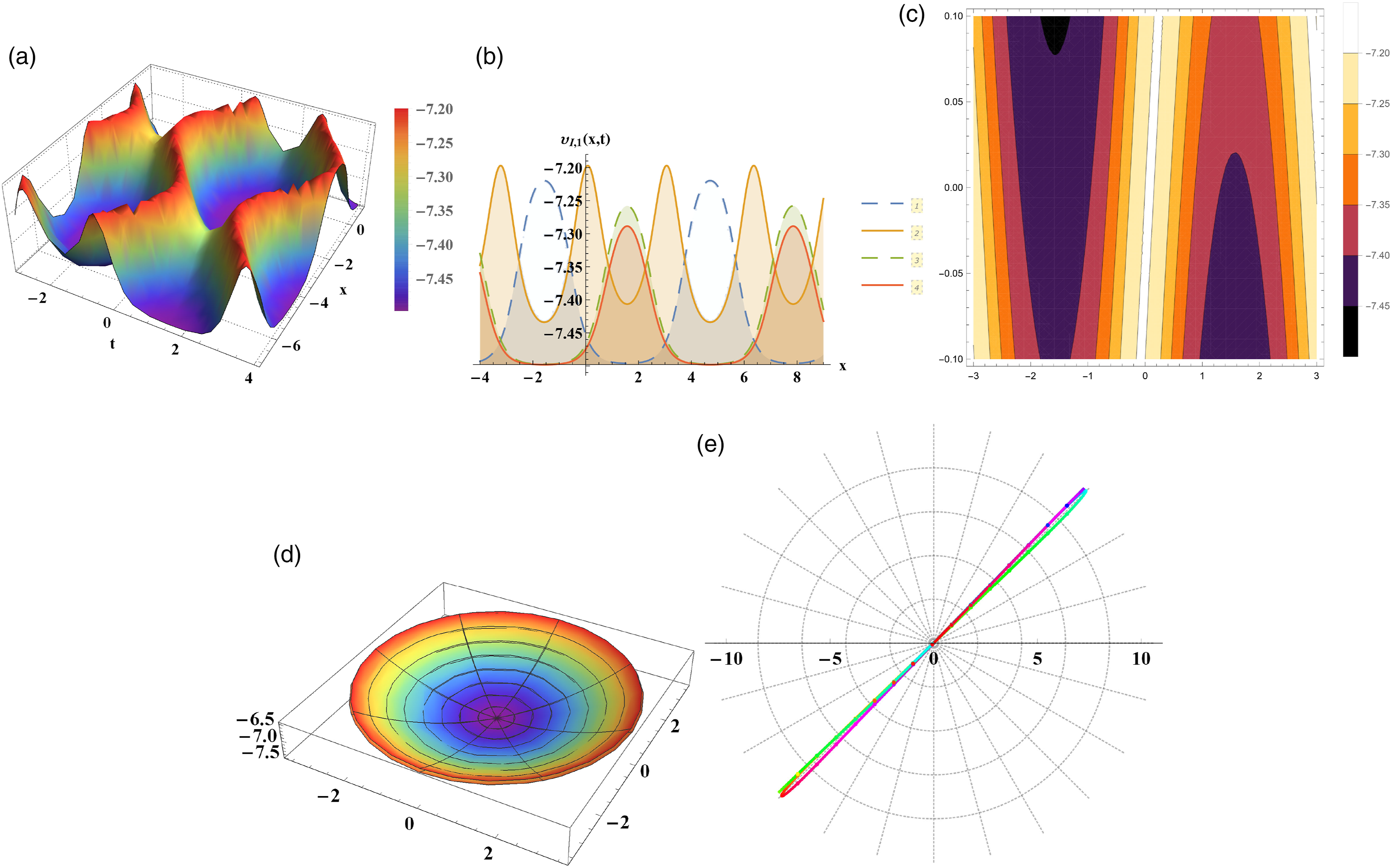
Convergence and divergence of solutions may be traced back to the similarity of techniques in the auxiliary equation, which is often a remarkable instance of the Riccati equation.
Conclusion
We utilized eleven techniques to the Merged MKdV with a negative MKdV equation in this research. We obtained several innovative formulas for this model’s sophisticated solitary wave solutions. Complex solitary wave solutions are used to explain the propagation of waves. Additionally, it is considered a more mathematically succinct tool for elaborating on the physical features of models. A representation of complicated solutions simplifies the handling of wave superpositions significantly. The correctness of all solutions found has been verified using the Mathematica software.
Footnotes
Acknowledgments
We greatly thank Taif University for providing fund for this work through Taif University Researchers Supporting Project number (TURSP-2020/52), Taif University, Taif, Saudi Arabia.
Authors’ contribution
Dexu Zhao and Mostafa Khater have revised the conceptualization, data curation, and methodology. Dianchen Lu and Mostafa Khater have revised data curation, investigation, and software. Samir Salama and Piyaphong Yongphe have revised the physical meaning of the obtained solutions and raised the given graphs resolutions. All authors have read and agreed to the published version of the manuscript.
Declaration of conflicting interests
The author(s) declared no potential conflicts of interest with respect to the research, authorship, and/or publication of this article.
Funding
The author(s) disclosed receipt of the following financial support for the research, authorship, and/or publication of this article: We greatly thank Taif University for providing fund for this work through Taif University Researchers Supporting Project number (TURSP-2020/52), Taif University, Taif, Saudi Arabia.
Availability of data and material
The data that support the findings of this study are available from the corresponding author upon reasonable request.
Code availability
The used code of this study is available from the corresponding author upon reasonable request.