Sage Journals: Discover world-class research

Abstract

The nonlinear partial differential equations considered in this study are important in modeling complex wave phenomena extending from hydrodynamics via ocean engineering to plasma physics, fluid dynamics, and other mediums. The Rosenau equation provides an analytical solution for studying wave phenomena in many physical systems, where dispersion and nonlinear dynamics play significant roles. This equation is proposed to explain the dense dynamic behavior of discrete systems. The generalized exponential rational function method has been employed to obtain the new soliton solutions of a nonlinear wave equation in fluid dynamics. This work uses the conformal fractional derivative and the fractional wave transformation to get the analytical results. The solutions include trigonometric, hyperbolic, and exponential functions with possible representations into three-dimensional graphics showing wave dynamics. The study focuses on the nonlinear Rosenau equation, revealing wave features including dark and bright solitons, and kinks and anti-kink waves. We are examining how parameters may have their impact on stability and interactions. This work enhances our knowledge of nonlinear wave systems and their practical applications in fluid dynamics and materials science.

Keywords

Rosenau equation solitary waves exact solutions the generalized exponential rational function method

Introduction

Nonlinear partial differential equations (NLPDEs) are applicable in various physical modeling scenarios. These equations are essential for understanding the physical implications of several important theories, motivating researchers to pursue their exact solutions. Numerous techniques and methodologies have been developed and employed to tackle these challenges. These include, but are not limited to, the following: the $G / G^{'}$ extended approach,¹ the positive quadratic function method,² the variational iteration method,³ Sardar subequation technique,⁴ the Adomian method,⁵ the Backlund technique,⁶ $\exp (- ϕ)$ -expansion method,⁷ the inverse scattering technique,⁸ new extended direct algebraic method,⁹ Kudryashov techniques,¹⁰ the auxiliary method,^11–14 the Hirota bilinear method,^15,16 and the generalized exponential rational function (GERF), as well as exponential rational function method¹⁷ and its generalized approach.¹⁸ The goal of this article is to use the GERF approach¹⁹ to obtain several precise solutions to the Rosenau problem. Ordinary and fractional partial differential equations (FPDEs) have received a lot of interest because of their many applications in physics, engineering, biology, and fluid mechanics.²⁰ Fractional ordinary differential equations (ODEs),²¹ FPDEs, and integral equations²² have received a lot of attention in the physical world. FPDEs are shown to be crucial for characterizing a wide range of nonlinear physical and natural systems. The current study focuses on the nonlinear Rosenau equation.²³

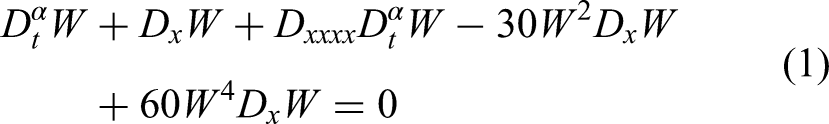
In this paper, we try to provide analytical solutions to the Rosenau problem. We consider the Rosenau equation²⁴ in the form

\begin{aligned} D_{t}^{α} W & + D_{x} W + D_{x x x x} D_{t}^{α} W - 30 W^{2} D_{x} W \\ + 60 W^{4} D_{x} W = 0 \end{aligned}

(1)

where

t

is the time and

x

is the spatial location in one dimension. Moreover,

α

is a free parameter, and the operator’s

D_{x}

and

D_{x x x}

are the typical integer-order differential operators in space. In contrast, the fractional derivative operators are denoted by

D_{t}^{α}

, where

α

is an integer between

0

and

1

Various numerical and analytical methods have been studied to investigate the dynamics of different Rosenau-type equations. Park²⁵ examined the solvability of the Rosenau equation and provided exact solutions. Atouani²⁶ employed a high-order conservative difference scheme to establish unconditional stability and convergence. Gao and Tian²⁷ applied the power series method to derive analytical solutions and further extended its use to obtain multiple exact results. Abbaszadeh and Dehghan²⁸ developed an element-free Galerkin approach based on two-grid interpolation for the nonlinear Rosenau regularized long-wave equation. For the Rosenau–Korteweg–de Vries–regularized long-wave (Rosenau–KdV–RLW) equation,²⁹ soliton and periodic solutions were obtained through the sine–cosine and tanh methods,³⁰ as well as via the mixed finite-element method.³¹ A collocation finite-element method based on quintic B-splines was also proposed for this problem,³² while Razborova et al.³³ studied shallow water waves using the Rosenau–KdV–RLW model. Ak et al.³⁴ used the subdomain technique with sextic B-spline basis functions to compute numerical solutions for the Rosenau–KdV problem. Erbay et al.³⁵ solved solitary wave solutions of the Rosenau equation using the Petviashvili iteration method, demonstrating robustness to initial guesses and rapid convergence. Guo et al.³⁶ proposed a multiple integral finite volume scheme for the Rosenau–KdV equation, showing it to be highly accurate, conservative, stable, and reliable. Chung and Pani³⁷ provided error estimates for the $C^{1}$ -finite-element method, while Omrani et al.³⁸ introduced a Galerkin–Crank–Nicolson fully discrete method and supplied error analysis for a semi-discrete finite-element approach to the Rosenau–Burgers problem. Alotaibi and Althobaiti³⁹ obtained exact traveling wave solutions, including exponential forms, for the Rosenau equation using the extended auxiliary equation method.

A number of studies have developed fractional calculus methods to obtain exact wave solutions of nonlinear equations. Shakeel et al.⁴⁰ employed the modified Riemann–Liouville derivative with wave transformation to transform the fractional modified Camassa-Holm equation into an ODE, in which the new $(G^{'} / G^{2})$ -expansion method provided soliton solutions. Mumtaz et al.⁴¹ also utilized a modified $(G^{'} / G^{2})$ -expansion method with $β$ , $M$ -truncated, and conformable derivatives to the (2 + 1)-dimensional nonlinear Wazwaz Kaur Boussinesq equation to derive soliton solutions and studied the dynamics through bifurcation and Poincaré maps. Shakeel⁴² generalized this with $β$ -derivatives for the $β$ -Peyrard–Bishop deoxyribonucleic acid model, while Shakeel et al.⁴³ also utilized conformable derivatives with the $(G^{'} / G^{2})$ -expansion method to three-dimensional Wazwaz–Benjamin–Bona Mahony equations, yielding hyperbolic and periodic solutions. Parallel developments highlight Jumarie and conformable derivatives in determining fractional traveling wave solutions. Almatrafi⁴⁴ used conformable derivatives with the enhanced extended tanh-function method to the fractional Fokas equation and achieved bell-shaped, kink, and anti-kink solitons. Alzubaidi and Almatrafi⁴⁵ used Jumarie’s derivative with unified and Kudryashov-type methods for the fractional symmetric regularized long wave (SRLW) equation and achieved solitary and periodic waves whose stability was verified via phase portraits. They also employed Jumarie’s derivative to derive solitary and periodic solutions of the fractional Boussinesq and SRLW equations through modified extended tanh, P-expansion, and $F^{'} / F$ -expansion techniques.^46–49 In other research, Berkal and Almatrafi⁵⁰ examined the conformable fractional Gierer–Meinhardt system, exhibiting equilibrium patterns and bifurcations. Lastly, Almatrafi et al.⁵¹ applied fractional derivatives in the generalized Riccati mapping technique to the Sharma–Tasso–Olver equation, resulting in trigonometric and rational solutions, and examining stability and chaos.

In this work, we propose the GERF method (GERFM) as an effective approach for solving the Rosenau equation. Our aim is to extend existing results by deriving new families of analytical solutions. Using GERFM, solutions are systematically classified into distinct cases and families, offering a wider variety of wave structures than previously reported. The GERFM approach is based on transforming a partial differential equation into an ODE through a suitable change of variables. This method has already been successfully applied to several nonlinear models, including the Ostrovsky equation, the $(1 + 1)$ -dimensional SRLW equation, and the fractional perturbed Radhakrishnan–Kundu–Lakshmanan model.^52,53 Jannat et al.⁵⁴ further demonstrated its effectiveness by obtaining accurate solutions for the $(2 + 1)$ -dimensional KdV equation. The motivation of the study comes from the necessity to better understand the nonlinear wave dynamics governed by the Rosenau equation that is encountered in fluid dynamics, plasma physics, and material science. The GERFM with conformable fractional derivatives presents an efficient approach. Using this framework makes it possible to find soliton solutions such as dark, bright, kink, and anti-kink. We also show how fractional parameters affect wave stability and interactions.

The subsequent sections of this paper present some definitions and properties of conformable derivatives, then the framework of GERFM for addressing the governing equation, followed by its application to the Rosenau problem. Finally, results and graphical illustrations are provided before drawing conclusions.

Preliminaries of conformable derivatives

One particular fractional derivative, the conformable derivative, maintains some of the properties of traditional derivatives but extends the notion of integer-order derivatives to the fractional case. Through an analysis of the idea of conformable derivatives and their main properties, this paper tries to present a new insight into this subject.

In this section, we discuss some basic conformable fractional-order derivatives. It allows us to have a better understanding of the result of physical behavior.

Definition 1

A function $h : [0, \infty) \to R$ of order $n$ for $0 < α < 1$ is a conformable fractional derivative if.⁵⁵

D_{α} (h (t)) = lim_{ϕ \to 0} \frac{h (t + ϕ t^{1 - α}) - h (t)}{ϕ} \forall t > 0

(2)

Theorem 1

Suppose that $Δ$ and $p$ are differentiable functions at a point $t > 0$ and $0 < α < 1$ , then^55,56

$D_{α} (c ⋆ Δ + d ⋆ p) = c ⋆ D_{α} (Δ) + d ⋆ D_{α} (p)$ , $\forall c, d .$

$D_{α} (t^{u}) = u ⋆ (t^{u - α})$ , $\forall u .$

$D_{α} (Δ . p) = p ⋆ D_{α} (Δ) + Δ ⋆ D_{α} (p) .$

$D_{α} (\frac{Δ}{p}) = \frac{p ⋆ D_{α} (Δ) - Δ ⋆ D_{α} (p)}{p^{2}}$ .

For any constant $k$ , $D_{α} (k) = 0.$

$D_{α} (Δ) (t) = t^{1 - α} ⋆ \frac{d h (t)}{d t}$ , if $h$ is a differentiable function.

These are just some of the properties of fractional derivatives with order $α$ for $0 < α < 1$ . For more information on these properties, see Shahzad et al.⁵⁶

The technique

Step (1): The steps in the GERF approach are provided below. Where $x$ and $t$ are two independent variables in the form of the Rosenau equation:

Q (W, D_{t}^{α} W, D_{x} W, D_{t}^{2 α} W, D_{x x} W, \dots) = 0

(3)

where

Q

is a function in

W (x, t)

, together with its highest order partial derivatives and nonlinear terms of

W (x, t)

Step (2): To obtain the exact solutions for equation (3), we use the traveling wave equation

W = w (ξ), where ξ = \frac{c t^{α}}{α} + n x

(4)

with constant

n, c \neq 0

. We convert equation (3) to nonlinear ODEs shown below using equation (4):

F (w, w^{'}, w^{″}, w^{‴}, \dots) = 0

(5)

where

F

is a function in

w (ξ)

with derivatives

w^{'} (ξ)

w^{″} (ξ)

w^{‴} (ξ)

, etc., is an integrable differential equation.

Step (3): While maintaining the integral constants at zero, we integrate $F$ in equation (5) as far as it is feasible in the setting of $ξ$ .

Step (4): We assume that the outcome of step (3) contains a solution of the following type:

w (ξ) = \sum_{j = 1}^{K} v_{j} P (ξ)^{j} + \sum_{i = 1}^{K} q_{j} P (ξ)^{- j} + v_{0}

(6)

where

v_{0}

v_{i}

, and

q_{i}

are the unknown constants,

j = (0, 1, 2, \dots, K)

and

K = 1

Step (5): In this stage, we calculate the required derivatives of equation (6) using Mathematica and substitute them into equation (5) to obtain systems of equations.

Step (6): We solve the systems of equations derived in stage (5) by using Mathematica to obtain sets of constant values, which we called families.

Step (7): The families obtained at step (6) are substituted into the different wave functions to gain our desired solutions for equation (1).

Application of the method

We generate exact solutions for the Rosenau problem using our necessary approach. Now, by integrating equation (4) into equation (1), we obtain the ODE as

c n^{4} w^{⁗} + c w + 12 n w^{5} - 10 n w^{3} + n w = 0

(7)

Using the homogenous balanced principle on equation (7), we obtain $K = 1$ and insert it into equation (6) to have

w (ξ) = \frac{q_{1}}{P} + P v_{1} + v_{0}

(8)

where

v_{0}

and

v_{1}

are constants, where the specific solitary wave solutions are determined by the (complex or real) values

V_{1}

V_{2}

V_{3}

V_{4}

and

L_{1}

L_{2}

L_{3}

L_{4}

P = \frac{V_{1} \exp (ξ L_{1}) + V_{2} \exp (ξ L_{2})}{V_{3} \exp (ξ L_{3}) + V_{4} \exp (ξ L_{4})}

(9)

Solution sets

Family 1 of the solutions of equation (1)

If we take $[V_{1}, V_{2}, V_{3}, V_{4}] = [- 1, - 1, 1, - 1]$ and $[L_{1}, L_{2}, L_{3}, L_{4}] = [1, - 1, 1, - 1]$ , then equation (9) becomes

P (ξ) = - \frac{\cosh (ξ)}{\sinh (ξ)}

(10)

Equation (8) is substituted into equation (7) using equation (10) to produce the set of equations. The following constant values can be found by solving this set of equations in Mathematica:

n = - \frac{1}{2} {(- \frac{1}{2})}^{3 / 4}, v_{1} = - \frac{1}{2 \sqrt{2}}, q_{1} = - \frac{1}{2 \sqrt{2}}, v_{0} = 0, c = - \frac{1}{2} {(- \frac{1}{2})}^{3 / 4}

These parameter values were obtained using the outlined technique in section 3 of the GERFM with the substitutions of the ansatz functions into the reduced ODE, expanding, and collecting terms. This produced an algebraic system, which was then solved using Mathematica to determine the constants.

Suppose that $β = (- 1 / 2)^{3 / 4}$ , then

w_{1} (x, t) = - \frac{\tanh ((β t^{α} / 2 α) + (β x / 2))}{2 \sqrt{2}} - \frac{\coth ((β t^{α} / 2 α) + (β x / 2))}{2 \sqrt{2}}

(11)

Family 2 of the solutions of equation (1)

If we use $[V_{1}, V_{2}, V_{3}, V_{4}] = [- i, i, 1, 1]$ and $[L_{1}, L_{2},$ $L_{3}, L_{4}] = [i, - i, i, - i]$ , then equation (9) becomes,

P (ξ) = - \frac{\sin (ξ)}{\cos (ξ)}

(12)

The set of equations could be obtained by using equation (12) and substituting equation (8) in equation (7). This set of equations may be solved in Mathematica to find the following constant values:

v_{0} = 0, c = \frac{i}{4}, n = - \frac{i}{2}, v_{1} = \frac{1}{2}, q_{1} = \frac{1}{2}

Hence, our solution becomes

w_{2} (x, t) = \frac{1}{2} i \tanh (\frac{x}{2} - \frac{t^{α}}{4 α}) - \frac{1}{2} i \coth (\frac{x}{2} - \frac{t^{α}}{4 α})

(13)

Family 3 of the solutions of equation (1)

Taking $[V_{1}, V_{2}, V_{3}, V_{4}] = [1, 0, 1, 1]$ and $[L_{1}, L_{2}, L_{3},$ $L_{4}] = [1, 0, 1, - 0]$ , then equation (9) becomes

P (ξ) = \frac{\exp (ξ)}{\exp (ξ) + 1}

(14)

The set of equations may be obtained by using equation (14) and substituting equation (8) into equation (7). This set of equations may be solved in Mathematica to find the following constant values:

v_{0} = - \frac{1}{\sqrt{2}}, q_{1} = 0, v_{1} = \sqrt{2}, c = - \sqrt[4]{- 2}, n = - \sqrt[4]{- 2}

We suppose that $δ = - (- 1 / 2)^{3 / 4}$ , then

w_{3} (x, t) = \frac{\sqrt{2} e^{(δ t^{α} / α) + δ x}}{e^{(δ t^{α} / α) + δ x} + 1} - \frac{1}{\sqrt{2}}

(15)

Family 4 of the solutions of equation (1)

Using $[V_{1}, V_{2}, V_{3}, V_{4}] = [1 - i, 1 + i, 1, 1]$ and $[L_{1}, L_{2},$ $L_{3}, L_{4}] = [i, - i, i, - i]$ then, equation (9) becomes

P (ξ) = \frac{\sin (ξ) + \cos (ξ)}{\cos (ξ)}

(16)

The set of equations may be obtained by substituting equation (8) into equation (7) using equation (16). This set of equations may be solved in Mathematica to find the following constant values:

v_{0} = \frac{i}{\sqrt{2}}, c = {(- \frac{1}{2})}^{3 / 4}, n = {(- \frac{1}{2})}^{3 / 4}, v_{1} = - \frac{i}{\sqrt{2}}, q_{1} = 0

We suppose that $β = (- 1 / 2)^{3 / 4}$ , then

w_{4} (x, t) = \frac{i}{\sqrt{2}} - \frac{i \sec ((β t^{α} / α) + β x) (\sin ((β t^{α} / α) + β x) + \cos ((β t^{α} / α) + β x))}{\sqrt{2}}

(17)

Family 5 of the solutions of equation (1)

If we employ $[V_{1}, V_{2}, V_{3}, V_{4}] = [- 3, - 1, 1, 1]$ and $[L_{1}, L_{2}, L_{3}, L_{4}] = [1, - 1, 1, - 1]$ , then equation (9) becomes

P (ξ) = \frac{- \sinh (ξ) - 2 \cosh (ξ)}{\cosh (ξ)}

(18)

The set of equations may be obtained by utilizing equation (18) and replacing equation (8) into equation (7). This set of equations may be solved in Mathematica to find the following constant values:

v_{0} = - \sqrt{2}, c = {(- \frac{1}{2})}^{3 / 4}, n = {(- \frac{1}{2})}^{3 / 4}, v_{1} = - \frac{1}{\sqrt{2}}, q_{1} = 0

We suppose that $β = (- 1 / 2)^{3 / 4}$ , then

\begin{aligned} w_{5} (x, t) = - \frac{1}{\sqrt{2}} (sech (\frac{β t^{α}}{α} + β x) (- \sinh (β x + \frac{β t^{α}}{α}) \\ - 2 \cosh (\frac{β t^{α}}{α} + x β))) - \sqrt{2} \end{aligned}

(19)

Family 6 of the solutions of equation (1)

If we apply $[V_{1}, V_{2}, V_{3}, V_{4}] = [- 1, 0, 1, 1]$ and $[L_{1}, L_{2}, L_{3}, L_{4}] = [0, 1, 0, 1]$ , then equation (9) becomes

P (ξ) = - \frac{1}{\exp (ξ) + 1}

(20)

The set of equations may be obtained by substituting equation (8) into equation (7) utilizing equation (20). This set of equations may be solved in Mathematica to find the following constant values:

v_{0} = \frac{1}{\sqrt{2}}, c = \sqrt[4]{- 2}, n = \sqrt[4]{- 2}, v_{1} = \sqrt{2}, q_{1} = 0

We suppose that $γ = \sqrt[4]{- 2}$ , then

w_{6} (x, t) = \frac{1}{\sqrt{2}} - \frac{\sqrt{2}}{e^{(γ t^{α} / α) + γ x} + 1}

(21)

Family 7 of the solutions of equation (1)

Applying $[V_{1}, V_{2}, V_{3}, V_{4}] = [1, 0, 1, 1]$ and $[L_{1}, L_{2}, L_{3}, L_{4}] = [1, 0, 1, 0]$ then, equation (9) becomes

P (ξ) = - \frac{\sinh (ξ)}{\cosh (ξ)}

(22)

The set of equations may be obtained by using equation (22) and substituting equation (8) into equation (7). This set of equations may be solved in Mathematica to find the following constant values:

v_{0} = - \frac{1}{\sqrt{2}}, c = \sqrt[4]{- 2}, n = \sqrt[4]{- 2}, v_{1} = \sqrt{2}, q_{1} = 0

We suppose that $γ = \sqrt[4]{- 2}$ , then

w_{7} (x, t) = - \sqrt{2} \tanh (\frac{γ t^{α}}{α} + γ x) - \frac{1}{\sqrt{2}}

(23)

Family 8 of the solutions of equation (1)

If we adopt $[V_{1}, V_{2}, V_{3}, V_{4}] = [1 - i, - 1 - i, 1, 1]$ and $[L_{1}, L_{2}, L_{3}, L_{4}] = [i, 0, i, 0]$ , then equation (9) becomes

P (ξ) = \frac{\sin (ξ) + 2 \cos (ξ)}{\cos (ξ)}

(24)

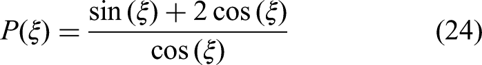
The set of equations may be obtained by substituting equation (8) into equation (7) using equation (24). This set of equations may be solved in Mathematica to find the following constant values:

v_{0} = - \frac{i}{\sqrt{2}}, c = - \sqrt[4]{- 2}, n = - \sqrt[4]{- 2}, v_{1} = - \frac{1}{\sqrt{2}}, q_{1} = 0

We suppose that $γ = \sqrt[4]{- 2}$ , then

w_{8} (x, t) = - \frac{\sec ((γ t^{α} / α) + γ x) (2 \cos ((γ t^{α} / α) + γ x) - \sin ((γ t^{α} / α) + γ x))}{\sqrt{2}} - \frac{i}{\sqrt{2}}

(25)

Family 9 of the solutions of equation (1)

If we operate $[V_{1}, V_{2}, V_{3}, V_{4}] = [1, 2, 1, 1]$ and $[L_{1}, L_{2}, L_{3}, L_{4}] = [1, 0, 1, 0]$ , then equation (9) becomes

P (ξ) = \frac{\exp (ξ) + 2}{\exp (ξ) + 1}

(26)

The set of equations may be obtained by using equation (26) and substituting equation (8) into equation (7). This set of equations may be solved in Mathematica to find the following constant values:

v_{0} = \frac{3}{\sqrt{2}}, c = \sqrt[4]{- 2}, n = \sqrt[4]{- 2}, v_{1} = - \sqrt{2}, q_{1} = 0

We suppose that $γ = \sqrt[4]{- 2}$ , then

w_{9} (x, t) = \frac{3}{\sqrt{2}} - \frac{\sqrt{2} (e^{(γ t^{α} / α) + γ x} + 2)}{e^{(γ t^{α} / α) + γ x} + 1}

(27)

Family 10 of the solutions of equation (1)

If we select $[V_{1}, V_{2}, V_{3}, V_{4}] = [2, 1, 1, 1]$ and $[L_{1}, L_{2}, L_{3}, L_{4}] = [1, 0, 1, 0]$ , then equation (9) becomes

P (ξ) = \frac{\exp (ξ)}{\exp (ξ) + 1}

(28)

The set of equations may be obtained by substituting equation (8) into equation (7) using equation (28). This set of equations may be solved in Mathematica to find the following constant values:

v_{0} = - \frac{3}{\sqrt{2}}, c = \sqrt[4]{- 2}, n = \sqrt[4]{- 2}, v_{1} = \sqrt{2}, q_{1} = 0

We suppose that $γ = \sqrt[4]{- 2}$ , then

w_{10} (x, t) = \frac{\sqrt{2} e^{(γ t^{α} / α) + γ x}}{e^{(γ t^{α} / α) + γ x} + 1} - \frac{3}{\sqrt{2}}

(29)

Family 11 of the solutions of equation (1)

If we consider $[V_{1}, V_{2}, V_{3}, V_{4}] = [1, 1, 1, 1]$ and $[L_{1}, L_{2}, L_{3}, L_{4}] = [1, 1, 1, - 1]$ , then equation (9) becomes

P (ξ) = \frac{2}{\exp (- ξ) + \exp (ξ)}

(30)

The set of equations may be obtained by utilizing equation (30) and substituting equation (8) into equation (7). This set of equations may be solved in Mathematica to find the following constant values:

v_{0} = \frac{1}{\sqrt{2}}, c = {(- \frac{1}{2})}^{3 / 4}, n = {(- \frac{1}{2})}^{3 / 4}, q_{1} = 0, v_{1} = - \frac{1}{\sqrt{2}}

We suppose that $β = (- 1 / 2)^{3 / 4}$ , $δ = - (- 1 / 2)^{3 / 4}$ , then

w_{11} (x, t) = \frac{1}{\sqrt{2}} - \frac{\sqrt{2}}{e^{(β t^{α} / α) + β x} + e^{(δ t^{α} / α) + δ x}}

(31)

Note: All obtained solutions were explicitly verified by substituting them back into the reduced ODE and governing NLPDE using Mathematica. The residuals vanished identically, confirming that the solutions satisfy the governing Rosenau equation exactly.

Graphical behavior

The graphs allow us to understand the behavior of moving waves. We have given the parameters appropriate values so that the graphical representation of several solutions may be shown. Figure 1 shows the graphical behavior of the solution $W_{5} (x, t)$ with substantial values as $v_{0} = - \sqrt{2}$ , $c = (- 1 / 2)^{3 / 4}$ , $n = (- 1 / 2)^{3 / 4}$ , $v_{1} = - 1 / \sqrt{2}$ , $q_{1} = 0$ , and $α = 1$ , which is dark soliton. Figure 2 demonstrates the graphical behavior of the periodic wave $W_{7} (x, t)$ with significant parameters of $v_{0} = 3 / \sqrt{2}$ , $c = \sqrt[4]{- 2}$ , $n = \sqrt[4]{- 2}$ , $v_{1} = - \sqrt{2}$ , $q_{1} = 0$ , and $α = 1$ . The solution $W_{8} (x, t)$ given as in Figure 3 with substantial parameter values of $v_{0} = - i / \sqrt{2}$ , $c = - \sqrt[4]{- 2}$ , $n = - \sqrt[4]{- 2}$ , $v_{1} = - 1 / \sqrt{2}$ , $q_{1} = 0$ and $α = 1$ , is the solitary wave. Figure 4 demonstrates the graphical behavior of the bright soliton $W_{9} (x, t)$ with significant parameters of $v_{0} = 3 / \sqrt{2}$ , $c = \sqrt[4]{- 2}$ , $n = \sqrt[4]{- 2}$ , $v_{1} = - \sqrt{2}$ , $q_{1} = 0$ , and $α = 1$ . Figure 5 displays the solution $W_{10} (x, t)$ ’s graphical behavior with appropriate values of the bright soliton parameters are $v_{0} = - 3 / \sqrt{2}$ , $c = \sqrt[4]{- 2}$ , $n = \sqrt[4]{- 2}$ , $v_{1} = \sqrt{2}$ , $q_{1} = 0$ , and $α = 1$ . Figure 6 illustrates the solution $W_{11} (x, t)$ ’s graphical behavior with substantial values of the dark soliton parameters are $v_{0} = 1 / \sqrt{2}$ , $c = (- 1 / 2)^{3 / 4}$ , $n = (- 1 / 2)^{3 / 4}$ , $q_{1} = 0$ , $v_{1} = - 1 / \sqrt{2}$ , and $α = 1$ .

Figure 1.

The above shows 3D, 2D and contour figures show the graphically behavior of equation (19) which parameters using values: $v_{0} = - \sqrt{2}$ , $c = (- 1 / 2)^{3 / 4}$ , $n = (- 1 / 2)^{3 / 4}$ , $v_{1} = - 1 / \sqrt{2}$ , $q_{1} = 0$ , and $α = 1.$ 3D: three-dimensional; 2D: two-dimensional.

Figure 2.

The above shows 3D, 2D and contour figures show the graphically behavior of equation (23) which parameters using values: $v_{0} = - 1 / \sqrt{2}$ , $c = \sqrt[4]{- 2}$ , $n = \sqrt[4]{- 2}$ , $v_{1} = \sqrt{2}$ , $q_{1} = 0$ , and $α = 1.$ 3D: three-dimensional; 2D: two-dimensional.

Figure 3.

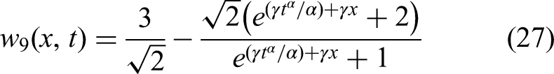
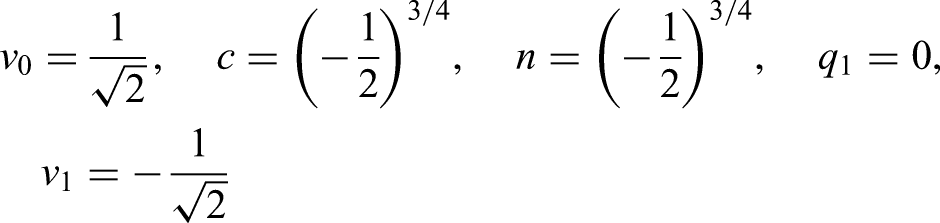
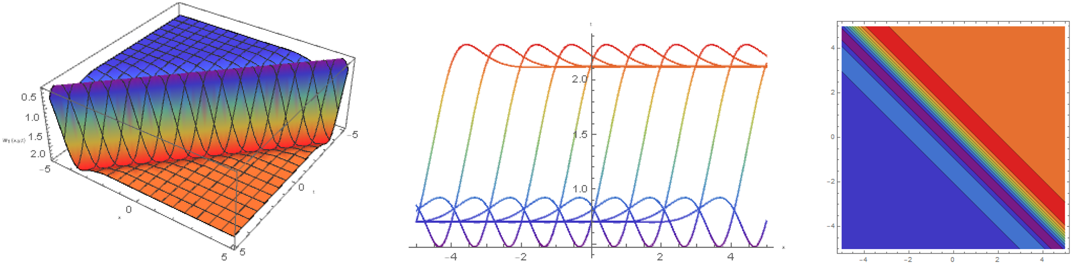
The above shows 3D, 2D and contour figures show the graphically behavior of equation (25) which parameters using values: $v_{0} = - i / \sqrt{2}$ , $c = - \sqrt[4]{- 2}$ , $n = - \sqrt[4]{- 2}$ , $v_{1} = - 1 / \sqrt{2}$ , $q_{1} = 0$ , and $α = 1.$ 3D: three-dimensional; 2D: two-dimensional.

Figure 4.

The above 3D, 2D and contour figures show the graphically behavior of equation (27) which parameters using values: $v_{0} = 3 / \sqrt{2}$ , $c = \sqrt[4]{- 2}$ , $n = \sqrt[4]{- 2}$ , $v_{1} = - \sqrt{2}$ , and $q_{1} = 0$ ; $α = 1.$ 3D: three-dimensional; 2D: two-dimensional.

Figure 5.

The above shows 3D, 2D and contour figures show the graphically behavior of equation (29) which parameters using values: $v_{0} = - 3 / \sqrt{2}$ , $c = \sqrt[4]{- 2}$ , $n = \sqrt[4]{- 2}$ , $v_{1} = \sqrt{2}$ , $q_{1} = 0$ , and $α = 1.$ 3D: three-dimensional; 2D: two-dimensional.

Figure 6.

The above shows 3D, 2D and contour figures show the graphically behavior of equation (31) which parameters using values: $v_{0} = 1 / \sqrt{2}$ , $c = (- 1 / 2)^{3 / 4}$ , $n = (- 1 / 2)^{3 / 4}$ , $q_{1} = 0$ , $v_{1} = - 1 / \sqrt{2}$ , and $α = 1.$ 3D: three-dimensional; 2D: two-dimensional.

The diagram’s main characteristic is a strong localized peak that appears across the surface in a diagonal orientation. In this context, a soliton entity demonstrates the key characteristics. Solitons represent self-sustaining single waves that retain their wave form and velocity when they propagate. The Rosenau equation creates solutions that behave like solitons. The visual illustration on the graph represents an answer to the Rosenau equation. 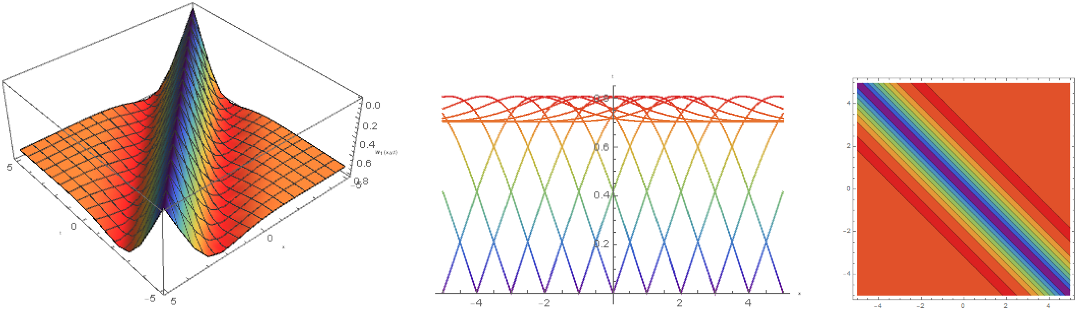A dimensional representation of the $x$ , $t$ , and $w_{1}$ axes depicts a 3 + 1-dimensional solution, where $x$ and $t$ refer to space–time measurements and $w_{1}$ signifies the wave amplitude level. The Rosenau equation allows an extension to multiple dimensions.

The depicted image indicates that a distinct solution type exists for the Rosenau equation, which could manifest as either periodic waves or cnoidal waves. The graphical presentation reveals two independent surfaces that distinguish themselves from each other. The diagram displays a blue-colored flat surface that remains horizontal on top. The lower part of the visual reveals a textured waveform, which displays color gradients. The bottom part of the image reveals periodic wave patterns across a single horizontal axis, which most likely corresponds to the “ $x$ ”-axis. The wave amplitude levels in the bottom figure remain steady across the “ $t$ ”-direction.

A cnoidal wave solution can be identified through the periodic waves with constant amplitude found on the lower surface. Periodic nonlinear waves, which usually solve the Rosenau equation alongside several NLPDEs, constitute the definition of cnoidal waves.

The different surface patterns show potentially overlapping relations between solutions of the Rosenau equation. The flat part represents a uniform solution, but the corrugated area presents itself through cnoidal or periodic solution patterns.

The different parameters used for solution creation in this case differ from those used previously. The selection of different parameter values in NLPDEs will produce completely different solution patterns.

Results and discussion

The use of GERFM incorporating conformable fractional derivatives in the Rosenau equation has yielded a luxuriant family of exact analytical solutions. The solutions are characterized by dark solitons, bright solitons, kink waves, and anti-kink waves that exist in forms of different functions, such as trigonometric, hyperbolic, and exponential functions. Through the systematic alteration of parameters within the GERFM framework, we are able to obtain a range of nonlinear waveform profiles that underscore the potential of the approach and the adaptability of the Rosenau model in describing intricate physical phenomena.

The most significant result is the free parameter sensitivity of the results obtained, especially $n$ and $c$ . These parameters are of utmost importance in establishing the stability, amplitude, and shape of the resultant waves. As an example, varying the values of parameters can produce bright or dark solitons, while varying the parameter sets can produce kink or anti-kink wave structures. This flexibility illustrates the applicability of fractional dynamics to broaden the space of solutions and allow more efficient modeling of nonlinear physical systems.

The graphical solution provides additional evidence for the analytical results. The identification of the resulting solutions is clear-cut: Figure 1 is an anti-kink wave, Figure 2 is a kink wave, Figure 3 is a dark soliton, Figure 4 is a bright soliton, Figure 5 is an anti-kink wave, and Figure 6 is a kink wave. All the figures capture the localized and autopropagating nature of these nonlinear waves, corroborating their solitonic property in the fractional Rosenau model. The soliton solutions retain structure and form, whereas kink and anti-kink waves reaffirm the model’s ability to capture step-like or transitional waveforms typical of the majority of physical environments.

In general, the findings highlight GERFM’s capability for exact and diverse solutions of the Rosenau equation. The finding of various soliton and kink-type solutions highlights the theoretical significance of this method for nonlinear wave analysis. Outside of theory, the results hold potential for plasma physics, fluid dynamics, and materials science applications, where solitons and kinks are involved in wave propagation, energy transfer, and stability of nonlinear systems. By combining fractional calculus with GERFM, the study offers methodological innovation along with new insights into the complex dynamics of nonlinear wave equations.

Conclusion

Solitons for a (3 + 1)-dimensional nonlinear Rosenau equation were obtained in this work using the GERF approach. A close study of a Rosenau equation is important for understanding wave events in many physical systems where nonlinear dynamics and dispersion play a big role. This includes materials science, fluid dynamics, as well as plasma physics. For dense discrete systems, the dynamic behavior has been suggested to be explained by this equation. Three-dimensional graphics have aided in visualizing these solutions, which involve not only trigonometric functions but also hyperbolic and exponential functions, thereby enhancing the understanding of wave dynamics. The exploration of free parameters, along with the results presented, shows their direct influence on wave stability, structure, and interactions, which included but were not limited to the production of M-shaped waves, breaths, kinks, and dark, bright, and isolated wave solutions. Results demonstrate that advanced mathematical methods, such as the GERF method, can solve highly nonlinear wave equations very effectively. These insights not only provide future world theoretical knowledge but also have industrial applications in areas such as plasma physics, ocean engineering, and hydrodynamics. The paper highlights the essentiality of mathematical methods employed to assess problematic physical systems. It also provides a launchpad into an extensive study of nonlinear wave phenomena and their various applications.

Footnotes

ORCID iD

Baboucarr Ceesay

Funding

The authors received no financial support for the research, authorship, and/or publication of this article.

Declaration of conflicting interests

The authors declared no potential conflicts of interest with respect to the research, authorship, and/or publication of this article.

References

Abdou

. The extended tanh method and its applications for solving nonlinear physical models. Appl Math Comput 2007; 190: 988–996.

Liu

Osman

. Nonlinear dynamics for different nonautonomous wave structures solutions of a 3D variable-coefficient generalized shallow water wave equation. Chin J Phys 2022; 77: 1618–1624.

Merdan

. He’s variational iteration method for solving modelling the pollution of a system of lakes. J Sci Technol Dumlupınar Univ 2009; 18: 59–70.

Ghazanfar

Ahmed

Iqbal

, et al. Analysis of multi-wave solitary solutions of (2+1)-dimensional coupled system of Boiti–Leon–Pempinelli. Sci Rep 2024; 14: 20234.

Adomian

. Solving frontier problems of physics: The decomposition method (Vol. 60). Dordrecht: Springer Science & Business Media, 2013.

Iqbal

Inc

Ghazanfar

, et al. Existence and regularity of shock-effected solitons for nonlinear problems in electro-cardiac-physiology. Int J Wavelets Multiresolut Inf Process 2023; 21: 2250053.

Ghazanfar

Macías-Díaz

Sajid Iqbal

, et al. Traveling-wave solutions for a nonlinear non-Ohmic cardio-electro-physiological tissue conduction cable equation. Math Methods Appl Sci 2023; 46: 12690–12710.

Novikov

Manakov

Pitaevskii

, et al. Theory of solitons: The inverse scattering method. Dordrecht: Springer Science & Business Media, 1984.

Ghazanfar

Ahmed

Ali

, et al. Exact and solitary wave structure of the tumor cell proliferation with LQ model of three dimensional PDE by newly extended direct algebraic method. AIP Adv 2023; 13: 125218.

10.

Ghazanfar

Ahmed

Iqbal

, et al. Imaging ultrasound propagation using the Westervelt equation by the generalized Kudryashov and modified Kudryashov methods. Appl Sci 2022; 12: 11813.

11.

Shahid

Baber

Shaikh

, et al. Dynamical study of groundwater systems using the new auxiliary equation method. Results Phys 2024; 58: 107444.

12.

Rahman

Al-Amin

Kamrunnaher

, et al. Mathematical analysis of some new adequate broad-ranging soliton solutions of nonlinear models through the recent technique. Partial Differ Equations Appl Math 2024; 9: 100634.

13.

Al-Amin

Islam

İlhan

, et al. Solitary wave solutions to the modified Zakharov–Kuznetsov and the (2+1)-dimensional Calogero–Bogoyavlenskii–Schiff models in mathematical physics. J Math 2022; 2022: 5224289.

14.

Shahzad

Baber

Ahmad

, et al. On the analytical study of predator–prey model with Holling-II by using the new modified extended direct algebraic technique and its stability analysis. Results Phys 2023; 51: 106677.

15.

Ceesay

Yasin

Ahmed

, et al. Revealing homoclinic breather waves, periodic lump waves and other waves forms of an integrable reduced spin Hirota–Maxwell–Bloch system. Sci Rep 2025; 15: 19880.

16.

Ceesay

Baber

Ahmed

, et al. Harvesting mixed, homoclinic breather, M-shaped, and other wave profiles of the Heisenberg ferromagnet-type Akbota equation. Eur J Pure Appl Math 2025; 18: 5851–5851.

17.

Afrin

. Solitary wave solutions and investigation the effects of different wave velocities of the nonlinear modified Zakharov–Kuznetsov model for the wave propagation in nonlinear media. Partial Differ Equations Appl Math 2023; 8: 100583.

18.

Islam

Al-Amin

Akbar

, et al. Assorted optical soliton solutions of the nonlinear fractional model in optical fibers possessing beta derivative. Phys Scr 2023; 99: 015227.

19.

Baber

Mohammed

Ahmed

, et al. Exact solitary wave propagations for the stochastic Burgers’ equation under the influence of white noise and its comparison with computational scheme. Sci Rep 2024; 14: 10629.

20.

Ahmed

Ghazanfar

Baber

, et al. Analytical solutions and implications for hydrodynamics and nonlinear optics. AIP Adv 2025; 15: 85004.

21.

Chen

. Numerical approaches to fractional calculus and fractional ordinary differential equation. J Comput Phys 2011; 230: 3352–3368.

22.

Tricomi

. Integral equations (Vol. 5). New York: Courier Corporation, 1985.

23.

Park

. On the Rosenau equation. Math Appl Comput 1990; 9: 145–152.

24.

Ceesay

Baber

Ahmed

, et al. Breather, lump and other wave profiles for the nonlinear Rosenau equation arising in physical systems. Sci Rep 2025; 15: 3067.

25.

Park

. Pointwise decay estimates of solutions of the generalized Rosenau equation. J Korean Math Soc 1992; 29: 261–280.

26.

Atouani

Omrani

. A new conservative high-order accurate difference scheme for the Rosenau equation. Appl Anal 2015; 94: 2435–2455.

27.

Gao

Tian

. Lie symmetry reductions and exact solutions to the Rosenau equation. Adv Math Phys 2014; 2014: 714635.

28.

Abbaszadeh

Dehghan

. The two-grid interpolating element free Galerkin (TG-IEFG) method for solving Rosenau-regularized long wave (RRLW) equation with error analysis. Appl Anal 2018; 97: 1129–1153.

29.

Avazzadeh

Nikan

Machado

JAT

. Solitary wave solutions of the generalized Rosenau–KdV–RLW equation. Mathematics 2020; 8: 1601.

30.

Zuo

. Solitons and periodic solutions for the Rosenau–KdV and Rosenau–Kawahara equations. Appl Math Comput 2009; 215: 835–840.

31.

Shi

Jia

. Super convergence analysis of the mixed finite element method for the Rosenau equation. J Math Anal Appl 2020; 481: 123485.

32.

Karakoc

Biswas

. Numerical scheme to dispersive shallow water waves. J Comput Theor Nanosci 2016; 13: 7084–7092.

33.

Razborova

Moraru

Biswas

. Perturbation of dispersive shallow water waves with Rosenau–KdV–RLW equation and power law nonlinearity. Rom J Phys 2014; 59: 658–676.

34.

Battal Gazi Karakoc

Triki

. Numerical simulation for treatment of dispersive shallow water waves with Rosenau–KdV equation. Eur Phys J Plus 2016; 131: 356.

35.

Erbay

Erkip

. Numerical computation of solitary wave solutions of the Rosenau equation. Wave Motion 2020; 98: 102618.

36.

Guo

Wang

Luo

. A conservative and implicit second-order nonlinear numerical scheme for the Rosenau–KdV equation. Mathematics 2021; 9: 1183.

37.

Chunk

Pani

. Numerical methods for the Rosenau equation: Rosenau equation. Appl Anal 2001; 77: 351–369.

38.

Omrani

Abidi

Achouri

, et al. A new conservative finite difference scheme for the Rosenau equation. Appl Math Comput 2008; 201: 35–43.

39.

Alotaibi

Althobaiti

. Exact wave solutions of the nonlinear Rosenau equation using an analytical method. Open Phys 2021; 19: 889–896.

40.

Shakeel

Shah

Chung

. Novel analytical technique to find closed form solutions of time fractional partial differential equations. Fractal Fract 2022; 6: 24.

41.

Mumtaz

Shakeel

Manan

, et al. Stability and chaotic analysis of nonlinear fractional model using novel analytical technique: Soliton solutions for Wazwaz Kaur Boussinesq equation. Rev Int Metod Numer Calc Diseno Ing 2025; 41: 27.

42.

Shakeel

. Investigating the DNA Peyrard–Bishop model by beta derivatives using new analytical technique. Int J Biomath 2025; 2550027.

43.

Shakeel

Manan

Turki

, et al. Novel analytical technique to find diversity of solitary wave solutions for Wazwaz–Benjamin–Bona Mahony equations of fractional order. Results Phys 2023; 51: 106671.

44.

Almatrafi

. Solitary wave solutions to a fractional-order Fokas equation via the improve modified extended tanh-function approach. Mathematics 2024; 13: 109.

45.

Alzubaidi

Almatrafi

. Stability and closed-form soliton solutions for the space–time fractional symmetric regularized long wave equation via two effective approaches. Mod Phys Lett B 2025; 39: 2550201.

46.

Almatrafi

. Abundant traveling wave and numerical solutions for Novikov–Veselov system with their stability and accuracy. Appl Anal 2023; 102: 2389–2402.

47.

Alzubaidi

Almatrafi

. New soliton solutions to the space–time fractional Boussinesq equation using a reliable method. Int J Anal Appl 2024; 22: 135–135.

48.

Almatrafi

. Solitary wave solutions to a fractional model using the improved modified extended tanh-function method. Fractal Fract 2023; 7: 252.

49.

Almatrafi

. Construction of closed form soliton solutions to the space–time fractional symmetric regularized long wave equation using two reliable methods. Fractals 2023; 31: 2340160.

50.

Berkal

Almatrafi

. Bifurcation and stability of two-dimensional activator–inhibitor model with fractional-order derivative. Fractal Fract 2023; 7: 344.

51.

Almatrafi

Alzubaidi

Berkal

. Bifurcation analysis, phase portrait, and certain types of solutions to the space–time fractional Sharma–Tasso–Olver equation using reliable methods. J Appl Math Comput 2025; 71: 1–22.

52.

Ali

Ahmad

Javed

, et al. Investigate the dynamic nature of soliton solutions and bifurcation analysis to a new generalized two-dimensional nonlinear wave equation with its stability. Results Phys 2023; 53: 106922.

53.

Kaplan

Alqahtani

. Exploration of new solitons for the fractional perturbed Radhakrishnan–Kundu–Lakshmanan model. Mathematics 2023; 11: 2562.

54.

Jannat

Raza

Kaplan

, et al. Dynamics of lump, breather, two-waves and other interaction solutions of (2+1)-dimensional KdV equation. Int J Appl Comput Math 2023; 9: 125.

55.

Abdeljawad

. On conformable fractional calculus. J Comput Appl Math 2015; 279: 57–66.

56.

Shahzad

Ahmad

Baber

, et al. Extraction of soliton for the confirmable time-fractional nonlinear Sobolev-type equations in semiconductor by

ϕ^{6}

-modal expansion method. Results Phys 2023; 46: 106299.

Nonlinear wave dynamics and soliton solutions of the Rosenau equation with conformable fractional derivatives

Abstract

Keywords

Introduction

Preliminaries of conformable derivatives

The technique

Application of the method

Solution sets

Family 1 of the solutions of equation (1)

Family 2 of the solutions of equation (1)

Family 3 of the solutions of equation (1)

Family 4 of the solutions of equation (1)

Family 5 of the solutions of equation (1)

Family 6 of the solutions of equation (1)

Family 7 of the solutions of equation (1)

Family 8 of the solutions of equation (1)

Family 9 of the solutions of equation (1)

Family 10 of the solutions of equation (1)

Family 11 of the solutions of equation (1)

Graphical behavior

Results and discussion

Conclusion

Footnotes

ORCID iD

Funding

Declaration of conflicting interests

References