Approximate solutions of Korteweg-de Vries-Benjamin-Bona-Mahony-Burgers equation with dissipative terms

Abstract

In this paper, the Korteweg-de Vries-Benjamin-Bona-Mahony-Burgers (KdV-BBM-B) equation is investigated which plays an essential role in numerous subjects of engineering and science. Using the theory of planar dynamical systems, we qualitatively analyze the bounded traveling wave solutions of the KdV-BBM-B equation. The conditions about the presence of bounded traveling wave solutions are obtained resoundingly. Meanwhile, the relationships between the waveform of the bounded traveling wave solution and the dissipation coefficient γ are investigated. Furthermore, when the absolute value of the dissipation coefficient γ is bigger than the critical value, the equation has a kink solitary wave solution. Nevertheless, when |γ| is less than the critical value, the solution has oscillatory and damped properties. According to the evolution relations of orbits in the global phase portraits which the damped oscillatory solutions correspond to, by using undetermined coefficients method, we obtain the approximate damped oscillatory solutions with a bell head and oscillatory tail, and the approximate damped oscillatory solutions with a kink head and oscillatory tail. By the idea of homogenization principle, we give the error estimates for these approximate solutions by establishing the integral equations reflecting the relations between approximate damped oscillatory solutions and their exact solutions. The errors are infinitesimal decreasing in the exponential form. Finally, to better understand the dynamics of the oscillatory damped solution, we give a graphical analysis of the effect of the dissipation coefficient γ on it.

Introduction

As is known to all that nonlinear wave equations (NLWEs) are fundamental physical models which have been applied in various fields, especially in physics.

The problem of solving NLWEs is an ancient and important research topic. Although many scholars have done a lot of work on solving the problem, due to the complexity of NLWE itself, the solutions that can be obtained are only a small part of the implication of NLWE itself, and NLWEs that can be solved accurately are also very few. Therefore, in the process of studying the solution of NLWE, it is mainly studied from two aspects: the exact solution and the approximate solution.

Solutions in different forms are the most interesting research points of NLWEs. ¹ In order to research NLWEs that model wave phenomena, the traveling wave solution should be studied first. Traveling wave solution plays a very important role in nonlinear science, they can well describe various natural phenomena, such as vibrations, propagating waves, and solitons. Traveling wave solution is a solution of permanent form moving with a constant velocity. There are many types of traveling wave solutions that are of particular interest in solitary wave theory that is rapidly developing in many scientific fields from water waves in shallow water to plasma physics. However, not all equations can be solved by a certain method, so it often requires clever construction by the researcher when studying.^2,3 A variety of powerful methods have been developed to study traveling wave solution such as Hirota bilinear method,^4,5 inverse scattering transformation,^6,7 Darboux transformation and Bäcklund transformation^8–10 and so on.^11–18 In addition, there is a kind of method that based on the theory of planar dynamical systems. This method mainly uses the bifurcation theory of the dynamic system and combines with the phase diagram of integrable wave system, many exact traveling wave solutions have been obtained using elliptic functions as well as other tools.

In recent years, Li and Zhang ¹⁹ constructed the first integration method combined with phase diagram analysis by using the characteristics of Hamilton system. After that, Shen et al. ²⁰ continued to promote and develop this method to find the possible bounded traveling wave solution of the equation.

After all, there are few equations that can be solved accurately. In order to study the rich characteristics of the equation itself, researchers have to take the approximate solution method. Adomian decomposition method^21,22 and Padé approximation method ²³ have been developed to solve the nonlinear wave equation approximately. Recently, He has applied variational iteration method^24,25 and the homotopy perturbation method ²⁶ to the solution of wave equations. Liao et al.^27,28 applied homotopy analysis method to the approximate solution of wave equation. Shen et al. ²⁹ used the qualitative theory of differential equation to construct the approximate solution of the equation according to the characteristics of the orbit near the equilibrium point combined with the method of computer symbolic algebra, all of which achieved good results.

Since Poincaré, a famous French mathematician, used qualitative theory to study dynamical systems, the theory of dynamical systems has made great progress, and it has penetrated into various branches of mathematics.

The study of NLWEs focus on the evolution of waves over time, particularly solitary waves in equation. In fact, it is a special coherent structure, which is a limit state for the traveling wave solution of NLWEs. Very recent and related research works are included such as Mohammed et al. (2021), Baber et al (2024), Mohammed et al. (2022), Alshammari et al. (2022).^30–33 It can be analyzed as homoclinic or heteroclinic orbits of the ordinary differential equation that characterizes the traveling wave solution.

Because wave comes across the damping in the movement, dissipation would rise. G.B. Whitham ³⁴ pointed out that one of basic problems which need to be concerned for nonlinear evolution equations is how dissipation affects nonlinear system. Therefore, motivated by this question, the main purpose of this paper is to make a qualitative analysis of the KdV-BBM-B equation in the form ³⁵ .

$\begin{array}{c}\hfill u_t+\alpha u_x+\beta u{u}_x+\gamma u_{xx}-\mu u_{\mathit{xxt}}+\delta u_{\mathit{xxx}}=0,x\in \mathrm{\Omega }=[a,b],t\in [0,T],\hfill \end{array}$

(1.1)

with the initial condition u (x, 0) = f(x), and boundary conditions u (a, t) = u (b, t) = 0, where α, β, μ and δ are positive real constants, γ ≥ 0, and u represents the free surface elevation above the still water level u = 0. The KdV-BBM-Burgers equation is a significant mathematical and physical model for depicting the propagation of weakly nonlinear dispersive long waves under dissipative influences. By integrating the features of the KdV equation, the BBM equation, and the Burgers equation, this equation is applicable to describe a variety of physical phenomena, such as the propagation of water waves and gas dynamics. This equation is extensively utilized in physics, engineering, and mathematics. For instance, in the theory of water waves, it can be employed to model the wave propagation in deep water; in aerodynamics, it can be used to describe the motion of viscous fluids. In recent years, through constructing a new functional space and using Bourgain space theory, researchers have conducted in-depth studies on the existence of the adaptive solution of the equation and obtained numerous significant results. To summarize, the Korteweg-de Vries-Benjamin-Bona-Mahony-Burgers equation is a mathematical model that integrates multiple physical effects, which possesses a broad application background and significant research value.

Equation (1.1) is a complex equation that integrates the characteristics of several classical nonlinear partial differential equations and is extensively applied in the domains of fluid mechanics, nonlinear acoustics, and gas dynamics. This equation possesses a remarkable advantage in depicting nonlinear wave phenomena in fluids. The capacity of equation (1.1) to account for both dispersion and dissipation effects is pivotal for comprehending the wave behavior in complex fluid systems. In the realm of nonlinear acoustics, equation (1.1) can be utilized to model the propagation of sound waves in nonlinear media, particularly when considering the nonlinear interactions and dissipative effects of sound waves. Although equation (1.1) was not initially intended for gas dynamics, its nonlinear properties and dissipation term render it potentially applicable in the simulation of certain compressible fluid flows. With appropriate modification and extension, equation (1.1) might be employed to describe the complex flow phenomena of gases in the boundary layer, such as nonlinear fluctuations and energy dissipation in the turbulent boundary layer. When α, β, μ, δ, and γ take some given values, equation (1.1) may be reduced to other famous nonlinear model equations in physics. For α = γ = μ = 0 and β = 6, δ = 1, equation (1.1) converts to the KdV equation ³⁶ .

$u_t+6u{u}_x+u_{\mathit{xxx}}=0.$

(1.2)

The KdV equation arises in the study of shallow water waves. In particular, the KdV equation is used to describe long waves traveling in canals. Since 1960s, with the deepening of research on nonlinear phenomena, it has been discovered that there exists a broad class of wave equations or equations describing nonlinear interactions, which can be reduced to the KdV equation. For instance, these include magnetocurrent waves in plasma, ionic sound waves, non-resonant lattice vibrations, pressure waves in liquid-gas mixtures, and thermal excitation of phonon packets in nonlinear lattices at low temperatures. Therefore, the KdV equation represents a significant development in understanding important nonlinear phenomena in science.

If α = δ = μ = 0 and β = 1, γ = −1, then equation (1.1) reduces to the Burgers equation ³⁷

$\begin{array}{c}\hfill u_t+u{u}_x-u_{xx}=0.\hfill \end{array}$

(1.3)

Among the nonlinear development equations, Burgers equation is a representative dissipative wave equation. It is the simplest nonlinear diffusion wave model, derives from the theory of turbulence research. Burgers equations can describe a wide range of physical phenomena, such as sound waves in a viscous medium, magnetic currents with limited conductance, and waves in a fluid-filled viscoelastic tube.

If γ = δ = 0 and α = μ = β = 1, equation (1.1) becomes the BBM equation ³⁸

$\begin{array}{c}\hfill u_t+u_x+u{u}_x-u_{\mathit{xxt}}=0.\hfill \end{array}$

(1.4)

This equation is crucial in physics media as it defines a great number of phenomena with weak nonlinearity and dispersion waves, involving on acoustic waves and magnetohydrodynamics waves in plasmas, longitudinal dispersive waves in elastic rods, pressure waves in liquid gas bubbles, nonlinear transverse waves in shallow water, optical fibers, etc.

If γ ≠ 0, the equation (1.1) exists a dissipative effect. Because dissipation is unavoidable in practice, Zhang investigated a number of NLWEs with dissipative effect and obtained exact bounded traveling wave and approximate oscillatory damped solutions.^39–43 Tian analyzed bounded traveling wave solution of (2 + 1)-dimensional breaking soliton equation. ⁴⁴ Very recent and some related work of the research on solitary wave solutions and dynamical behaviors such as.^45–50 However, we will investigate the effect of the dissipation coefficient γ and find an accurate or approximate oscillatory damped solution as well as their error estimate. To the best of our knowledge, the problem about bounded traveling wave solutions of the equation (1.1) on the basis of the theory of planar dynamical systems has not been reported yet.

The outline of this paper is as follows. Firstly, we make a qualitative analysis of the dynamic system corresponding to (1.1). The conditions for the existence of global phase diagrams and bounded traveling wave solutions with different parameters are discussed. Then, the relation between the waveform of the bounded traveling wave solution of the equation (1.1) and the dissipation coefficient γ is expressed. Furthermore, we construct the bell profile solitary wave solutions and kink profile solitary wave solutions of the equation (1.1) by using the method of undetermined coefficients. Meanwhile, the approximate vibration damping solutions under two different conditions are given. Finally, we derive an error estimate and discussions of the approximate oscillatory damping solution of (1.1). The sixth part is the conclusion and prospect of this paper.

Qualitative analysis of bounded traveling wave solutions

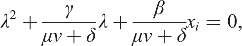
It is evident that the traveling wave solutions u (x, t) = u(ξ) = u (x − vt) of equation (1.1) satisfy

$\begin{array}{c}\hfill (-v+\alpha )u(\xi )+\frac{\beta }{2}{u}^2(\xi )+\gamma u^{\prime }(\xi )+(\mu v+\delta )u^{\prime \prime }(\xi )-k=0,\hfill \end{array}$

(2.1)

as u′(ξ), u′′(ξ), u′′′(ξ) → 0, |ξ| → +∞, lim_ξ→±∞u(ξ) = u (±∞), where k is an integral constant. Setting U(ξ) = u(ξ) − $\frac{v-\alpha }{\beta }$ in (2.1) yields

$\begin{array}{c}\hfill U^{\prime \prime }(\xi )+\frac{\gamma }{\mu v+\delta }{U}^{\prime }(\xi )+\frac{\beta }{2(\mu v+\delta )}{U}^2(\xi )-\frac{{(v-\alpha )}^2+2k\beta }{2\beta (\mu v+\delta )}=0.\hfill \end{array}$

(2.2)

Let x = U(ξ), y = U′(ξ), then (2.2) can be reduced to the following planar dynamical system:

$\left\{\begin{array}{cc}\hfill & \frac{dx}{d\xi }=y\equiv P(x,y),\hfill \\ \hfill & \frac{dy}{d\xi }=\frac{-\gamma }{\mu v+\delta }y-\frac{\beta }{2(\mu v+\delta )}\left(x^2-\frac{{(v-\alpha )}^2+2k\beta }{{\beta }^2}\right)\equiv Q(x,y).\hfill \end{array}\right.$

(2.3)

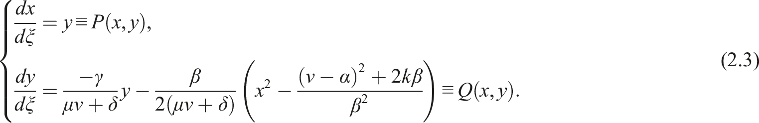
The orbits of the planar dynamical system (2.3) is related to the solutions of equation (1.1) as follows:

The homoclinic orbit and closed orbit of (2.3) corresponding to bell profile solitary wave solution and periodic traveling wave solution of equation (1.1), respectively; A heteroclinic orbit of (2.3) may correspond to a monotone kink profile solitary wave solution or a non-monotone bounded traveling wave solution of (1.1).

Therefore, in order to search for the bounded traveling wave solution of equation (1.1), we just need to investigate the bounded orbits of the planar dynamical system (2.3). To achieve this, we study (2.3) using the theory of planar dynamical systems.^51–53

Proposition 1

When γ ≠ 0, planar dynamical system (2.3) does not exist any closed orbit or singular closed orbit with finite singular points on the (x, y) phase plane. So, equation (1.1) has neither periodic traveling wave solutions nor bell profile solitary wave solutions as γ ≠ 0.

Proof For ∂P/∂x + ∂Q/∂y = −γ/μv + δ, on the basis of Bendixson–Dulac criterion^51–53 Proposition 1 is established when γ ≠ 0.

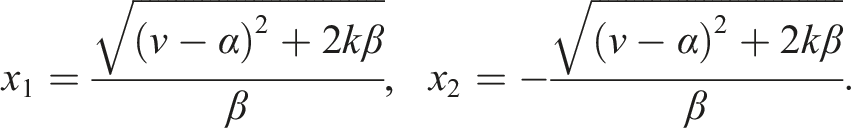
It is obvious that system (2.3) exists two different singular points P _i (x _i , 0) (i = 1, 2) under the conditions assumed of (v − α)² + 2kβ > 0, in which

$\begin{array}{c}\hfill x_1=\frac{\sqrt{{(v-\alpha )}^2+2k\beta }}{\beta },x_2=-\frac{\sqrt{{(v-\alpha )}^2+2k\beta }}{\beta }.\hfill \end{array}$

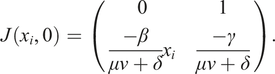
The Jacobian matrix of system (2.3) at P _i (x _i , 0) (i = 1, 2) are marked as

$\begin{array}{c}\hfill J(x_i,0)=\left(\begin{array}{cc}\hfill 0\hfill & \hfill 1\hfill \\ \hfill \frac{-\beta }{\mu v+\delta }{x}_i\hfill & \hfill \frac{-\gamma }{\mu v+\delta }\hfill \end{array}\right).\hfill \end{array}$

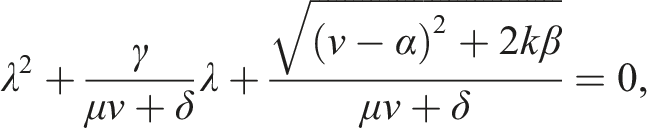
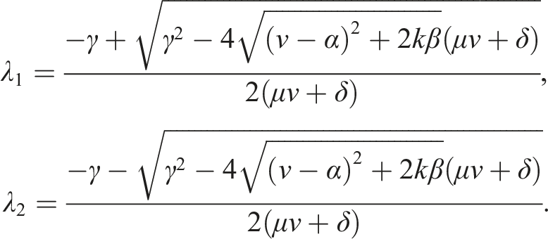
Then the characteristic equations of the linearized system corresponding to (2.3) at P _i (x _i , 0) (i = 1, 2) are

$\begin{array}{c}\hfill {\lambda }^2+\frac{\gamma }{\mu v+\delta }\lambda +\frac{\beta }{\mu v+\delta }{x}_i=0,\hfill \end{array}$

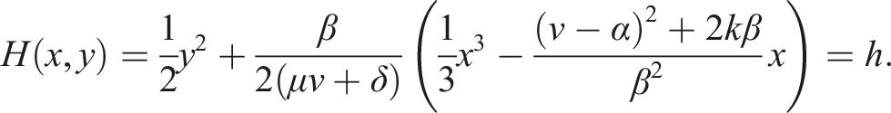
its discriminant is Δ _i = γ²/(μv + δ)² − 4β/μv + δx _i . According to the theory of planar dynamical systems, we can draw the following conclusions:

• (1) P₂ (x₂, 0) is a saddle point.

• (2) When γ = 0, P₁ (x₁, 0) is a center (see Figure 1(a)) on account of planar dynamical system (2.3) exists the first integral

  $\begin{array}{c}\hfill H(x,y)=\frac{1}{2}{y}^2+\frac{\beta }{2(\mu v+\delta )}\left(\frac{1}{3}{x}^3-\frac{{(v-\alpha )}^2+2k\beta }{{\beta }^2}x\right)=h.\hfill \end{array}$

• (3) When γ(μv + δ) < 0, P₁ (x₁, 0) is an unstable node point (see Figure 1(b)) as Δ₁ > 0 and it is an unstable focus point (see Figure 1(d)) as Δ₁ < 0.

• (4) When γ(μv + δ) > 0, P₁ (x₁, 0) is a stable node point (see Figure 1(e)) as Δ₁ > 0 and it is a stable focus point (see Figure 1(c)) as Δ₁ < 0.

  Figure 1.

  Global phase diagrams. (a) γ = 0, (b) γ(μv + δ) < 0, Δ₁ > 0, (c) γ(μv + δ) > 0, Δ₁ < 0, (d) γ(μv + δ) < 0, Δ₁ < 0, (e) γ(μv + δ) > 0, and Δ₁ > 0.

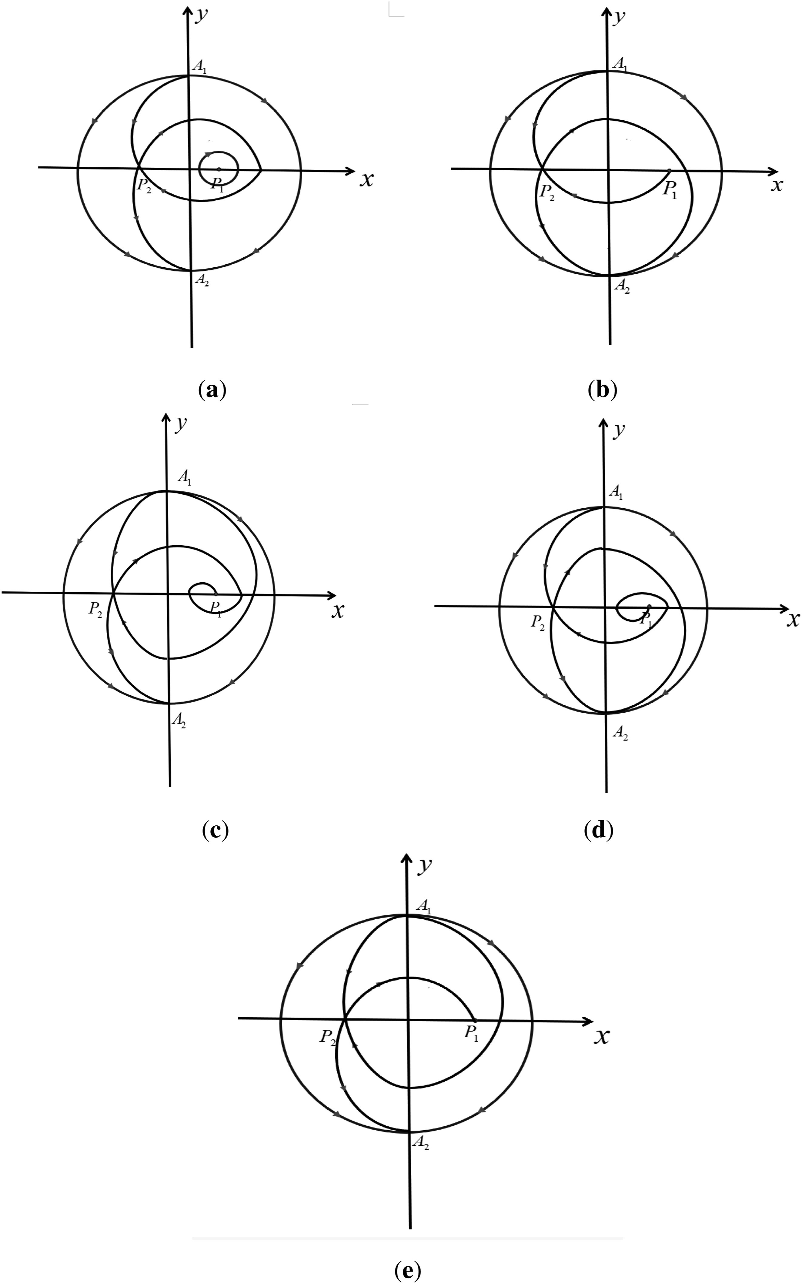
Obviously, there are two singular points A _i (i = 1, 2) at the infinity on the y-axis on the basis of the analysis of Poincaré transformation to system (2.3). In which A₁ is a souse point on the positive y-axis and A₂ is a sink point on the negative y-axis. What is more, the circumference of the Poincaré disc is a singular closed orbit as well.Based on the qualitative discussion, we present the global phase diagrams of planar dynamical system (2.3) in Figures 1(a)–(e).

Proposition 2

(i) If γ = 0 and (v − α)² + 2kβ > 0, then apart from singular points P₁, P₂ and the orbit L(P₁, P₁) and L(P₂, P₂), all non-periodic orbits of (2.3) are unbounded. Furthermore, the coordinate values of the orbits tend to infinity.

(ii) If γ(μv + δ) > 0 (γ(μv + δ) < 0) and (v − α)² + 2kβ > 0, then except for singular points P₁, P₂ and orbit L (P₂, P₁) (L (P₁, P₂)), all non-periodic orbits of (2.3) are unbounded. Furthermore, the coordinate values of the orbits tend to infinity.

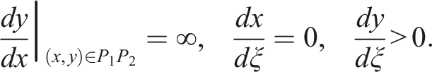
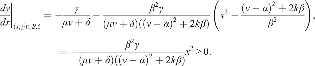
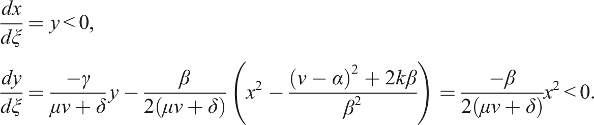
Proof. When (v − α)² + 2kβ > 0 and γ = 0, it’s not difficult to prove that all non-periodic orbits are unbounded. As a matter of fact, when |ξ| → ∞, these non-periodic orbits tend to either A₁ or A₂; therefore, the ordinate values of these non-periodic orbits approach infinity as |ξ| → ∞. Suppose that the abscissa values of these orbits are bounded. The tangent slope of the orbits at any point satisfies.

$\begin{array}{c}\hfill \frac{dy}{dx}=-\frac{\beta }{2(\mu v+\delta )y}\left(x^2-\frac{{(v-\alpha )}^2+2k\beta }{{\beta }^2}\right),\hfill \end{array}$

$\frac{dy}{dx}$ → 0, when y → ∞. However, $\frac{dy}{dx}$ cannot maintain bounded as y → ∞ by the differential mean value theorem. It means that abscissa values of points on these non-periodic orbits tend to infinity as |ξ| → ∞. The deduction (ii) could be proved similarly.

Because of the relationship between (1.1) and (2.3), we establish the following theorem from Proposition 2 and Figures 1(a)–(e).

Theorem 1

Assuming that the wave speed v and integral constant k satisfy (v − α)² + 2kβ > 0.

(i) In the case where γ = 0, there are infinitely many periodic traveling wave solutions and a bell profile solitary wave solution in Equation (1.1) that corresponds to the homoclinic orbit L (P₂, P₂) in Figure 1(a).

(ii) If γ(μv + δ) > 0 (γ(μv + δ) < 0), then the unique bounded traveling wave solution of Equation (1.1) corresponds to the heteroclinic orbit L (P₂, P₁) in Figures 1(e) and (c), or corresponding to the heteroclinic orbit L (P₁, P₂) in Figures 1(b) and (d).

The relationship between the behaviors of bounded traveling wave solutions and the dissipation coefficient

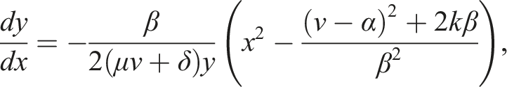
Based on the relationship between (1.1) and (2.3), we can investigate the relationship between the behaviors of bounded traveling wave solutions and the dissipation coefficient γ according to the relationship between the behaviors of bounded orbits of (2.3) and the parameter γ, we construct two theorems as follows.

Theorem 2

Hypothesis that the wave speed v and integral constant k satisfy (v − α)² + 2kβ > 0.(i) If $\gamma <-2\sqrt[4]{({(v-\alpha )}^2+2k\beta )\mathrm{\Delta }}$ , Δ = (μv + δ)² is satisfied by the wave speed v and the dissipation coefficient γ, then (1.1) indicates that there is only one monotone decreasing kink profile solitary-wave solution u(ξ) that corresponds to the heteroclinic orbit L (P₁, P₂) in Figure 1(b) and so as to.

$\begin{array}{c}\hfill u(-\infty )=\frac{v-\alpha }{\beta }+x_1,u(+\infty )=\frac{v-\alpha }{\beta }+x_2.\hfill \end{array}$

(3.1)

(ii) When $\gamma <-2\sqrt[4]{({(v-\alpha )}^2+2k\beta )\mathrm{\Delta }}$ , Δ = (μv + δ)² is satisfied by the dissipation coefficient γ and the wave speed v, then (1.1) exists a distinct monotone rising kink profile solitary-wave solution u(ξ) that corresponds to the heteroclinic orbit L (P₂, P₁) in Figure 1(e) so as to

$\begin{array}{c}\hfill u(-\infty )=\frac{v-\alpha }{\beta }+x_2,u(+\infty )=\frac{v-\alpha }{\beta }+x_1.\hfill \end{array}$

(3.2)

Proof

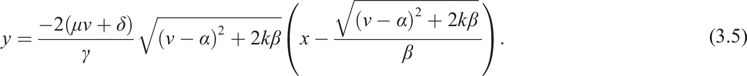
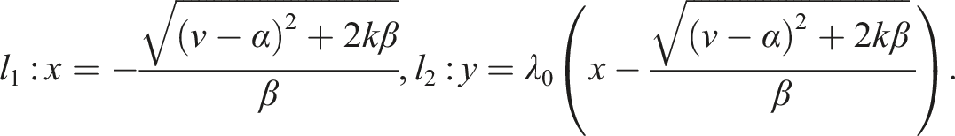
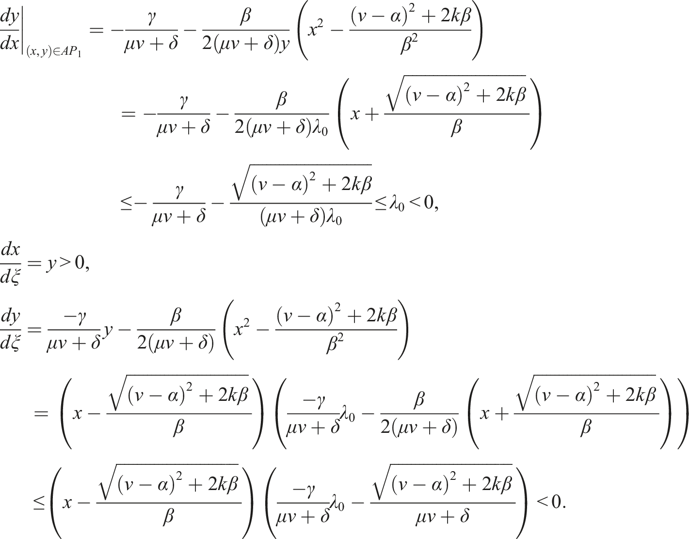
(i) We just need to prove that U′(ξ) ≠ 0 for all ξ ∈ R on account of the relationship between u(ξ) and U(ξ) as well as u(+∞) < u(−∞) when ξ → ±∞. Notice that if there is ξ0 ∈ R meeting U′(ξ₀) = 0, it signifies that there is another intersection point of L(P₁, P₂) and the x-axis besides P₁ and P₂. We prove that this is impossible.

To begin with, we discuss the vector field (2.3) in the (x, y) phase plane. The secondary curve

$\begin{array}{c}\hfill \frac{-\gamma }{\mu v+\delta }y=\frac{\beta }{2(\mu v+\delta )}\left(x^2-\frac{{(v-\alpha )}^2+2k\beta }{{\beta }^2}\right),\hfill \end{array}$

(3.3)

is the whole orbit of vectors paralleling the x-axis (see Figure 2(a)), with its vertex being marked by A with the coordinates (0, ((v − α)² + 2kβ)/2βγ). Drawing a straight line, denoted by l₁, which parallels the x-axis and passes through A, and making another straight line denoted by l₂, which passes through P₁ and its tangent slope,

$\begin{array}{c}\hfill \tan \theta =\frac{-2(\mu v+\delta )}{\gamma }\sqrt{{(v-\alpha )}^2+2k\beta }.\hfill \end{array}$

(3.4)

Namely, l₂ is

$\begin{array}{c}\hfill y=\frac{-2(\mu v+\delta )}{\gamma }\sqrt{{(v-\alpha )}^2+2k\beta }\left(x-\frac{\sqrt{{(v-\alpha )}^2+2k\beta }}{\beta }\right).\hfill \end{array}$

(3.5)

Let B be the intersection point of l₁ and l₂. It is obvious that its abscissa value x _B satisfies $0<x_B<\sqrt{{(v-\alpha )}^2+2k\beta }/\beta$ .

The closed curve with line segments P₂P₁, P₁B, BA, and secondary curve $\widehat{P_{2}A}$ is non-tangential in system (2.3). Integral orbits beginning from outer points cannot reach the region G enclosed by line segments P₂P₁, P₁B, BA, and secondary curve $\widehat{P_{2}A}$ as ξ increases. Taking the coordinate values of points on line segments P₂P₁, P₁B, BA, and secondary curve $\widehat{P_{2}A}$ into system (2.3) yields P₂P₁.

$\begin{array}{c}\hfill \frac{dy}{dx}{|}_{(x,y)\in P_1{P}_2}=\infty ,\frac{dx}{d\xi }=0,\frac{dy}{d\xi }>0.\hfill \end{array}$

On the secondary curve $\widehat{P_{2}A}$

$\begin{array}{ll}\hfill & \frac{dy}{dx}{|}_{(x,y)\in \widehat{P_{2}A}}=-\frac{\gamma }{\mu v+\delta }-\frac{{\beta }^2\gamma }{(\mu v+\delta )({(v-\alpha )}^2+2k\beta )}\left(x^2-\frac{{(v-\alpha )}^2+2k\beta }{{\beta }^2}\right)=0,\hfill \\ \hfill & \frac{dx}{d\xi }=y<0,\hfill \\ \hfill & \frac{dy}{d\xi }=\frac{-\gamma }{\mu v+\delta }y-\frac{\beta }{2(\mu v+\delta )}\left(x^2-\frac{{(v-\alpha )}^2+2k\beta }{{\beta }^2}\right)=0.\hfill \end{array}$

Obviously, P₂P₁ and $\widehat{P_{2}A}$ are generalized non-tangential curves. Next, we certificate that P₁B and BA are generalized non-tangential curves. On the line segment P₁B

$\begin{array}{ll}\hfill & \frac{dy}{dx}{|}_{(x,y)\in P_{1}B}=-\frac{\gamma }{\mu v+\delta }-\frac{\beta }{2(\mu v+\delta )y}\left(x^2-\frac{{(v-\alpha )}^2+2k\beta }{{\beta }^2}\right),\hfill \\ \hfill & =-\frac{\gamma }{\mu v+\delta }-\frac{\beta }{2(\mu v+\delta )y}\left(x-\frac{\sqrt{{(v-\alpha )}^2+2k\beta }}{\beta }\right)\left(x+\frac{\sqrt{{(v-\alpha )}^2+2k\beta }}{\beta }\right),\hfill \\ \hfill & =-\frac{\gamma }{\mu v+\delta }+\frac{\beta }{4\gamma \sqrt{{(v-\alpha )}^2+2k\beta }}\left(x+\frac{\sqrt{{(v-\alpha )}^2+2k\beta }}{\beta }\right),\hfill \\ \hfill & \ge -\frac{\gamma }{2(\mu v+\delta )}\ge -\frac{2(\mu v+\delta )}{\gamma }\sqrt{{(v-\alpha )}^2+2k\beta }=\tan \theta >0.\hfill \end{array}$

The equality can be established if and only if x = x₁. The above formula indicates that the tangent slope of the orbit passing through segment P₁B is greater than that at P₁B, except for point P₁. Now let us continue to consider the direction of the vector field in P₁B as shown below, substituting (3.5) into (2.3), we have

$\begin{array}{ll}\hfill & \frac{dx}{d\xi }=y<0,\hfill \\ \hfill & \frac{dy}{d\xi }=\frac{-\gamma }{\mu v+\delta }y-\frac{\beta }{2(\mu v+\delta )}\left(x^2-\frac{{(v-\alpha )}^2+2k\beta }{{\beta }^2}\right)<0.\hfill \end{array}$

So the orbit drills out of the region D as it passes through segment P ₁ B (see Figure 2(a)). On the line segment BA

$\begin{array}{ll}\hfill & \frac{dy}{dx}{|}_{(x,y)\in BA}=-\frac{\gamma }{\mu v+\delta }-\frac{{\beta }^2\gamma }{(\mu v+\delta )({(v-\alpha )}^2+2k\beta )}\left(x^2-\frac{{(v-\alpha )}^2+2k\beta }{{\beta }^2}\right),\hfill \\ \hfill & =-\frac{{\beta }^2\gamma }{(\mu v+\delta )({(v-\alpha )}^2+2k\beta )}{x}^2>0.\hfill \end{array}$

We think about account the directions of the vector field on BA

$\begin{array}{ll}\hfill & \frac{dx}{d\xi }=y<0,\hfill \\ \hfill & \frac{dy}{d\xi }=\frac{-\gamma }{\mu v+\delta }y-\frac{\beta }{2(\mu v+\delta )}\left(x^2-\frac{{(v-\alpha )}^2+2k\beta }{{\beta }^2}\right)=\frac{-\beta }{2(\mu v+\delta )}{x}^2<0.\hfill \end{array}$

Thus, the orbit drills out of the region D when it passes through segment BA (see Figure 2(a)).

Figure 2(a) depicts the tangent slope of the orbits of planar dynamical system (2.3) through the line segments P₂P₁, P₁B, BA, and secondary curve $\widehat{P_{2}A}$ . The closed curve with line segments P₂P₁, P₁B, BA, and secondary curve $\widehat{P_{2}A}$ is non-tangential. We can conclude that the heteroclinic orbit L (P₁, P₂) cannot extend beyond the region G. Therefore, it is established that the heteroclinic orbit L (P₁, P₂) does not intersect with the x-axis at any point other than P₁ and P₂. This proves that U(ξ) exhibits a monotonically decreasing property under Theorem 2(i). Consequently, it follows that u(ξ) also demonstrates a monotonically decreasing behavior.

Figure 2.

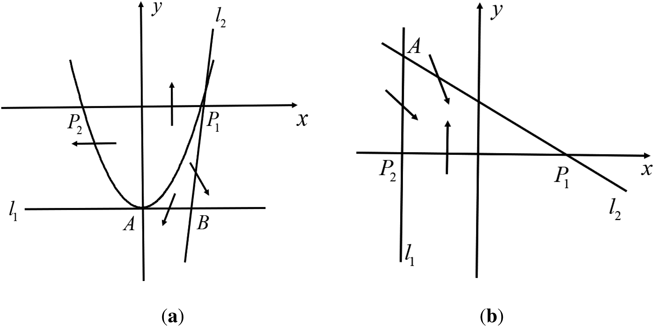
Vector field directions of system (2.3) in (x, y) phase plane. (a) Under the conditions of Theorem 2(i). (b) Under the conditions of Theorem 2 (ii).

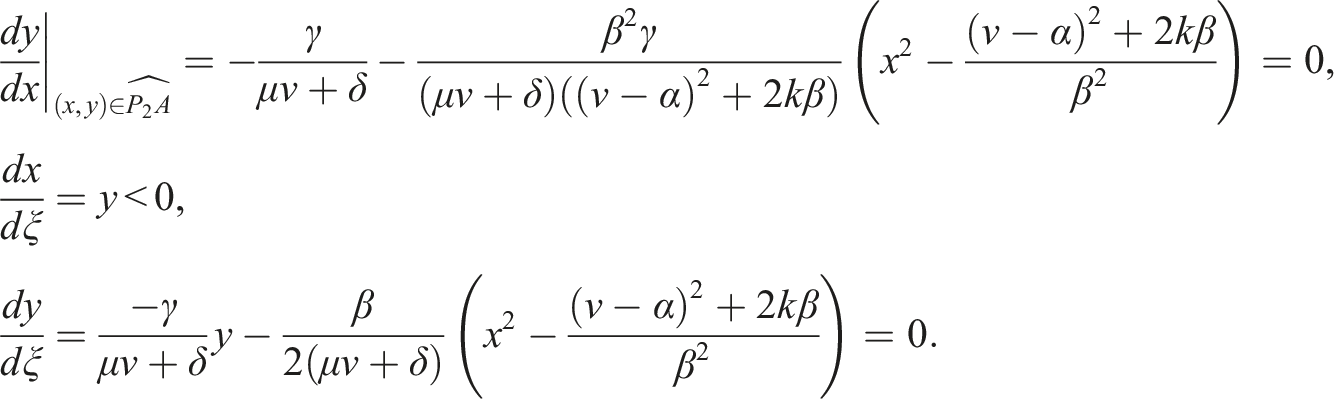
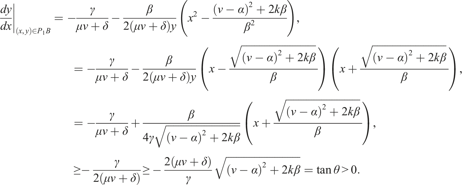
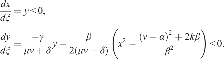
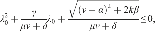
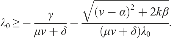
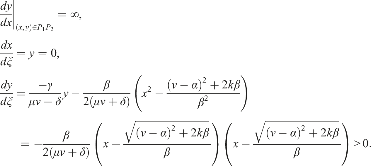
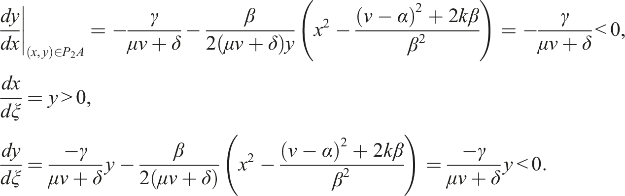
(ii) Similarly, we merely need to demonstrate that the heteroclinic orbit L (P₁, P₂) does not intersect the x-axis at any point other than P₁ and P₂. Given the conditions of Theorem 2 (ii), the characteristic equation of planar dynamical system (2.3) at P₁ (x₁, 0)

$\begin{array}{c}\hfill {\lambda }^2+\frac{\gamma }{\mu v+\delta }\lambda +\frac{\sqrt{{(v-\alpha )}^2+2k\beta }}{\mu v+\delta }=0,\hfill \end{array}$

has two different real roots

$\begin{array}{l}\hfill {\lambda }_1=\frac{-\gamma +\sqrt{{\gamma }^2-4\sqrt{{(v-\alpha )}^2+2k\beta }(\mu v+\delta )}}{2(\mu v+\delta )},\\ \hfill {\lambda }_2=\frac{-\gamma -\sqrt{{\gamma }^2-4\sqrt{{(v-\alpha )}^2+2k\beta }(\mu v+\delta )}}{2(\mu v+\delta )}.\end{array}$

Thus, there is λ₀ ∈ [λ₂, λ₁], λ₀ < 0, so that

$\begin{array}{c}\hfill {\lambda }_0^2+\frac{\gamma }{\mu v+\delta }{\lambda }_0+\frac{\sqrt{{(v-\alpha )}^2+2k\beta }}{\mu v+\delta }\le 0,\hfill \end{array}$

namely

$\begin{array}{c}\hfill {\lambda }_0\ge -\frac{\gamma }{\mu v+\delta }-\frac{\sqrt{{(v-\alpha )}^2+2k\beta }}{(\mu v+\delta ){\lambda }_0}.\hfill \end{array}$

set

$\begin{array}{c}\hfill l_1:x=-\frac{\sqrt{{(v-\alpha )}^2+2k\beta }}{\beta },l_2:y={\lambda }_0\left(x-\frac{\sqrt{{(v-\alpha )}^2+2k\beta }}{\beta }\right).\hfill \end{array}$

Then the straight lines l₁, l₂ and x-axis enclose a triangular region AP₁P₂ in Figure 2(b). The closed curve made up of the line segments AP₁, P₁P₂, and P₂A is non-tangential in general. When system (2.3) is replaced into the coordinate values of points on the line segment AP₁, P₁P₂, and P₂A yields

$\begin{array}{ll}\hfill & \frac{dy}{dx}{|}_{(x,y)\in A{P}_1}=-\frac{\gamma }{\mu v+\delta }-\frac{\beta }{2(\mu v+\delta )y}\left(x^2-\frac{{(v-\alpha )}^2+2k\beta }{{\beta }^2}\right)\hfill \\ \hfill & =-\frac{\gamma }{\mu v+\delta }-\frac{\beta }{2(\mu v+\delta ){\lambda }_0}\left(x+\frac{\sqrt{{(v-\alpha )}^2+2k\beta }}{\beta }\right)\hfill \\ \hfill & \le -\frac{\gamma }{\mu v+\delta }-\frac{\sqrt{{(v-\alpha )}^2+2k\beta }}{(\mu v+\delta ){\lambda }_0}\le {\lambda }_0<0,\hfill \\ \hfill & \frac{dx}{d\xi }=y>0,\hfill \\ \hfill & \frac{dy}{d\xi }=\frac{-\gamma }{\mu v+\delta }y-\frac{\beta }{2(\mu v+\delta )}\left(x^2-\frac{{(v-\alpha )}^2+2k\beta }{{\beta }^2}\right)\hfill \\ \hfill & =\left(x-\frac{\sqrt{{(v-\alpha )}^2+2k\beta }}{\beta }\right)\left(\frac{-\gamma }{\mu v+\delta }{\lambda }_0-\frac{\beta }{2(\mu v+\delta )}\left(x+\frac{\sqrt{{(v-\alpha )}^2+2k\beta }}{\beta }\right)\right)\hfill \\ \hfill & \le \left(x-\frac{\sqrt{{(v-\alpha )}^2+2k\beta }}{\beta }\right)\left(\frac{-\gamma }{\mu v+\delta }{\lambda }_0-\frac{\sqrt{{(v-\alpha )}^2+2k\beta }}{\mu v+\delta }\right)<0.\hfill \end{array}$

On the line segment P₁P₂

$\begin{array}{ll}\hfill & \frac{dy}{dx}{|}_{(x,y)\in P_1{P}_2}=\infty ,\hfill \\ \hfill & \frac{dx}{d\xi }=y=0,\hfill \\ \hfill & \frac{dy}{d\xi }=\frac{-\gamma }{\mu v+\delta }y-\frac{\beta }{2(\mu v+\delta )}\left(x^2-\frac{{(v-\alpha )}^2+2k\beta }{{\beta }^2}\right)\hfill \\ \hfill & =-\frac{\beta }{2(\mu v+\delta )}\left(x+\frac{\sqrt{{(v-\alpha )}^2+2k\beta }}{\beta }\right)\left(x-\frac{\sqrt{{(v-\alpha )}^2+2k\beta }}{\beta }\right)>0.\hfill \end{array}$

On the line segment P₂A

$\begin{array}{ll}\hfill & \frac{dy}{dx}{|}_{(x,y)\in P_{2}A}=-\frac{\gamma }{\mu v+\delta }-\frac{\beta }{2(\mu v+\delta )y}\left(x^2-\frac{{(v-\alpha )}^2+2k\beta }{{\beta }^2}\right)=-\frac{\gamma }{\mu v+\delta }<0,\hfill \\ \hfill & \frac{dx}{d\xi }=y>0,\hfill \\ \hfill & \frac{dy}{d\xi }=\frac{-\gamma }{\mu v+\delta }y-\frac{\beta }{2(\mu v+\delta )}\left(x^2-\frac{{(v-\alpha )}^2+2k\beta }{{\beta }^2}\right)=\frac{-\gamma }{\mu v+\delta }y<0.\hfill \end{array}$

Figure 2(b) shows the tangent slope of the orbits of system (2.3) through line segments AP₁, P₁P₂, and P₂A. The closed curve is non-tangential due to the presence of line segments AP₁, P₁P₂, and P₂A. Thus, we can infer that the heteroclinic orbit L (P₂, P₁) cannot pass through the region P₁AP₂. Furthermore, the heteroclinic orbit L (P₂, P₁) does not present another intersection point with the x-axis besides P₁ and P₂. Consequently, we explain U(ξ) has monotonically increasing property with the condition of Theorem 2 (ii). And then the monotonically increasing property of u(ξ) can be obtained and formula (3.2) holds.

Theorem 3

The hypothesis that the wave speed v and integral constant k satisfy (v − α)² + 2kβ > 0.

(i) If $-2\sqrt[4]{({(v-\alpha )}^2+2k\beta )\mathrm{\Delta }}<\gamma <0$ , Δ = (μv + δ)², after that (1.1) exists an unparalleled oscillatory damped traveling wave solution corresponding to heteroclinic orbit L (P₁, P₂) in Figure 1(d). The solution exits monotonically decreasing property at the right-hand side of $\widehat{{\xi }_1}$ , and possesses oscillatory damped property at the left-hand side of $\widehat{{\xi }_1}$ . That is to say, there is numerably infinite maximum points $\widehat{{\xi }_i}$ , i = 1, 2, …, + ∞ and minimum points $\check{{\xi }_i}$ , i = 1, 2, …, + ∞ on the ξ-axis, so as to

$\left\{\begin{array}{cc}\hfill & -\infty <\cdots <\check{{\xi }_n}<\widehat{{\xi }_n}<\cdots <\check{{\xi }_1}<\widehat{{\xi }_1}<+\infty ,\hfill \\ \hfill & {\lim }_{n\to \infty }\check{{\xi }_n}={\lim }_{n\to \infty }\widehat{{\xi }_n}=-\infty ,\hfill \end{array}\right.$

(3.6)

$\left\{\begin{array}{cc}\hfill & u(+\infty )<u(\check{{\xi }_1})<\cdots <u(\check{{\xi }_n})<\cdots <u(-\infty )<\cdots <u(\widehat{{\xi }_n})<\cdots <u(\widehat{{\xi }_1}),\hfill \\ \hfill & {\lim }_{n\to \infty }u(\check{{\xi }_n})={\lim }_{n\to \infty }u(\widehat{{\xi }_n})=u(-\infty ),\hfill \end{array}\right.$

(3.7)

$\begin{array}{c}\hfill {\lim }_{n\to \infty }(\check{{\xi }_n}-{\check{\xi }}_{n+1})={\lim }_{n\to \infty }(\widehat{{\xi }_n}-{\widehat{\xi }}_{n+1})=\frac{4\pi (\mu v+\delta )}{\sqrt{4\sqrt{{(v-\alpha )}^2+2k\beta }(\mu v+\delta )-{\gamma }^2}}.\hfill \end{array}$

(3.8)

(ii) If $0<\gamma <2\sqrt[4]{({(v-\alpha )}^2+2k\beta )\mathrm{\Delta }}$ , Δ = (μv + δ)², after that (1.1) possesses an unparalleled oscillatory damped traveling wave solution corresponding to heteroclinic orbit L (P₂, P₁) in Figure 1(c). The solution exits monotonically increasing property at the left-hand side of $\check{{\xi }_1}$ , and possesses oscillatory damped property at the right-hand side of $\check{{\xi }_1}$ . That is to say, there is numerably infinite maximum points $\check{{\xi }_i}$ , i = 1, 2, …, + ∞ and minimum points $\widehat{{\xi }_i}$ , i = 1, 2, …, + ∞ on the ξ-axis, so as to

$\left\{\begin{array}{cc}\hfill & -\infty <\widehat{{\xi }_1}<\check{{\xi }_1}<\cdots <\widehat{{\xi }_n}<\check{{\xi }_n}<+\infty ,\hfill \\ \hfill & {\lim }_{n\to \infty }\check{{\xi }_n}={\lim }_{n\to \infty }\widehat{{\xi }_n}=+\infty ,\hfill \end{array}\right.$

(3.9)

$\left\{\begin{array}{cc}\hfill & u(-\infty )<u(\check{{\xi }_1})<\cdots <u(\check{{\xi }_n})<\cdots <u(+\infty )<\cdots <u(\widehat{{\xi }_n})<\cdots <u(\widehat{{\xi }_1}),\hfill \\ \hfill & {\lim }_{n\to \infty }u(\check{{\xi }_n})={\lim }_{n\to \infty }u(\widehat{{\xi }_n})=u(+\infty ),\hfill \end{array}\right.$

(3.10)

$\begin{array}{c}\hfill {\lim }_{n\to \infty }(\check{{\xi }_n}-{\check{\xi }}_{n+1})={\lim }_{n\to \infty }(\widehat{{\xi }_n}-{\widehat{\xi }}_{n+1})=\frac{4\pi (\mu v+\delta )}{\sqrt{4\sqrt{{(v-\alpha )}^2+2k\beta }(\mu v+\delta )-{\gamma }^2}}.\hfill \end{array}$

(3.11)

Proof

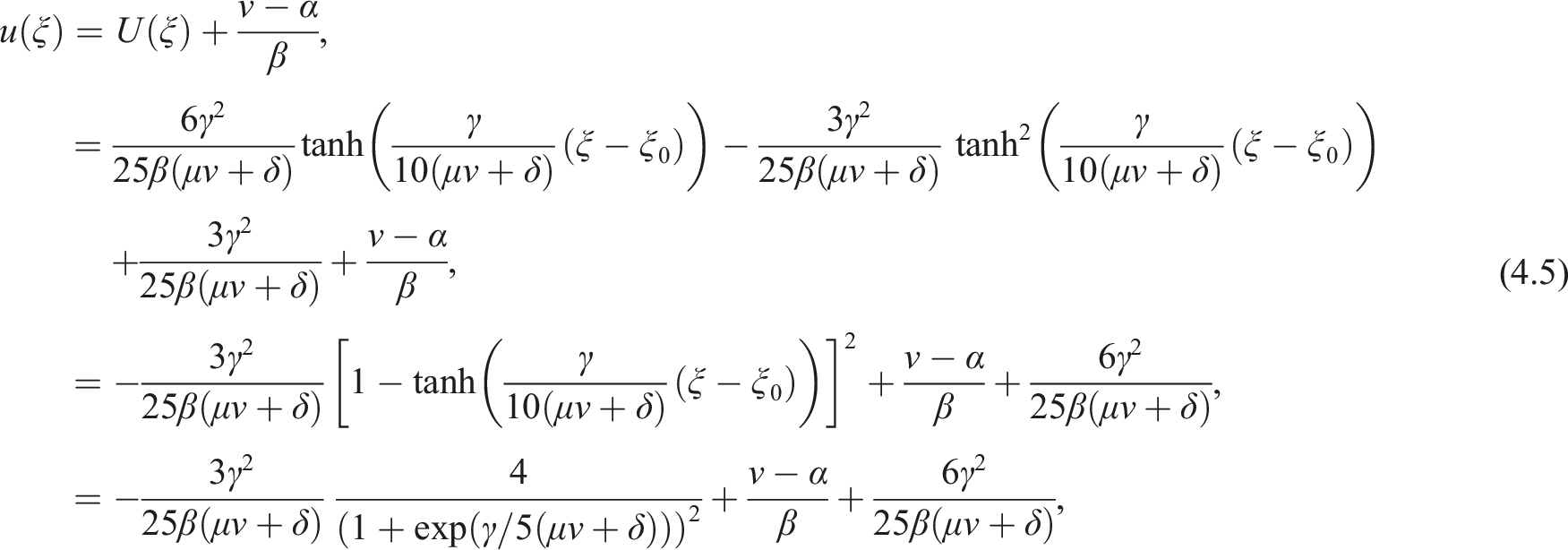
We mainly prove that (i) holds. Owing to the fact that the bounded traveling wave solutions u(ξ) of (1.1) and U(ξ) of (2.2) meet u(ξ) = U(ξ) + v − α/β, it is possible to derive the characteristics of the bounded traveling wave solutions u(ξ) of equation (1.1) by investigating the characteristics of the solution U(ξ) of equation (2.2). Based on the consideration in previous section, obviously, P₁ and P₂ are severally an unstable focus point and a saddle point under the condition of Theorem 3(i). Moreover, the orbit L(P₁, P₂) tends to P₁ spirally as ξ tends to −∞. The intersection points of the orbit L(P₁, P₂) and x-axis at the right-hand side of P₁ corresponding to maximum points of U(ξ), while the ones at the left-hand side of P₁ corresponding to minimum points of U(ξ). Consequently, on the basis of the relationship between the equations (1.1) and (2.2), the equations (3.6), (3.7) hold. In addition, as L(P₁, P₂) tends to P₁ sufficiently, its property is close to the property of the linear approximate solution of system (2.3). Thus, the frequency of the orbit rotating around P₁ tends to $\sqrt{4\sqrt{{(v-\alpha )}^2+2k\beta }(\mu v+\delta )-{\gamma }^2}/4\pi (\mu v+\delta )$ . Furthermore, (3.8) holds from the relationship between equations (1.1) and (2.2). Assertion

(ii) could be explained similarly.

Due to the shape and speed of the traveling wave solution stay the same as parallel along the ξ-axis, therefore, we can choose $\widehat{{\xi }_1}=0$ , after that the oscillatory damped solution investigated in Theorem 3 is depicted in Figure 3.

Figure 3.

(Color online) Oscillatory damped solution. (a) Corresponding to L (P2, P1) in Figure 1(e), (b) Corresponding to L (P1, P2) in Figure 1(d).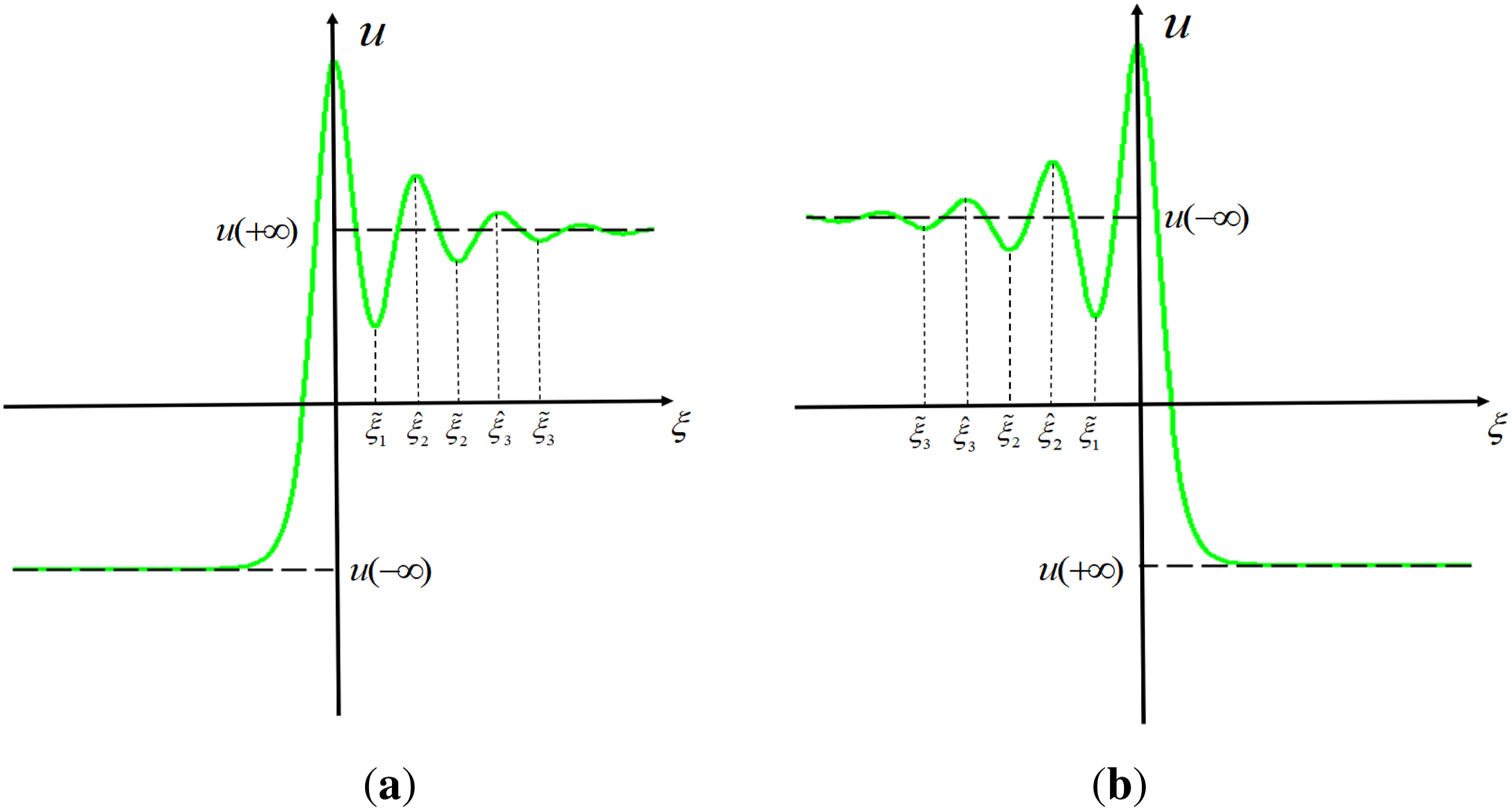

Solitary wave and approximate oscillatory damped solutions

Bell profile solitary wave solution and kink profile solitary wave solution

It is evident follow the preceding explanation that equation (1.1) exhibits a bell profile solitary wave solution as γ = 0. Additionally, the equation (1.1) also admits a kink profile solitary wave solution whenγ ≠ 0. Both the bell profile solitary wave solution of equation (1.1) and the kink profile solitary wave solution satisfying formula (2.2), according to Refs. 54 and 55, with the help of undetermined coefficients method, let’s assume that solutions of the equation (2.2) is

$\begin{array}{c}\hfill U(\xi )=a_0+a_1\tanh \left(\omega (\xi -{\xi }_0)\right)+a_2{\tanh }^2\left(\omega (\xi -{\xi }_0)\right).\hfill \end{array}$

(4.1)

In the formula, a₀, a₁, a₂, ω are confirmed coefficients, ξ₀ is an arbitrary real number. By substituting equation (4.1) into equation (2.2), through some simple calculations and reductions, we obtain that a₀, a₁, a₂, and ω are satisfied.

$\left\{\begin{array}{cc}\hfill & 12\beta \mu \nu {\omega }^2{a}_2+12\beta \delta {\omega }^2{a}_2+{\beta }^2{a}_2^2=0,\hfill \\ \hfill & 4\beta \mu \nu {\omega }^2{a}_1+4\beta \delta {\omega }^2{a}_1+2{\beta }^2{a}_1{a}_2-4\beta \gamma \omega a_2=0,\hfill \\ \hfill & -16\beta \mu \nu {\omega }^2{a}_2-16\beta \delta {\omega }^2{a}_2+2{\beta }^2{a}_0{a}_2+{\beta }^2{a}_1^2-2\beta \gamma \omega a_1=0,\hfill \\ \hfill & -4\beta \mu \nu {\omega }^2{a}_1-4\beta \delta {\omega }^2{a}_1+2{\beta }^2{a}_0{a}_1+4\beta \gamma \omega a_2=0,\hfill \\ \hfill & 4\beta \mu \nu {\omega }^2{a}_2+4\beta \delta {\omega }^2{a}_2+{\beta }^2{a}_0{a}_0+2\beta \gamma \omega a_1-{\alpha }^2+2\alpha \nu -2\beta k-{\nu }^2=0.\hfill \end{array}\right.$

(4.2)

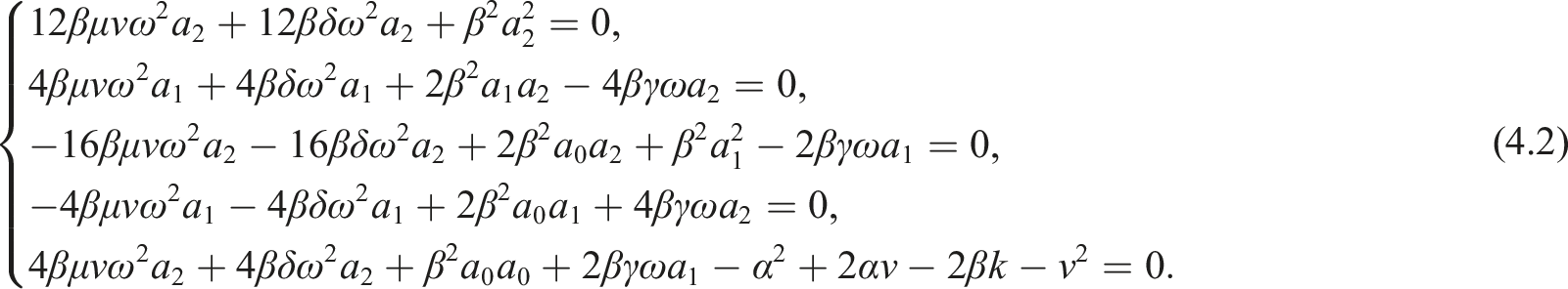
Solving equation (4.2) for γ = 0 and γ ≠ 0, and taking the results into (4.1) yields the following assertion.

Theorem 4

The hypothesis that wave speed v and integral constant k meet (v − α)² + 2kβ > 0,

(i) If γ = 0, then Equation. (2.2) exists a bell profile solitary wave solution in the following form

$\begin{array}{ll}\hfill & U(\xi )=\frac{2\sqrt{{(v-\alpha )}^2+2k\beta }}{\beta }-\frac{3\sqrt{{(v-\alpha )}^2+2k\beta }}{\beta }{\tanh }^2\left(\frac{\sqrt[4]{{(v-\alpha )}^2+2k\beta }}{2\sqrt{\mu \nu +\delta }}(\xi -{\xi }_0)\right),\hfill \\ \hfill & =\frac{3\sqrt{{(v-\alpha )}^2+2k\beta }}{\beta }sec{h}^2\left(\frac{\sqrt[4]{{(v-\alpha )}^2+2k\beta }}{2\sqrt{\mu \nu +\delta }}(\xi -{\xi }_0)\right)-\frac{\sqrt{{(v-\alpha )}^2+2k\beta }}{\beta },\hfill \end{array}$

(4.3)

and then the equation (1.1) possesses a bell profile solitary wave solution in the following form

$\begin{array}{c}\hfill u(\xi )=U(\xi )+\frac{v-\alpha }{\beta }.\hfill \end{array}$

(4.4)

(ii) Suppose that the dissipation coefficient γ and the wave speed v meet $\sqrt{{(v-\alpha )}^2+2k\beta }=6{\gamma }^2/25(\mu \nu +\delta )$ , then Equation. (2.2) possesses a monotone kink profile solitary wave solution

$\begin{array}{ll}\hfill & u(\xi )=U(\xi )+\frac{v-\alpha }{\beta },\hfill \\ \hfill & =\frac{6{\gamma }^2}{25\beta (\mu \nu +\delta )}\tanh \left(\frac{\gamma }{10(\mu \nu +\delta )}(\xi -{\xi }_0)\right)-\frac{3{\gamma }^2}{25\beta (\mu \nu +\delta )}{\tanh }^2\left(\frac{\gamma }{10(\mu \nu +\delta )}(\xi -{\xi }_0)\right)\hfill \\ \hfill & +\frac{3{\gamma }^2}{25\beta (\mu \nu +\delta )}+\frac{v-\alpha }{\beta },\hfill \\ \hfill & =-\frac{3{\gamma }^2}{25\beta (\mu \nu +\delta )}{\left[1-\tanh \left(\frac{\gamma }{10(\mu \nu +\delta )}(\xi -{\xi }_0)\right)\right]}^2+\frac{v-\alpha }{\beta }+\frac{6{\gamma }^2}{25\beta (\mu \nu +\delta )},\hfill \\ \hfill & =-\frac{3{\gamma }^2}{25\beta (\mu \nu +\delta )}\frac{4}{{\left(1+\exp (\gamma /5(\mu \nu +\delta ))\right)}^2}+\frac{v-\alpha }{\beta }+\frac{6{\gamma }^2}{25\beta (\mu \nu +\delta )},\hfill \end{array}$

(4.5)

and then the Equation (1.1) exists a kink profile solitary wave solution in the following form

$\begin{array}{c}\hfill u(\xi )=U(\xi )+\frac{v-\alpha }{\beta }.\hfill \end{array}$

(4.6)

Proof

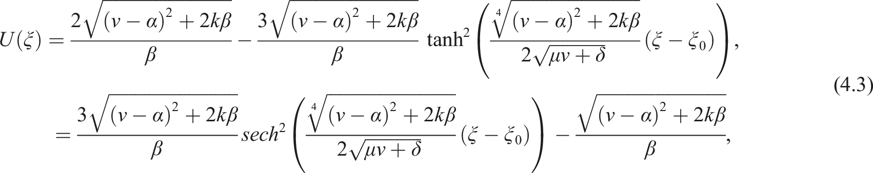
Considering claim (i), if γ = 0, then solving equation (4.2), we obtain

$\begin{array}{c}\hfill a_0=\frac{2\sqrt{{(v-\alpha )}^2+2k\beta }}{\beta },a_1=0,a_2=-\frac{3\sqrt{{(v-\alpha )}^2+2k\beta }}{\beta },\omega =\frac{\sqrt[4]{{(v-\alpha )}^2+2k\beta }}{2\sqrt{\mu \nu +\delta }}.\hfill \end{array}$

(4.7)

It is substituted into formula (4.1), and the results are rearranged to obtain the bell profile solitary wave solution U(ξ) which is consistent with L (P₂, P₂) in Figure 1(a).

After that we certificate deduction (ii). Assuming that $\sqrt{{(v-\alpha )}^2+2k\beta }=6{\gamma }^2/25(\mu \nu +\delta )$ , the dissipation coefficient γ and the wave speed v meet the condition of Assertion 2. So, it is obtained by solving Eq. (4.2)

$\begin{array}{c}\hfill a_0=\frac{3{\gamma }^2}{25\beta (\mu \nu +\delta )},a_1=\frac{6{\gamma }^2}{25\beta (\mu \nu +\delta )},a_2=-\frac{3{\gamma }^2}{25\beta (\mu \nu +\delta )},\omega =\frac{\gamma }{10(\mu \nu +\delta )}.\hfill \end{array}$

(4.8)

Taking it into (4.1) yields the kink profile solitary wave solution U(ξ) which is consistent with L (P₁, P₂) in Figure 1(b) (γ(μv + δ) < 0) or L (P₂, P₁) in Figure 1(e) (γ(μv + δ) > 0).

Approximate oscillatory damped solutions

According to assertion 3, as the dissipation coefficient γ as well as the wave velocity v meet $0<|\gamma /\mu \nu +\delta |<2\sqrt[4]{{(v-\alpha )}^2+2k\beta }$ , equation (1.1) exists oscillatory damped solutions. Due to its exact expression is difficult to get, we are going to present its approximate oscillatory damped solutions of the equation (1.1). It follows from the theory of planar dynamical systems that the heteroclinic orbit L (P₂, P₁) in Figure 1(c) results in the break of homoclinic orbit L (P₂, P₂) in Figure 1(a) under the effect of dissipation coefficient γ. Therefore, the non-oscillatory part of the oscillatory damped solution which is consistent with the heteroclinic orbit L (P₂, P₁) in Figure 1(c) can be expressed as equation (4.4)

$\begin{array}{ll}\hfill & u_1(\xi )=\frac{3\sqrt{{(v-\alpha )}^2+2k\beta }}{\beta }sec{h}^2\left(\frac{\sqrt[4]{{(v-\alpha )}^2+2k\beta }}{2\sqrt{\mu \nu +\delta }}(\xi -{\xi }_0)\right)+\frac{v-\alpha -\sqrt{{(v-\alpha )}^2+2k\beta }}{\beta },\hfill \\ \hfill & \xi \in (-\infty ,{\xi }_0].\hfill \end{array}$

(4.9)

however, the oscillatory part of the oscillatory damped solution can be approximated as following

$\begin{array}{c}\hfill u_2(\xi )=\exp (r(\xi -{\xi }_0))\left[A_1\cos (B(\xi -{\xi }_0))-A_2\sin (B(\xi -{\xi }_0))\right]+C,\hfill \end{array}$

(4.10)

where A₁, A₂, B, C, and r are all undetermined coefficients. The equation (4.10) exists both damped and oscillatory property, in which $e^{r(\xi -{\xi }_0)}$ possesses damped property and A₁ cos (B (ξ − ξ₀)) − A₂ sin (B (ξ − ξ₀)) has oscillatory property. It can be obtained by plugging (4.10) into (2.1) and removing the term containing $e^{2r(\xi -{\xi }_0)}$

$\begin{array}{c}\hfill B^2=\frac{-{\gamma }^2+4C\beta (\mu \nu +\delta )-4(v-\alpha )(\mu \nu +\delta )}{4{(\mu \nu +\delta )}^2},r=\frac{-\gamma }{2(\mu \nu +\delta )},k=C(v-\alpha )+\frac{C^2\beta }{2}.\hfill \end{array}$

(4.11)

To investigate the approximate oscillatory damped solution of the equation (1.1), certain conditions are required to connect the non-oscillatory part u₁(ξ) to the oscillatory part u₂(ξ), ξ₀ = 0 is taken as the contact point due to the waveform of the solution remain unchanged with translation along ξ-axis. So we choose

$\begin{array}{c}\hfill \frac{d^i}{d{\xi }^i}{u}_2(0)=\frac{d^i}{d{\xi }^i}{u}_1(0),i=\mathrm{0,1}.\hfill \end{array}$

(4.12)

It can be known that from (4.12)

$\begin{array}{c}\hfill A_1+C=u_1(0),A_{1}r-A_{2}B=0.\hfill \end{array}$

(4.13)

When ξ approaches +∞, equation (4.10) approaches C. Paying attention to that (4.10) in accordance with the oscillatory part of the oscillatory damped solution and that the heteroclinic orbit L (P₂, P₁) tends to (D₁, 0) as ξ → +∞. As a result, we get

$\begin{array}{c}\hfill C=D_1=\frac{v-\alpha }{\beta }+x_1,B^2=\frac{4(\mu \nu +\delta )\sqrt{{(v-\alpha )}^2+2k\beta }-{\gamma }^2}{4{(\mu \nu +\delta )}^2}.\hfill \end{array}$

(4.14)

The value of A₁ cos (B (ξ − ξ₀)) − A₂ sin (B (ξ − ξ₀)) + C has nothing to do with the value of B. So, it can be assumed that B > 0, according to (4.13), we can obtain

$\begin{array}{c}\hfill A_1=\frac{\sqrt{{(v-\alpha )}^2+2k\beta }}{\beta }=x_1,A_2=-\frac{\gamma \sqrt{{(v-\alpha )}^2+2k\beta }}{\beta \sqrt{4(\mu \nu +\delta )\sqrt{{(v-\alpha )}^2+2k\beta }-{\gamma }^2}}.\hfill \end{array}$

(4.15)

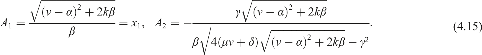
Then, we get the following theorem.

Theorem 5

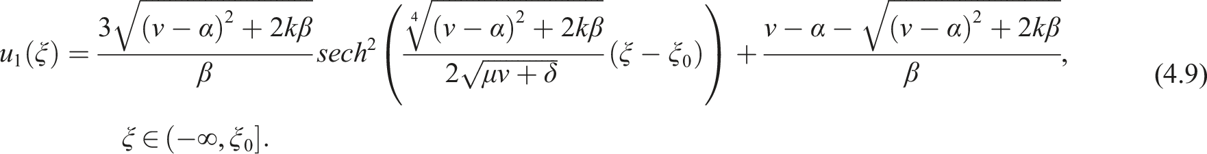
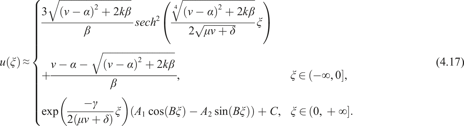
Assume wave speed v and integral constant k fulfill the inequality (v − α)² + 2kβ > 0. (i) The hypothesis that v and dissipation coefficient γ meet $-2\sqrt[4]{I}f({(v-\alpha )}^2+2k\beta )\mathrm{\Delta }<\gamma <0$ and Δ = (μv + δ)², then the Equation (1.1) exists an oscillatory damped solution corresponding to the heteroclinic orbit L(P₁, P₂) in Figure 1(d), its approximate solution is

$u(\xi )\approx \left\{\begin{array}{cc}\hfill & \frac{3\sqrt{{(v-\alpha )}^2+2k\beta }}{\beta }sec{h}^2\left(\frac{\sqrt[4]{{(v-\alpha )}^2+2k\beta }}{2\sqrt{\mu \nu +\delta }}\xi \right)\hfill \\ \hfill & +\frac{v-\alpha -\sqrt{{(v-\alpha )}^2+2k\beta }}{\beta },\xi \in (0,+\infty ],\hfill \\ \hfill & \exp \left(\frac{-\gamma }{2(\mu \nu +\delta )}\xi \right)\left(A_1\cos (B\xi )-A_2\sin (B\xi )\right)+C,\xi \in (-\infty ,0].\hfill \end{array}\right.$

(4.16)

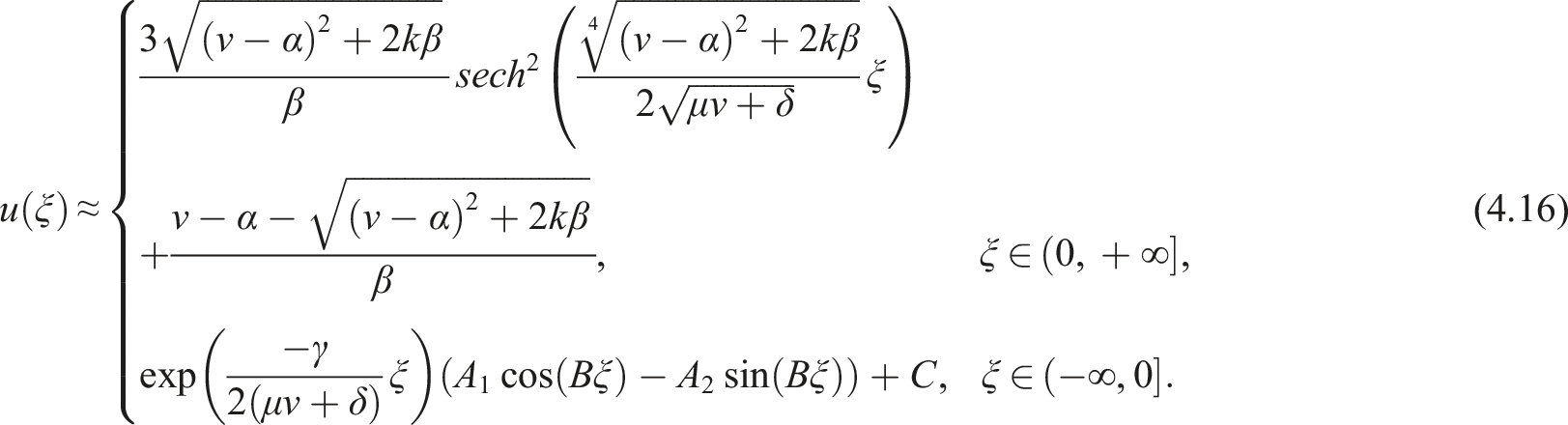
(ii) The hypothesis that v and the dissipation coefficient γ meet $0<\gamma <2\sqrt[4]{({(v-\alpha )}^2+2k\beta )\mathrm{\Delta }}$ , Δ = (μv + δ)², then the Equation (1.1) possesses an oscillatory damped solution in accordance with the heteroclinic orbit L (P₂, P₁) in Figure 1(c), its approximate solution is

$u(\xi )\approx \left\{\begin{array}{cc}\hfill & \frac{3\sqrt{{(v-\alpha )}^2+2k\beta }}{\beta }sec{h}^2\left(\frac{\sqrt[4]{{(v-\alpha )}^2+2k\beta }}{2\sqrt{\mu \nu +\delta }}\xi \right)\hfill \\ \hfill & +\frac{v-\alpha -\sqrt{{(v-\alpha )}^2+2k\beta }}{\beta },\xi \in (-\infty ,0],\hfill \\ \hfill & \exp \left(\frac{-\gamma }{2(\mu \nu +\delta )}\xi \right)\left(A_1\cos (B\xi )-A_2\sin (B\xi )\right)+C,\xi \in (0,+\infty ].\hfill \end{array}\right.$

(4.17)

where A₁, A₂, B, and C in Equations (4.16) and (4.17) are confirmed through Equations. (4.14) and (4.15).

Error estimates for approximate oscillatory damped solutions

In this section, in order to investigate errors between exact oscillatory damped solution in accordance with L (P₂, P₁) and approximate oscillatory damped solutions (4.17), we take Figure 1(c) as an example.

Assuming that D₁ = v − α/β + x₁, D₂ = v − α/β + x₂, then substituting

$\begin{array}{c}\hfill W(\xi )=\frac{u(\xi )-D_1}{D_2-D_1},\hfill \end{array}$

(5.1)

into the equation (2.1), it is obvious that the exact oscillatory damped solutions of (2.1) can be reduced to the following initial value problem

$\begin{array}{ll}\hfill & W_{\xi \xi }^{\prime \prime }(\xi )+\frac{\gamma }{\mu \nu +\delta }{W}_{\xi }^{\prime }(\xi )+\frac{\sqrt{{(v-\alpha )}^2+2k\beta }}{\mu \nu +\delta }W(\xi )=\frac{\sqrt{{(v-\alpha )}^2+2k\beta }}{\mu \nu +\delta }{W}^2(\xi ),\hfill \\ \hfill & W(0)=\frac{u(0)-D_1}{D_2-D_1}=-\frac{1}{2},W_{\xi }^{\prime }(0)=0,\hfill \end{array}$

(5.2)

under the initial condition

$\begin{array}{c}\hfill u(0)=\frac{v-\alpha +2\sqrt{{(v-\alpha )}^2+2k\beta }}{\beta },u^{\prime }(0)=0.\hfill \end{array}$

(5.3)

Proposition 3

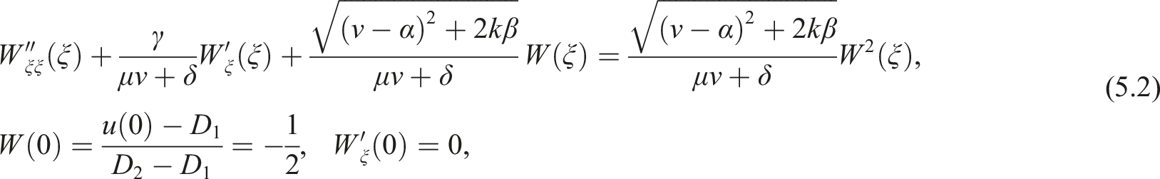
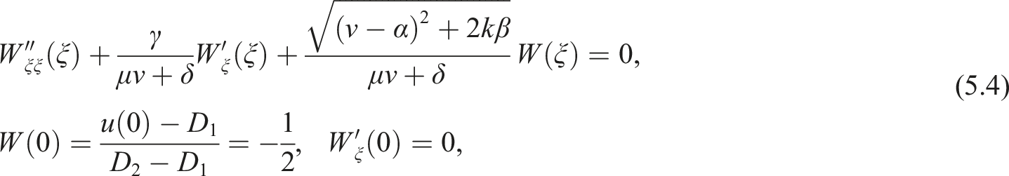
Suppose that W₁(ξ) and W₂(ξ) are solutions of

$\begin{array}{ll}\hfill & W_{\xi \xi }^{\prime \prime }(\xi )+\frac{\gamma }{\mu \nu +\delta }{W}_{\xi }^{\prime }(\xi )+\frac{\sqrt{{(v-\alpha )}^2+2k\beta }}{\mu \nu +\delta }W(\xi )=0,\hfill \\ \hfill & W(0)=\frac{u(0)-D_1}{D_2-D_1}=-\frac{1}{2},W_{\xi }^{\prime }(0)=0,\hfill \end{array}$

(5.4)

and

$\begin{array}{ll}\hfill & W_{\xi \xi }^{\prime \prime }(\xi )+\frac{\gamma }{\mu \nu +\delta }{W}_{\xi }^{\prime }(\xi )+\frac{\sqrt{{(v-\alpha )}^2+2k\beta }}{\mu \nu +\delta }W(\xi )=\frac{\sqrt{{(v-\alpha )}^2+2k\beta }}{\mu \nu +\delta }{W}^2(\xi ),\hfill \\ \hfill & W(0)=0,W_{\xi }^{\prime }(0)=0,\hfill \end{array}$

(5.5)

then W₁(ξ) + W₂(ξ) is a solution of Equation (5.2).

Proposition 4

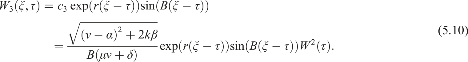
Hypothesis that W₃(ξ, τ) is a solution of

$\begin{array}{ll}\hfill & W_{\xi \xi }^{\prime \prime }(\xi )+\frac{\gamma }{\mu \nu +\delta }{W}_{\xi }^{\prime }(\xi )+\frac{\sqrt{{(v-\alpha )}^2+2k\beta }}{\mu \nu +\delta }W(\xi )=0,\hfill \\ \hfill & W(\tau )=0,W_{\xi }^{\prime }(\tau )=\frac{\sqrt{{(v-\alpha )}^2+2k\beta }}{\mu \nu +\delta }{W}^2(\tau ),\hfill \end{array}$

(5.6)

then ${\int }_0^{\xi }{W}_3(\xi ,\tau )d\tau$ is a solution of Eq. (5.5).

It is clear that the solution of (5.4) exists the following form

$\begin{array}{c}\hfill W_1(\xi )=\exp \left(c_1\cos (B\xi )+c_2\sin (B\xi )\right),\hfill \end{array}$

(5.7)

in which c₁ = − $\frac{1}{2}$ , c₂ = $\frac{r}{2B}$ with r, B being confirmed in (4.11), (4.14). With the help of variable change t = ξ − τ, (5.6) can be rewritten as

$\begin{array}{ll}\hfill & V_{tt}^{\prime \prime }(t,\tau )+\frac{\gamma }{\mu \nu +\delta }{V}_t^{\prime }(t,\tau )+\frac{\sqrt{{(v-\alpha )}^2+2k\beta }}{\mu \nu +\delta }V(t,\tau )=0,\hfill \\ \hfill & V(0,\tau )=0,V_t^{\prime }(0,\tau )=\frac{\sqrt{{(v-\alpha )}^2+2k\beta }}{\mu \nu +\delta }{W}^2(\tau ),\hfill \\ \hfill & V(t,\tau )=W_3(t+\tau ,\tau )=W_3(\xi ,\tau ).\hfill \end{array}$

(5.8)

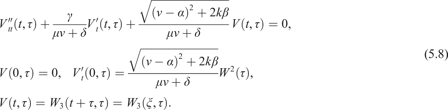
It is obvious that the solution of (5.8) has the following form

$\begin{array}{c}\hfill V(t,\tau )=c_3\exp (rt)\sin (Bt),\hfill \end{array}$

(5.9)

in which $c_3=\sqrt{{(v-\alpha )}^2+2k\beta }{W}^2(\tau )/B(\mu \nu +\delta )$ .

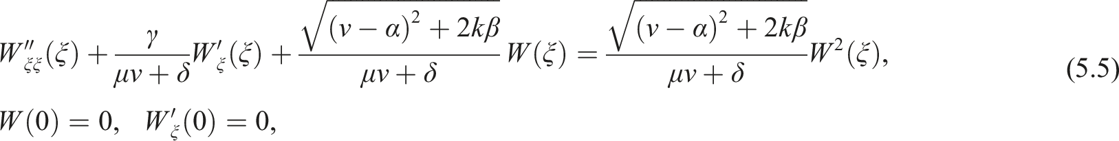
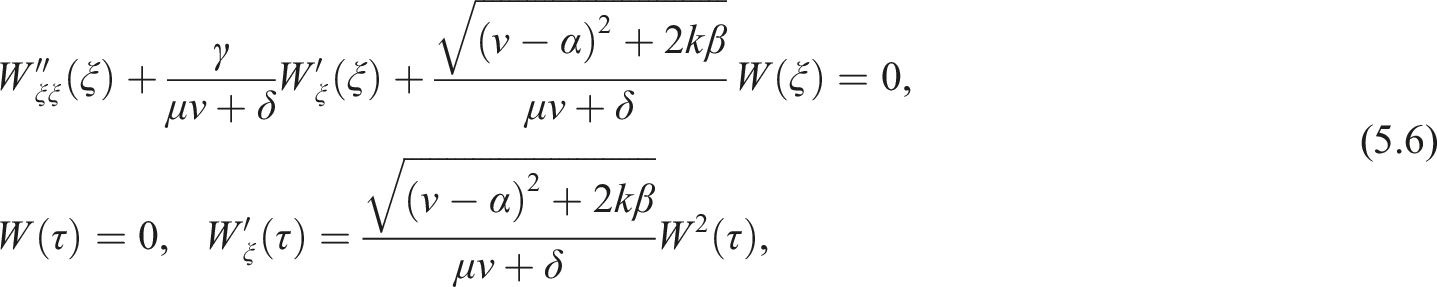
Therefore, the solution of equation (5.6) can be easily found as follows

$\begin{array}{ll}\hfill & W_3(\xi ,\tau )=c_3\exp (r(\xi -\tau ))\sin (B(\xi -\tau ))\hfill \\ \hfill & =\frac{\sqrt{{(v-\alpha )}^2+2k\beta }}{B(\mu \nu +\delta )}\exp (r(\xi -\tau ))\sin (B(\xi -\tau ))W^2(\tau ).\hfill \end{array}$

(5.10)

According to Proposition 4 and the above formula, we can derive the solution of equation (5.5)

$\begin{array}{c}\hfill W_2(\xi )={\int }_0^{\xi }{W}_3(\xi ,\tau )d\tau =\frac{\sqrt{{(v-\alpha )}^2+2k\beta }}{B(\mu \nu +\delta )}{\int }_0^{\xi }\exp (r(\xi -\tau ))\sin (B(\xi -\tau ))W^2(\tau )d\tau .\hfill \end{array}$

(5.11)

Furthermore, based on the Proposition 3, the solution of (5.2) can be easily obtained

$\begin{array}{ll}\hfill & W(\xi )=W_1(\xi )+W_2(\xi )\hfill \\ \hfill & =\exp \left(c_1\cos (B\xi )+c_2\sin (B\xi )\right)\hfill \\ \hfill & +\frac{\sqrt{{(v-\alpha )}^2+2k\beta }}{B(\mu \nu +\delta )}{\int }_0^{\xi }\exp (r(\xi -\tau ))\sin (B(\xi -\tau ))W^2(\tau )d\tau .\hfill \end{array}$

(5.12)

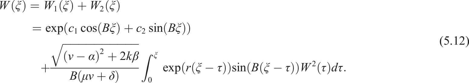
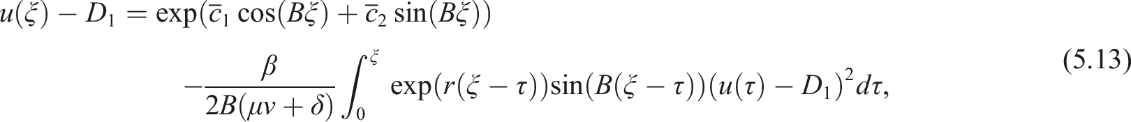
Based on (5.1) and (5.12), then the oscillatory damped solution of (1.1) satisfying the condition (5.3) that can be established

$\begin{array}{ll}\hfill & u(\xi )-D_1=\exp \left({\overline{c}}_1\cos (B\xi )+{\overline{c}}_2\sin (B\xi )\right)\hfill \\ \hfill & -\frac{\beta }{2B(\mu \nu +\delta )}{\int }_0^{\xi }\exp (r(\xi -\tau ))\sin (B(\xi -\tau )){(u(\tau )-D_1)}^{2}d\tau ,\hfill \end{array}$

(5.13)

in which ${\overline{c}}_1=x_1=A_1,{\overline{c}}_2=-A_2=-x_{1}r/B$ . As far as we know, the oscillatory damped solution is bounded, so there is a M > 0, which makes |u(ξ)| < M. Accordingly, it can be obtained from the above equation

$\begin{array}{c}\hfill |u(\xi )-D_1|\le S_1\exp (r\xi )+S_2{\int }_0^{\xi }\exp (r(\xi -\tau ))|u(\tau )-D_1|d\tau ,\xi >0,\hfill \end{array}$

(5.14)

in which

$\begin{array}{c}\hfill S_1=|{\overline{c}}_1|+|{\overline{c}}_2|,S_2=\frac{\beta }{2B(\mu \nu +\delta )}(M+|D_1|).\hfill \end{array}$

(5.15)

According to the Gronwall inequality, the above formula can be reduced to

$\begin{array}{c}\hfill |u(\xi )-D_1|\le S_3\exp (r\xi ),\xi >0,\hfill \end{array}$

(5.16)

in which S₃ = S₁ exp (S₂/r). Equations (5.16) notes that u(ξ) verges to D₁ as ξ → +∞. Finally, by connecting equation (5.13) with (5.16), it can be obtained

$\begin{array}{c}\hfill |u(\xi )-e^{-\gamma \xi /2(\mu \nu +\delta )}\left[A_1\cos (B\xi )-A_2\sin (B\xi )\right]+C|\le \frac{\beta S_3^2}{2B(\mu \nu +\delta )r}{e}^{2r\xi }(1-e^{r\xi }),\xi >0.\hfill \end{array}$

(5.17)

We can infer that the error between the exact oscillatory damped solution corresponding to L (P₂, P₁) and the approximate oscillatory damped solution equation (4.17) is less than

$\begin{array}{c}\hfill \epsilon (\xi )=\frac{\beta S_3^2}{2B(\mu \nu +\delta )r}\exp (2r\xi )(1-\exp (r\xi ))=O(\exp (2r\xi )),\xi \to +\infty .\hfill \end{array}$

(5.18)

Thus, (4.17) is significant as an approximate solution of (1.1) while the conditions in Theorem 4(i) are established. In a similar way, we can build up the integral relationship between the implicit exact damped oscillatory solution and approximate damped oscillatory solution corresponding to L (P₁, P₂) by the virtue of constant variation method.

We take γ = 0.5, 1, 2, as shown in Figures 4–6. To explain the effect of dissipation coefficient γ about oscillatory damped solution, the following parameter values are taken to satisfy the condition of Theorem 5(i) as v = 3, α = 1, k = −1/2, β = 3, μ = 1/3, δ = 1. Meanwhile, the critical value in Theorem 5(i) is $2\sqrt{2}$ . Based on Theorem 5(i), if the dissipation coefficient γ meets $0<\gamma <2\sqrt{2}$ , then the equation (1.1) exists oscillatory damped solutions.

Figure 4.

(Color online) Approximate oscillatory damped solution of the equation (1.1) with γ = 0.5.

Figure 5.

(Color online) Approximate oscillatory damped solution of the equation (1.1) with γ = 1.

Figure 6.

(Color online) Approximate oscillatory damped solution of the equation (1.1) with γ = 2.

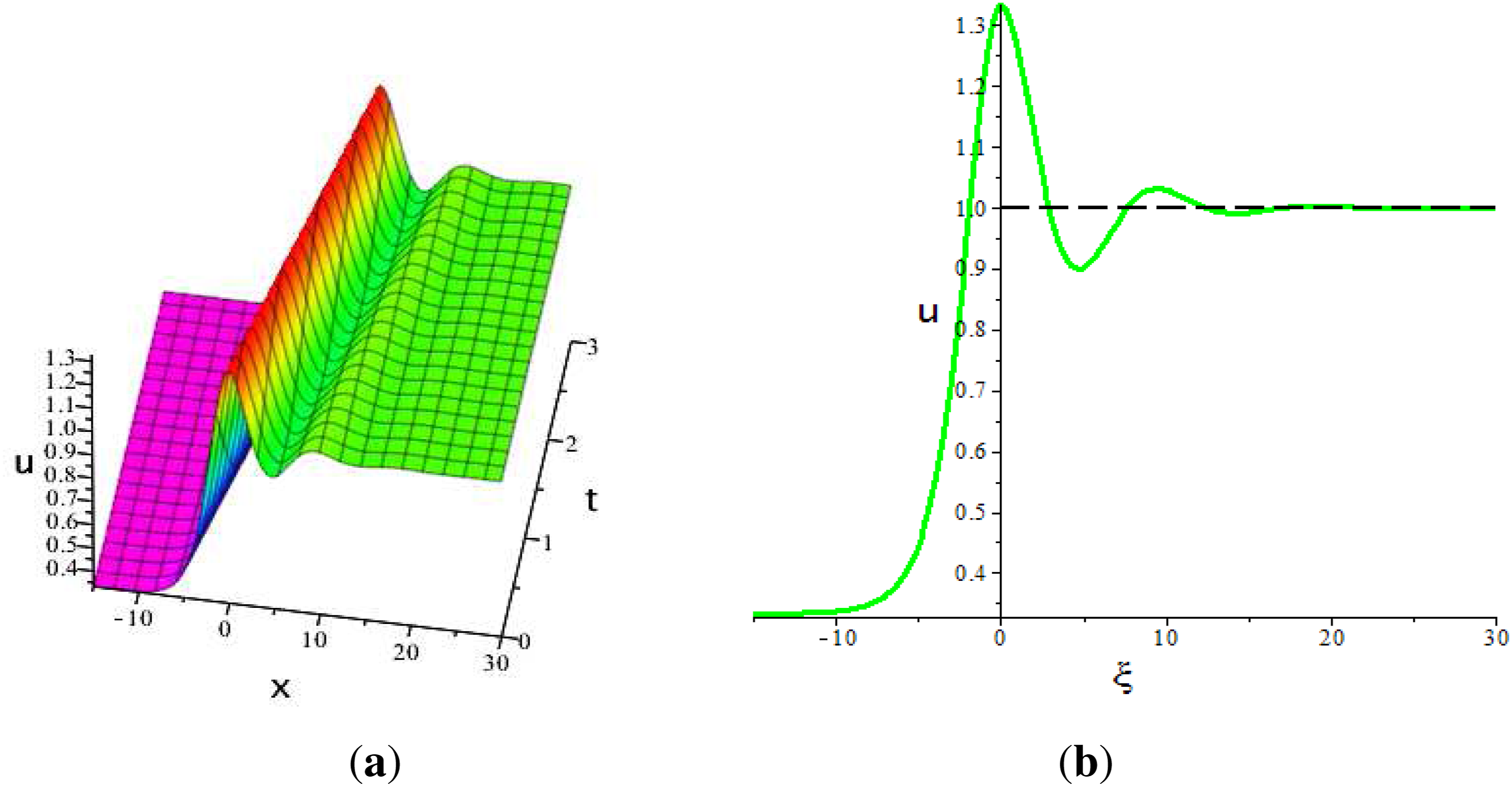
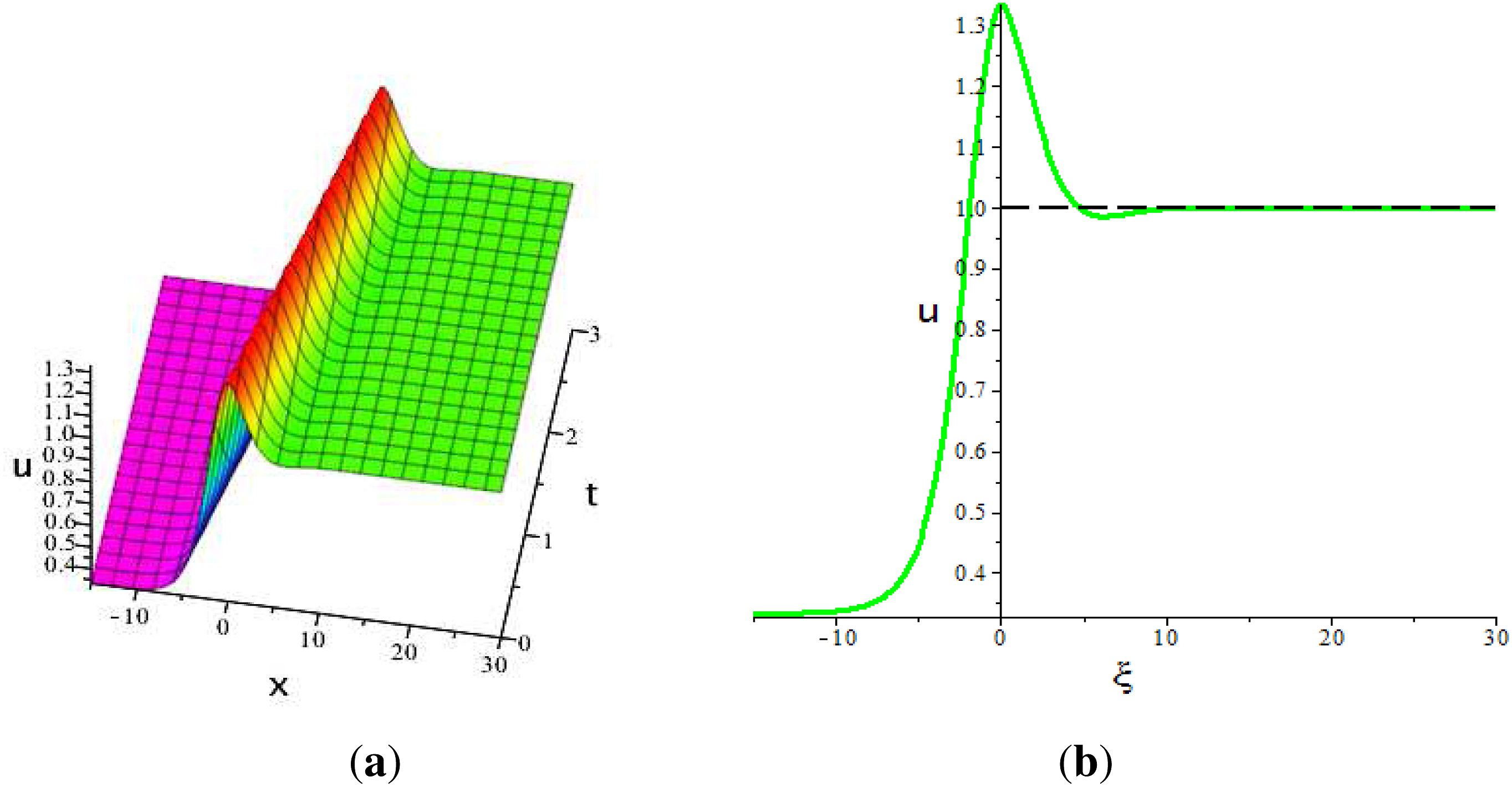
When $0<\gamma <2\sqrt[4]{({(v-\alpha )}^2+2k\beta )\mathrm{\Delta }}$ , Δ = (μv + δ)², the oscillatory damped solutions of the equation (1.1) on (0, + ∞) are able to be denoted by

$\begin{array}{ll}\hfill u(\xi )& \approx \mathrm{e}\mathrm{x}\mathrm{p}(-\gamma \xi /2(\mu \nu +\delta ))\left[A_1\cos (B\xi )-A_2\sin (B\xi )\right]+C,\hfill \\ \hfill & =\exp (-\gamma \xi /2(\mu \nu +\delta ))\sqrt{A_1^2+A_2^2}\cos (B\xi +\theta )+C,\hfill \end{array}$

(5.19)

in which θ = arctan (A₂/A₁) and B, C are confirmed by equation (4.14). Based on (5.19), it can be deduced that the variation regulation of u(ξ) on (0, + ∞) approximates a simple harmonic vibration with exponential amplitude decay. The vibration frequency ω and period T of u(ξ) approximate

$\begin{array}{ll}\hfill & \omega \approx B=\frac{\sqrt{4(\mu v+\delta )\sqrt{{(v-\alpha )}^2+2k\beta }-{\gamma }^2}}{2(\mu v+\delta )},\hfill \\ \hfill & T=\frac{2\pi }{\omega }\approx \frac{2\pi }{B}.\hfill \end{array}$

(5.20)

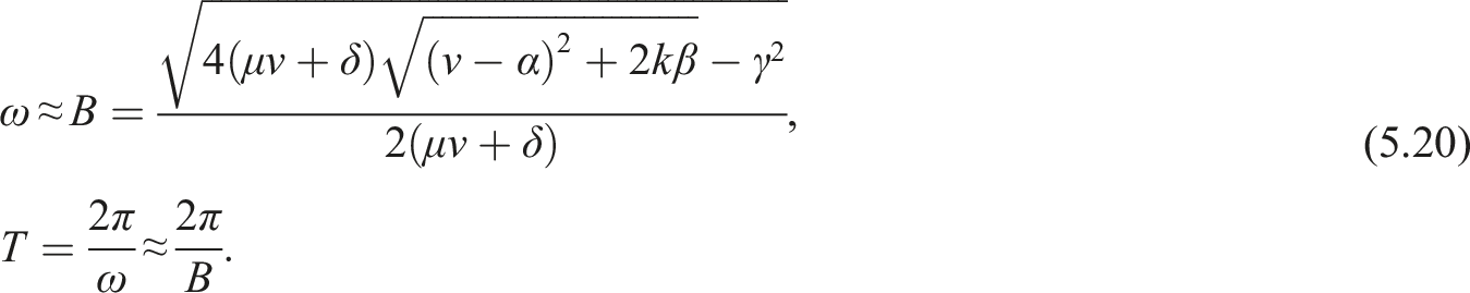
It is noticed that bigger γ² create lower vibration frequencies ω, whereas smaller γ² produce greater vibration frequencies ω. Increasing γ² results in a longer time T, whereas decreasing it results in a shorter period T. It is consistent with Figures 4–6. Using (4.3) and (4.17), we discovered that the coefficient β in the nonlinear term influences the amplitude of bounded traveling wave solutions. The amplitude of solutions decreases as β increases, and increases as β decreases.

Conclusion and prospect

Summary of this paper

In this paper, we have applied the theory of planar dynamical systems to execute comprehensive qualitative analysis for bounded traveling wave solutions of the KdV-BBM-B equation. We have also studied the existence conditions of bounded traveling wave solutions for equation (1.1) and the relationships between the behaviors of these solutions and the dissipation coefficients. And then, in some conditions, we have obtained its exact bell profile solitary wave solutions and kink profile solitary-wave solutions. An exact solution can be employed not only to check whether the methods of numerical analysis and approximation are good but also for quantitative analysis. So, it is significant to investigate exact solutions in theoretical and applied research. Beyond that we have also got the approximate damped oscillatory solutions of equation (1.1) and presented the error estimates. It is very significant to show error estimates, or else it would be considered unreliable in applied physics and mechanics. It should be pointed out that this paper has presented a method of finding the approximate damped oscillatory solutions to nonlinear evolution equations with the dissipation effect. Finding out the error estimate is the difficulty of this article, the reason is that we only know the approximate damped oscillatory solutions without its exact solutions. To overcome it, we have used some transformations and the idea of homogenization principle. Furthermore, we have established the integral equation reflecting the relation between the exact and approximate damped oscillatory solutions, and give error estimates for the approximate solutions. The errors are infinitesimal decreasing in exponential form.

Novelty of this paper

a. Previous studies on traveling wave solutions of equations mainly used the hypothesis undetermined method and the homogeneous equilibrium method. In this paper, all the bounded traveling wave solutions of the equation are studied in detail by using the theory and method of plane dynamic system;

b. In this paper, the effect of the dissipation effect on the solution state of the equation is studied. At the same time, we give the critical value or value interval to characterize the magnitude of the dissipative action, and point out the range in which the dissipative coefficient changes, the bell-like solitary wave solution, the torsional solitary wave solution or the attenuation oscillation solution will appear in the equation;

c. According to the evolution relationship of the solution orbits corresponding to the attenuated oscillation solutions in the phase diagram, we know that the generation of the attenuated oscillation solutions is essentially generated by the corresponding homologous or alien orbital rupture under the action of the dissipative term. Therefore, the structure of the attenuated oscillation solution is successfully designed on the basis of the exact bell or twisted solitaire solution of the equation without dissipative action, and the approximate solution of the attenuated oscillation solution is obtained by using the hypothesis undetermined method;

d. In order to ensure the rationality of the approximate solution of the attenuated oscillation solution, we obtained the error estimate of the approximate solution of the attenuated oscillation solution of the equation by establishing an integral equation reflecting the relationship between the approximate solution and the exact solution according to the idea of the homogenization principle. It can be seen from the error estimate that the error is an infinitesimally small amount that decreases rapidly in exponential form.

Prospects for future research work

Nonlinear wave equation is an important mathematical model to describe natural phenomena, and it is also an important hot topic in the study of soliton theory. Although this paper has made some theoretical progress in the study of nonlinear wave equations, nonlinear science is still a young subject after all, and there is still a lot of work to be studied further. Here, only a few aspects related to this paper to do the outlook, the specific work to be carried out as follows:

a. Nonlinear wave equation is a very active research field, especially the study of its corresponding dynamic behavior, but in reality, the model describing nonlinear wave equation is often affected by external forces, especially random forces; Moreover, for nonlinear wave equations, we generally analyze the bifurcation of the system solution and the corresponding solution structure through different integral processes, but the actual system may not only have parametric disturbances but also system structure disturbances. These structural disturbances may be linear (such as viscous damping term) or nonlinear. They sometimes have an essential effect on the phase diagram of the system. In view of the above problems, work on perturbation effects is planned.

b. So far, only the theory and methods of planar dynamical systems have been used to study conservative systems or dissipative systems with low order nonlinear terms. With the development of soliton theory, coupling and high-dimensional nonlinear equations have become a hot topic. Many practical models can be reduced to coupling and high-dimensional nonlinear equations. For nonlinear systems with both high-order nonlinear terms and dissipative effects, we can see that there are few papers on this research. Therefore, we need to continue to deepen and develop the research of coupled, high, and discrete nonlinear equations, which will be one of the future research directions.