
Abstract
A brief introduction to the development of the homotopy perturbation method is given, and the main milestones are elucidated with more than 90 references. This paper further improves the method by constructing a homotopy equation with one or more auxiliary parameters embedding in the linear term with a clear advantage in accelerating and controlling the approximation convergence speed. Moreover, a revision of a recent amplitude-period approximation formula is presented providing an answer to an open problem related to the optimal approximation along with a new universal formula. Duffing equation is used as an example to illustrate the solution process for the homotopy perturbation method, and only one or few iterations are needed in practical applications, making the method much attractive. From the side of amplitude-period formulation, the nonlinear pendulum, the Duffing equation and an oscillator with discontinuity are analyzed providing an asymptotic exact equivalence for bigger parameter values in the case of Duffing’s system. This mini review gives a tutorial guideline for practical applications of the homotopy perturbation method, the references are not exhaustive.
Keywords
Introduction
Nonlinear oscillations occur in many and diverse application’s fields (see for instance Cveticanin 1 and Kovacic and Brennan 2 ). The ODE’s nonlinear nature of the dynamical modeling for these oscillators makes it impossible to derive exact closed-form solutions (except for a few particular cases 3 ).
To overcome this shortcoming, several approximations were proposed in the past to count (see for instance Constantin 4 and the references therein): Homotopy perturbation, harmonic balance, a domain decomposition, variational formulation, variational iteration, pseudospectral method, Rayleigh-balance, energy-balance, max-min approach, amplitude-frequency formulation, homotopy analysis, optimal homotopy asymptotic method.
Some of these methods evidenced recent advances in the last few years. This is the case of the homotopy perturbation method proposed in 1999, 5 that has been improved by the owner through 2000 to the present.6–18
The theory has been extensively studied for decades by numerous authors, for examples Ganji and Sadighi, 19 Odibat and Momani, 20 Cveticanin, 21 Khan and Mohyud-Din, 22 to mention a few. Using Clarivate Analytics’ web of science, there are 4076 records by searching for the topic of “homotopy perturbation or HPM” until 26 December 2017.
The method has now matured into a full-fledged mathematical normative theory due to its effectiveness and simplicity. When Davood Domiri Ganji talked with ScienceWatch.com on February 2008, he said “Wherever a nonlinear equation is found, Dr He’s HPM will be the primary tool of discovery”, and “He’s perturbation method itself is mathematically beautiful and extremely accessible to non-mathematicians.”
There are many modifications of the method,23–28 according to web of science there are 338 hits by search for the topic of “modified homotopy perturbation method” and there are 113 articles on sciencedirect.com using a modified homotopy perturbation method until 26 December 2017.
The main development of the homotopy perturbation method was to adopt the parameter-expansion technology29–33 to effectively deal with the zero-order approximate and He’s polynomials to deal with the nonlinear terms.34–40
Now there is a trend to combination of the homotopy perturbation method with other methods, 18 for examples combination of the method with variational theory 41 and least squares technology. 42 The prevailing trend is to adopt the Laplace transform in the homotopy perturbation method. 43 The Laplace transform is extremely simple to deal with the linear differential equations, and the homotopy perturbation method is to change a nonlinear equation into a series of linear equations. This effective modification has been widely used in open literature with different names: Laplace transform-homotopy perturbation method,44,45 homotopy perturbation method with Laplace transform, 46 homotopy perturbation transform method, 47 homotopy perturbation Padé transform method; 36 all the above methods are actually the same method with different names. Mishra and Nagar 48 suggested this method should be called as He-Laplace method, which is extremely effective for fractional calculus.49–55
For a comprehensive review on the homotopy perturbation method, from its basic ideas, concept, skills and applications, the reader is referred to a few review articles and elementary introductions published in International Journal of Modern Physics B,8,9 Abstract and Applied Analysis 16 and International Journal of Theoretical Physics. 18
Though it becomes matured, the method has still some space for further improvement. In this paper, we will introduce an auxiliary parameter in the linear term instead of the nonlinear term to accelerate the convergence.
On the other hand, the recent method of amplitude-period approximations (see literature56–58 for instance) has witnessed great achievements. In particular, Dan and Zhi 59 present a recent review in this direction. To figure out these advances, it is worth mentioning: He’s frequency formulation (see for instance He 60 ), Max-Min approach to nonlinear oscillators (see for instance He 61 ), Taylor series (see for instance He 62 ), the simplest Amplitude-frequency formulation. 63
In this paper, two methods are reviewed: the homotopy perturbation method5–18 and the amplitude-period formula presented in García 64 with complement in Suárez Antola. 65
In both cases new research is also presented: in the homotopy case, a new way to construct a homotopy is presented, thus opening the door to multiple scales oscillators or even forced oscillators with (possible) multiple parameters; for the amplitude-period formula, the open problem in García 64 is answered using optimization for small-amplitude oscillations, but also a necessary condition to provide explicit universal amplitude-period approximation formulas with exact asymptotic behavior.
Homotopy perturbation method
Consider the following general differential equation


The homotopy analysis method66,67 introduces an auxiliary parameter in the form


For any non-zero h, equation (5) is equivalent to the original one. It requires skill to optimally choose the value of h because h can be any real number except zero. Though it can be freely chosen for an infinite series solution, e.g. h = 0.0001 or h = –0.0001 or h = 10,000, the choice of h will greatly affect the asymptotic property of a finite series solution. There are many publications on how to identify the value of h, and the prevailing method is the h-curve method.66,67
For nonlinear oscillator, equation (2) does not work. As an example, we consider the Duffing equation

If a homotopy equation is constructed in the form


For absence of the linear term in an equation, for example He
9

We can only obtain a series of solution instead of a periodic solution if the following homotopy equation is constructed

To solve the problem, the parameter-expansion method29–33 can be used. We re-write equation (9) in the form

The coefficient, zero, of u in the missing linear term can be expanded in a series of p29–33


When p = 1, equation (11) returns to be the original one. So, the solution process is to deform a linear oscillator with an unknown frequency when p = 0 to the original one when p = 1. This process converges very fast, and only one iteration is always enough for most problems, though iteration can continue without any difficulty to obtain higher order approximate solutions.
For a nonlinear oscillator with a negative linear term, for example


The above remarks reflect the development of the homotopy perturbation method. The most important step in the homotopy perturbation method is to construct a suitable homotopy equation with a possible one free parameter. For equation (1) the general construction of the homotopy perturbation method is11–13


An auxiliary parameter in the homotopy perturbation method
An auxiliary parameter was introduced in the variational iteration method68–71 and the homotopy perturbation method 72 to accelerate convergence. Some special technologies have been developed to optimally determine the auxiliary parameter by the least square method or other collocation methods, and modifications are called as the optimal variational iteration method73–77 and optimal homotopy perturbation method.25,78–82 This paper suggests an alternative construction of homotopy equation with an auxiliary parameter. This is an extension of the homotopy perturbation method with an auxiliary term 15 and homotopy perturbation method with two expanding parameters. 17
We re-write equation (1) in the form


For the well-known Duffing equation, the homotopy equation is constructed in the form

We assume that the solution can be expanded into a series of p in the form

Submitting equation (22) into equation (21), and manipulating as the classic perturbation method does, we have


Solving equation (23), we have

Substituting equation (25) into equation (24) results in

By a simple operation, we have

No secular term in
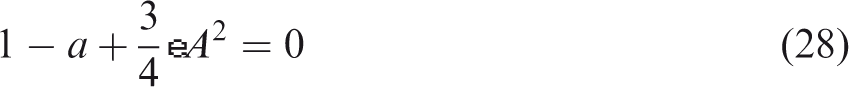
Solving a from equation (28) yields the result
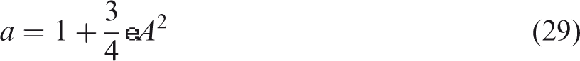
We, therefore, obtain the following approximate solution
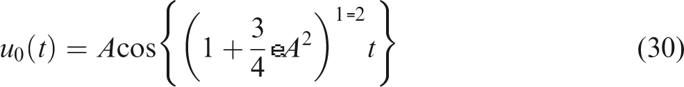
When
Amplitude-period formulation: García’s formula and improvements
As discussed in previous sections, the homotopy equation given in Equation (2) is not working for nonlinear oscillators. As described, several methods including the novel way to construct the homotopy using an auxiliary parameter in this paper overcome this shortcoming.
On the other hand and recently developed, simple amplitude-period formulas can be also considered to study nonlinear oscillators (see for instance literature58,63–65,83–85)
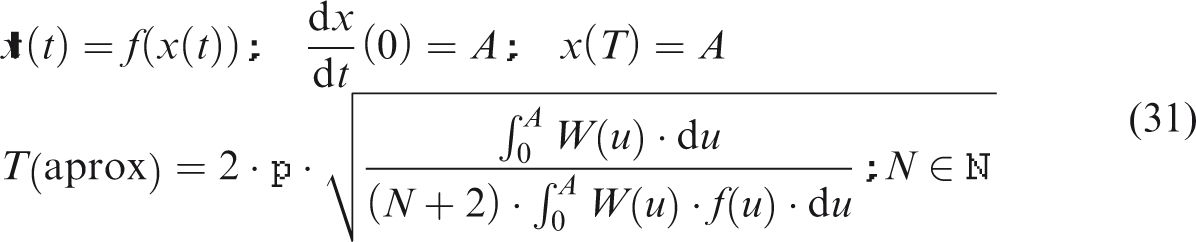
When W(x) takes the form
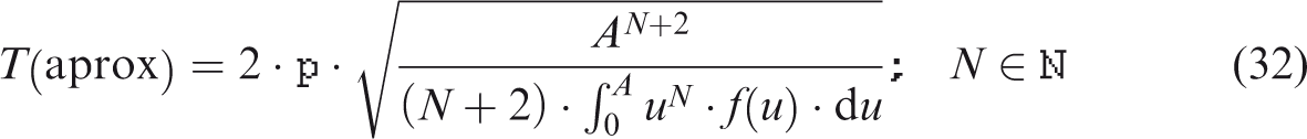
In García
64
an open problem was posed to prove or disprove whether or not equation (32) is an optimal approximation to the true amplitude-period relationship with N = 3. To provide an answer to this problem when
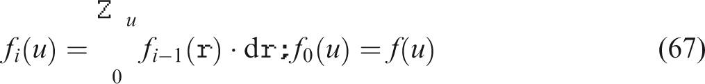
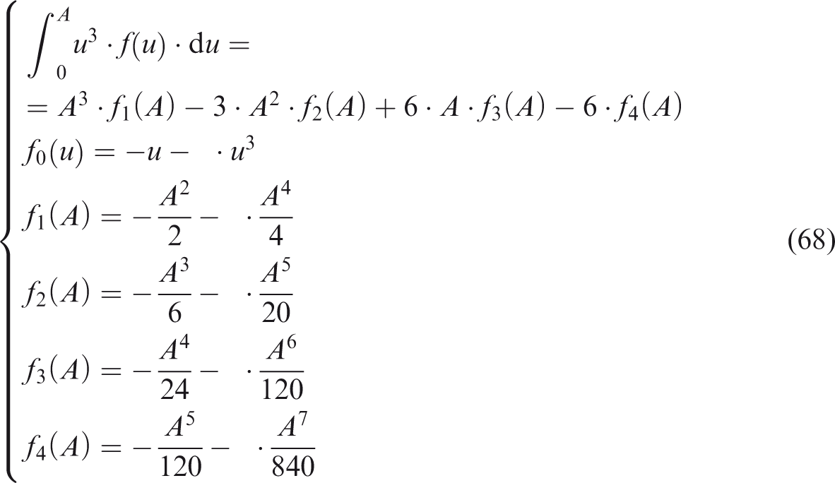
Taking the integration

Naming
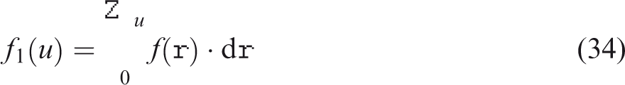
Equation (33) becomes
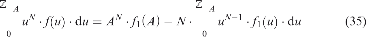
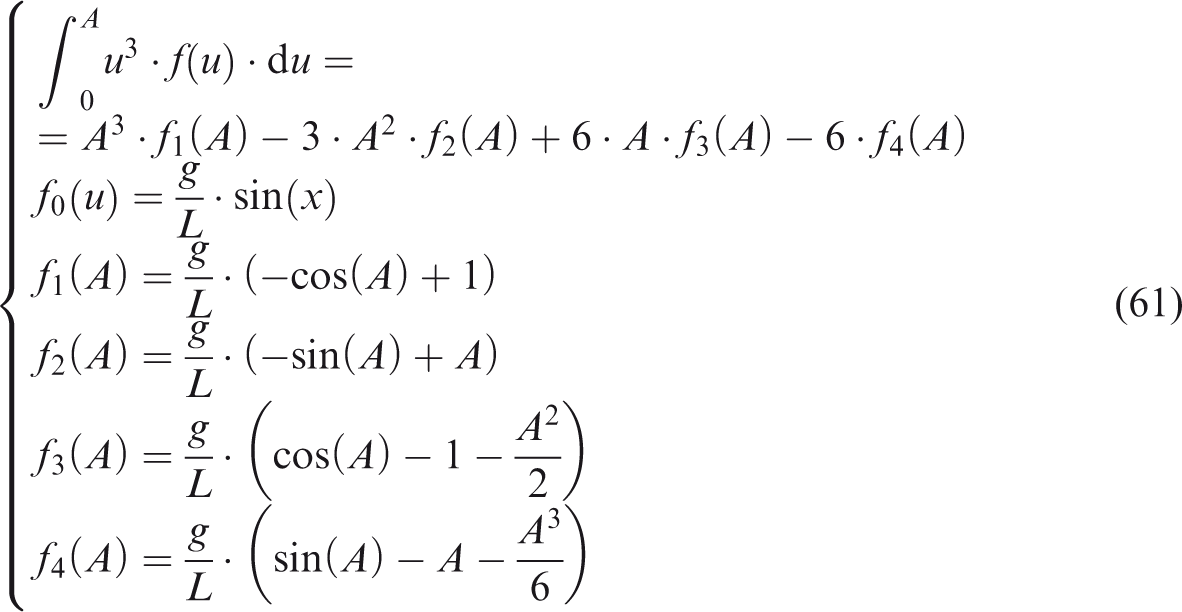
Integrating again by parts
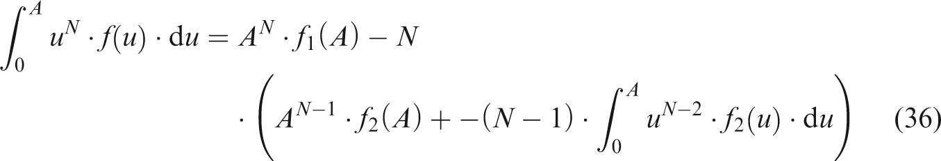
With
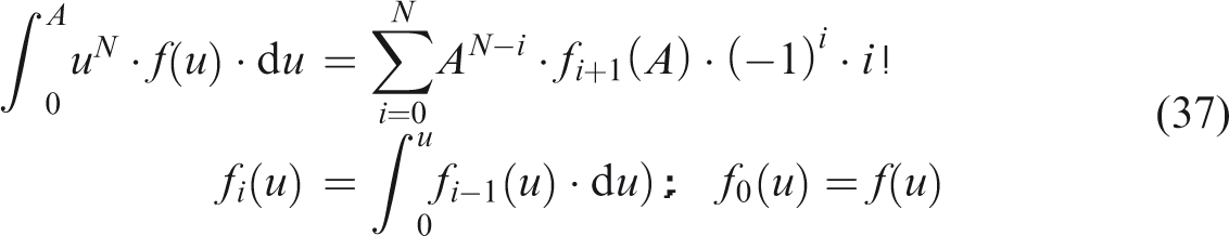
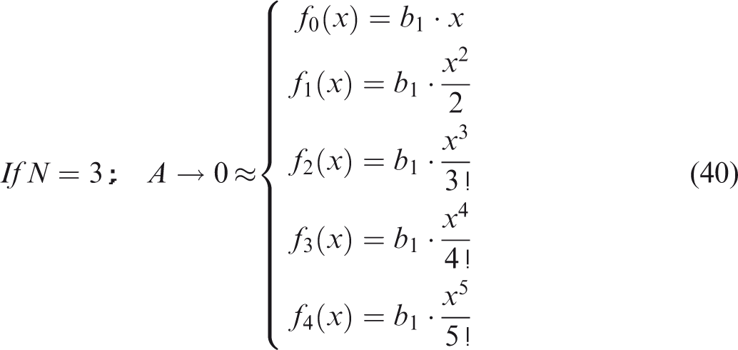
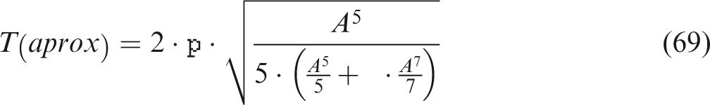
Utilizing equation (37) and assuming that
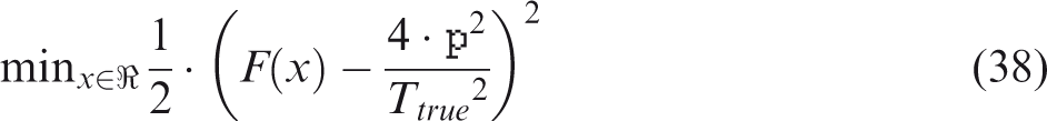

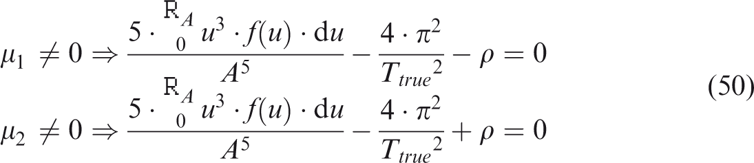
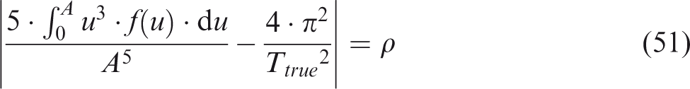
It is important to remark that the optimal problem requests for a possible local extremum satisfying equation (39) in the interval:
Then

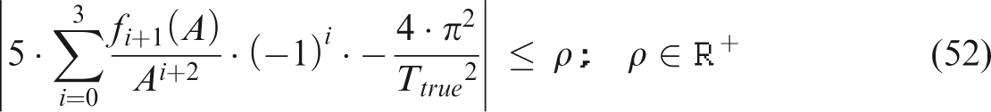
Simplifying

With roots

Clearly, the integer approximation of the third roots gives the desired result. This completes the proof.
Notice that the theorem is valid even for infinite series representation:
Then

The Karush-Kuhn-Tucker conditions read
Since (see for instance García
64
)
It is clear that
In other words
This completes the proof, taking the minimum/maximum roots of this equation.
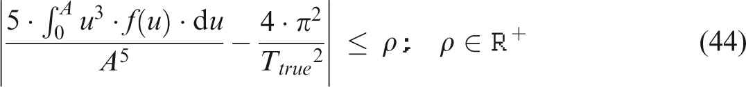
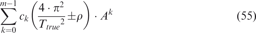
The important remark is about the universality nature of equation (44) providing amplitude-period approximations with a given error bound. Moreover, when the nonlinear oscillator is polynomial:
Then


Proof:
According to Theorem 2 and the proof in Theorem 1 it is enough to consider bounds for the maximum and minimum positive roots of a polynomial (see for instance Cohen
86
). Finally performing the change:
Results and discussion
Homotopy method with auxiliary parameters
The homotopy perturbation method always stops before second iteration; however, iterations can be continued without any difficulties. If higher order approximates solutions are needed, equation (19) can be extended to more than one auxiliary parameter, for example if a second-order approximate solution is searched for, the homotopy equation can be written in the form

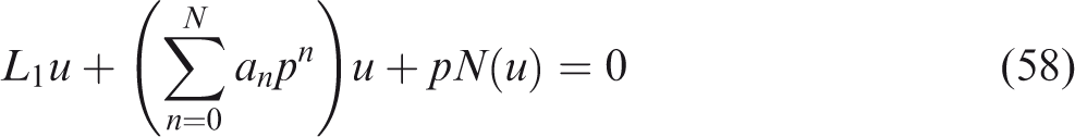
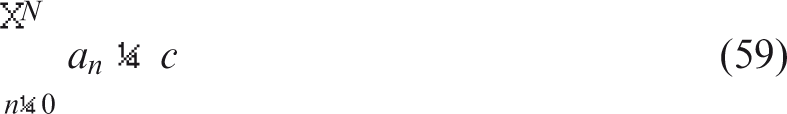
For N-th order approximate solution, we have

The present technology can be easily extended to the multiple scales homotopy perturbation method 87 to deal with forced oscillators.
Amplitude-period formulation
Nonlinear pendulum
The nonlinear pendulum is always a source for testing approximations (see for instance Beléndez et al.
3
)
Applying equation (37) and Theorem 1

Finally
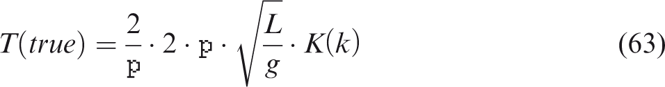
Whereas the true amplitude-period relationship is (see Beléndez et al.
3
)
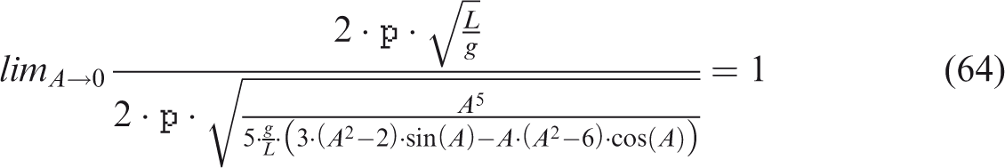

This means, zero error.
Duffing oscillator
To show the improved formula’s applicability, the classical Duffing oscillator is analyzed (see for instance Kovacic and Brennan
2
)

Applying Theorem 2
Hence
Finally
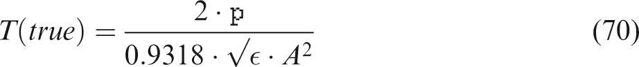
Whereas the true amplitude-period relationship for

Moreover, equation (55) reads
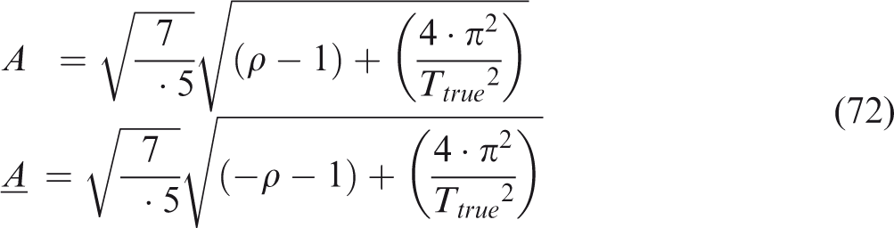
Giving the following bounds
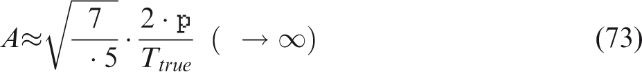
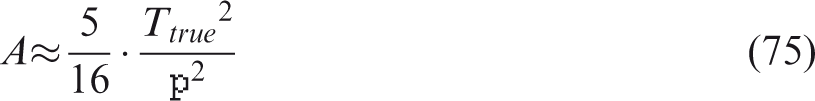
If

The clear and important implication is that Theorem 2 provides an asymptotic equivalence between Garcia’s formula and the true amplitude-period relationship when the parameter
An oscillator with discontinuity
To continue with the asymptotic equivalence, let us consider the following oscillator

Comparing with the true amplitude-period relationship (see García
64
)
The asymptotic approximation is very precise (about 98.69%).
There are many alternative approaches to nonlinear oscillators, an answer was given to the open problem that appeared in García 64 about an amplitude-period formula for small amplitude period oscillations (Theorem 1). The technique can be extended to improve the theorem for non-small oscillations taking into account the universal bounds presented in Theorem 2 and Corollary 1.
It should also be pointed out that the nonlinear oscillation community finds a road to Rome by simple frequency-amplitude formulations discussed in Nonlinear Science Letters A64,65 and literature.63,83–86
Conclusions
In this paper, we suggest a novel way to construct a homotopy equation with one or more auxiliary parameters. The new formulation's salient property relies on the possibility to control or even accelerate the convergence of the approximations.
This idea can be extended to other nonlinear problems, and the present paper can be used as a paradigm for other applications.
Finally, the Garcia’s formula along with the universal bounds given in Theorem 1 makes such a formulation very promising from the computer implementation point of view. The methods discussed in this paper can be easily extended to fractional differential equations.88–92
Footnotes
Declaration of conflicting interests
The author(s) declared no potential conflicts of interest with respect to the research, authorship, and/or publication of this article.
Funding
The author(s) disclosed receipt of the following financial support for the research, authorship, and/or publication of this article: The work is supported by Priority Academic Program Development of Jiangsu Higher Education Institutions (PAPD), National Natural Science Foundation of China under grant No.11372205 and Universidad Tecnológica Nacional.