An adaptive algorithm,based on modified tanh non-linearity and fractional processing,for impulsive active noise control systems

Abstract

This paper presents an adaptive algorithm for active control of noise sources that are of impulsive nature. The impulsive type sources can be better modeled as a stable distribution than the Gaussian. However, for stable distributions, the variance (second order moment) is infinite. The standard adaptive filtering algorithms, which are based on minimizing variance and assuming Gaussian distribution, converge slowly or become even unstable for stable (impulsive) processes. In order to improve the performance of the standard filtered-x least mean square (FxLMS)-based impulsive active noise control (IANC) systems, we propose two enhancements in this paper. First, we propose employing modified tanh function-based nonlinear process in the reference and error paths of the standard FxLMS algorithm. The main idea is to automatically give an appropriate weight to the various samples in the process, i.e. appropriately threshold the very large values so that system remains stable, and give more weight to samples below threshold limit so that the convergence speed can be improved. A second proposal is to incorporate the fractional-gradient computation in the update vector of IANC adaptive filter. Computer simulations have been carried out using experimental data for the acoustic paths. The simulation results demonstrate that the proposed algorithm is very effective for IANC systems.

Introduction

According to a technical report by World Health Organization (WHO), ¹ noise pollution is a serious environmental challenge and severely affects human health. The traditional means of noise reduction are termed as passive noise absorbers, where noise mitigation is achieved by employing absorbing materials to “absorb” the unwanted noise. Essentially, the unwanted acoustic noise is damped out by converting it to the other form of energy, e.g. heat. The passive noise absorption works well for a high-frequency noise source; however, it is costly and bulky for controlling the noise sources that are in a low-frequency range.^2,3 The acoustic dampers find application in modern combustion systems, where coupling between the unsteady heat release and the acoustic waves may cause thermoacoustic instability.^4–6 The acoustic dampers are employed to reduce the engine noise, and hence stabilize the combustion system. ⁷ In contrast to the passive means of damping acoustic noise, the active techniques rely on generating an appropriate “anti-noise” signal, hence the name “active.” The basic idea is quite simple and well known in Physics: a destructive interference happening between two waves of equal magnitude and opposite phases results in cancellation of both. The concept that the destructive interference of acoustic waves can be employed to perform acoustic noise cancellation was first proposed in a US patent by Lueg. ⁸ However, the early analog techniques did not result in successful applications for efficient noise cancellation in actual practice. The advancements in digital signal processing (DSP) algorithms as well as hardware implementation, over the past few decades, have resulted in successful noise cancellation systems for many practical applications, viz., air conditioning ducts, cars, aircrafts, headphones, and so on.^9–14

The most successful scenario for active control of acoustic noise is a single-channel situation, which comprises one primary (reference) microphone, one secondary (cancelling) loudspeaker, and one error microphone. The reference microphone picks-up the reference noise in advance. The primary noise propagates via the so-called primary acoustic path to the location of error microphone where the noise reduction is in fact desired. The secondary (cancelling) signal generated by the control filter (which is in fact an adaptive filer, as explained later) propagates via the so-called secondary (electro-acoustic) path. The objective of the control filter is to generate an appropriate (anti-phase) signal which would result in the cancelling of primary noise, and hence a reduction of the sound pressure level at the location of the error microphone. Finally, the error microphone senses the result of destructive interference between the acoustic waves.

Due to the time-varying nature of acoustic environment, for example, variations in humidity, airflow, temperature, etc., the adaptive filtering plays a pivotal role in the practical active control systems. The standard adaptive filtering algorithms, however, do not perform well due to the presence of the secondary path between the generation of the cancellation signal and pick-up of the residual error signal. The celebrated least mean square (LMS) algorithm, ¹⁵ which is based on minimization of variance of the error signal, has been modified to compensate for the effect of secondary path transfer function. This has resulted in a filtered-reference version, where the reference signal is being filtered via model of the secondary path. The filtered-x reference LMS (most commonly known as FxLMS) algorithm requires low computational efforts and is simple to implement. However, the standard FxLMS algorithm does not perform well for impulse-type noise sources as considered in this paper.

The impulsive noise is characterized by occurrence of low probability large value samples. Such noise sources occur in many practical environments, for example, heavy machinery in industrial setup, traffic noise, gun shot and explosion, noise in MRI room, and so on. ¹⁶ In the recent literature on impulsive active noise control (IANC), it is a usual practice to model such impulse-type noise using symmetric alpha stable (SαS) distribution. A random process is termed as SαS, if characteristic function can be expressed as ¹⁷

$$\varphi (t)=e^{(\mathit{jat}-\gamma |t{|}^{\alpha })}$$

(1) where $-\infty <a<\infty$ is called the location parameter, γ is the scale parameter, and $0<\alpha \le 2$ is the characteristic exponent. By taking inverse Fourier transform of the characteristic function $\varphi (t)$ , the corresponding probability density function (PDF) can be computed; however, a closed form expression does not exist is general, except for α = 1 and α = 2 for which the corresponding PDF is Cauchy and Gaussian, respectively. ¹⁷ If a = 0 and γ = 1, then the corresponding SαS distribution is called standard. In this paper, we consider the noise source being modeled as a standard SαS distribution, where the characteristic exponent α controls the impulsive nature: low value of α indicating highly impulsive sources and $\alpha \to 2$ indicating source with a less impulsive nature and close to Gaussian distribution.

The impulsive noise is very dangerous as it can cause temporary or even a permanent hearing loss. Therefore, it is very important to develop efficient IANC algorithms and systems to mitigate impulsive noise. ¹⁸ The same applies to building and/or heavy industrial equipment with possibly vibrating structures/panels, ¹⁹ where high impact shocks can cause severe damage. The results presented in this paper equally apply to impulsive active vibration control (IAVC); however, we stick to IANC for acoustic noise sources and the interested reader may extend the methods and results to develop IAVC systems. For some other interesting applications of LMS-based adaptive filtering, the reader is referred to Zhao and Chow ²⁰ and Li et al. ²¹

For stable processes, the variance is infinite, i.e. the second order moments do not exist, and hence the FxLMS algorithm (which is a variant of LMS algorithm) does not give a stable performance. Broadly speaking, there are two approaches to develop stable adaptive algorithms for IANC: (1) derive the adaptive algorithm by minimizing lower fractional order moment $p<\alpha$ (which does exist for stable distributions) resulting in Fx-least mean p-power (FxLMP) algorithm ²² and (2) improve robustness of the standard FxLMS algorithm by properly thresholding the reference and/error signals.^23,24 The FxLMP algorithm and its variants ²⁵ require estimating p in relation with α, which might not be possible in some practical scenarios. Due to this reason, we consider developing a variant of the FxLMS algorithm for IANC.

In the proposed algorithm discussed in this paper, the first idea is to apply a (modified) tanh function-based non-linearity to process the reference and error signals in the update equation of the FxLMS algorithm. Furthermore, we suggest incorporating fractional-processing-based gradient computation in the update equation of the proposed algorithm. Introducing the underlying concepts of fractional calculus^26–28 in the field of signal processing belongs to Ortigurea.^29,30 Recently, the fractional adaptive strategies have been developed and employed for secondary path modeling filter in active noise control systems, ³¹ for Hammerstein nonlinear ARMAX systems ³² and identification of CARMA model. ³³ The fractional-calculus-based modified versions of LMS algorithms have also been independently proposed in literature.^34,35 The interesting results in Aslam and Raja ³¹ have motivated us to exploration and exploitation of fractional signal processing for designing effective adaptive algorithm for IANC systems. In order to demonstrate the effectiveness of the proposed algorithm, the computer simulations have been carried out with the experimental data for the acoustic paths.

The rest of the paper is organized as follows. The next section gives a brief overview of ‘IANC Using FxLMS and previous algorithms’. The details of the proposed algorithm are given in ‘Development of proposed IANC algorithm’. ‘Simulation results’ section describes the numerical results and discusses performance comparison for various IANC algorithms, followed by conclusions presented in ‘Concluding remarks’ section.

IANC using FxLMS and previous algorithms

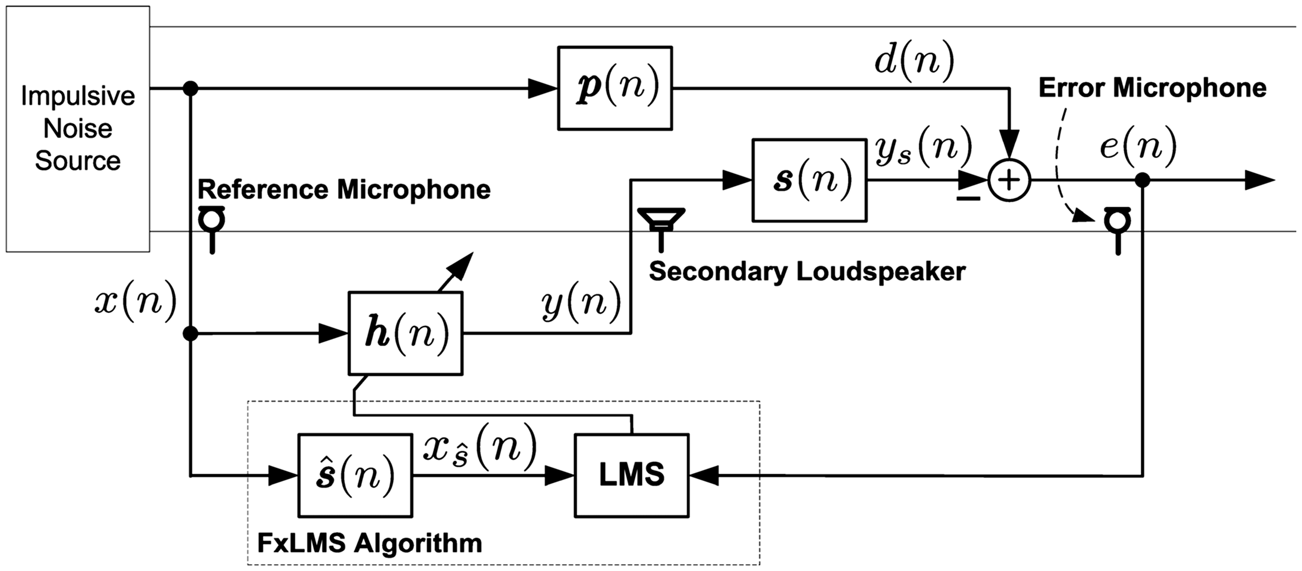
Figure 1 presents a schematic diagram for a single-channel IANC system in a feedforward configuration for duct applications, for example. Here, $p(n)$ denotes impulse response coefficient vector of the primary acoustic path where discrete time index n is used to indicate that the acoustic path may in fact be having time-varying characteristics. Similarly, the secondary path is represented by the impulse response coefficient vector $s(n)$ . The reference signal x(n) (via primary path $p(n)$ ) appears as a primary disturbance signal d(n) at location of the error microphone. The output signal y(n) from the IANC adaptive filter $h(n)$ is filtered via $s(n)$ to provide the noise cancellation around the error microphone and to produce the residual error signal e(n). These operations can be expressed as

$$d(n)=p^T(n)x(n)$$

(2)

$$y_s(n)=s^T(n)y(n)$$

(3)

$$e(n)=d(n)-y_s(n)$$

(4) where $p(n)=[p_0(n),p_1(n),\dots ,p_{L-1}(n){]}^T$ is the coefficient vector for the primary path being modeled as a finite impulse response (FIR) filter of length L, $s(n)=[s_0(n),s_1(n),\dots ,s_{M-1}(n){]}^T$ is the coefficient vector for the secondary path being modeled as an FIR filter of length M

$$x(n)=[x(n),x(n-1),\dots ,x(n-i+1){]}^T$$

(5) is the (i = L) sample input signal vector and $y(n)=[y(n),y(n-1),\dots ,y(n-M+1)]$ is the signal vector comprising M recent samples of the output signal y(n) being computed as

$$y(n)=h^T(n)x(n)$$

(6) where $h(n)=[h_0(n),h_1(n),\dots ,h_{L_h-1}(n){]}^T$ is the coefficient vector for the adaptive IANC filter being considered as an FIR filter of length L_h, and $x(n)$ is the input signal vector as given in equation (5) with i = L_h. It is important to note that the computations in equations (2) to (4) are being carried out in the acoustic domain, and we have access only to the residual error signal e(n) being picked up by the error microphone. By minimizing mean square value of the error signal e(n), the corresponding update equation for the FxLMS algorithm is obtained as ⁹

$$h(n+1)=h(n)+\mu e(n)x_{\hat{s}}(n)$$

(7) where μ is the step-size parameter, and

$$x_{\hat{s}}(n)=[x_{\hat{s}}(n),x_{\hat{s}}(n-1),\dots ,x_{\hat{s}}(n-L_h+1){]}^T$$

(8) is the vector for the filtered-reference signal $x_s(n)$ being computed as

$$x_{\hat{s}}(n)={\hat{s}}^T(n)x(n)$$

(9) where $\hat{s}(n)=[{\hat{s}}_0(n),{\hat{s}}_1(n),\dots ,{\hat{s}}_{M-1}(n){]}^T$ denotes coefficients of the secondary path modeling filter $\hat{s}(n)$ which is assumed as an FIR filter of the same length M as that of the secondary path $s(n)$ , and $x(n)$ is the corresponding (i = M)-length input signal vector as given in equation (5). The FxLMS algorithm requires computing two filtering operations: the output signal y(n) in equation (6) and the filtered-reference signal $x_{\hat{s}}(n)$ in equation (9). The reference signal used in these computations is given in equation (5), where we observe that all samples have been treated “equally” regardless of their magnitude at difference times. In the case of impulsive noise sources, some of the samples may exhibit excessively large magnitude and may severely perturb the operation of IANC system. In the worst case scenario, the IANC system may become unstable. ²³ The stability can be improved by choosing a very small value for the step-size parameter μ; however, this in turn would degrade the convergence speed.

Figure 1.

Schematic diagram of single-channel impulsive active noise control (IANC) system employing standard FxLMS algorithm.

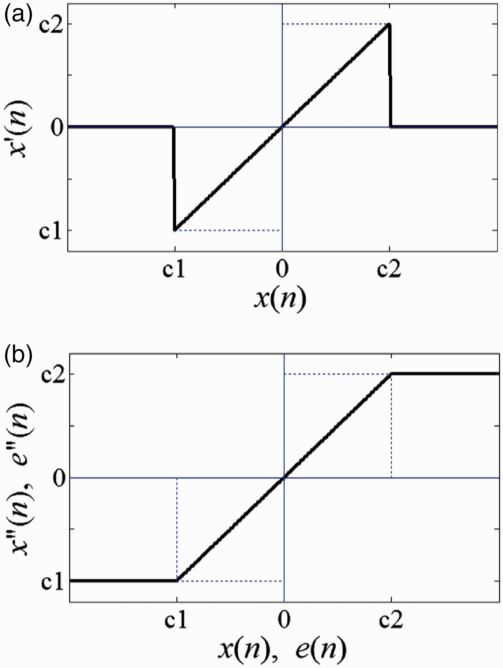
One of the earlier attempts to improve stability and convergence performance of the standard FxLMS algorithm for IANC systems is due to Sun et al. ²³ proposing employing truncation non-linearity for the input signal as

$$\begin{array}{c}\multicolumn{1}{c}{x\text{'}(n)=\{\begin{array}{cc}x(n);& \hfill \text{ if }x(n)\in [c_1,c_2]\hfill \\ 0;& \hfill \text{otherwise}\hfill \end{array}}\end{array}$$

(10) where $[c_1,c_2]$ are the thresholding parameters (see Figure 2(a)). Thus, in Sun’s algorithm, the samples of the filtered-reference signal $x_{\hat{s}}(n)$ are computed as

$$x_{\hat{s}}(n)={\hat{s}}^T(n)x\text{'}(n)$$

(11) where $x\text{'}(n)=[x\text{'}(n),x\text{'}(n-1),\dots ,x\text{'}(n-M+1){]}^T$ is the modified reference signal vector, whose sample are computed by the truncation non-linearity as given in equation (10). Finally, weights of the IANC adaptive filter $h(n)$ are updated using FxLMS algorithm of equation (7). Sun’s algorithm improves the stability of the FxLMS algorithm-based IANC system; however, it takes care of peaky samples only while computing the filtered-reference signal $x_{\hat{s}}(n)$ in equation (9). The peaky samples may propagate to the residual error signal e(n), especially at the startup of IANC system, or when there is a change in the acoustic environment. Employing a similar truncation non-linearity as given in equation (10) to the error signal e(n) will effectively freeze the adaptation when a large value beyond $[c_1,c_2]$ appears in the error signal. Furthermore, ignoring the samples might result in a loss of some desired information.

Figure 2.

(a) Truncation non-linear transformation for the reference signal x(n) in Sun’s modified-FxLMS algorithm. ²³ (b) Saturation non-linear transformation for the reference signal x(n) and the error signal e(n) in previous algorithm. ²⁴

In order to overcome the above-mentioned issues, the previous algorithm ²⁴ employs saturation non-linearity, as shown in Figure 2(b), in both the filtered-reference and error signals. The samples of the filtered-reference signal ${\hat{x}}_s(n)$ are computed as

$$x_{\hat{s}}(n)={\hat{s}}^T(n)x″(n)$$

(12) where

$$x″(n)=[x″(n),x″(n-1),\dots ,x″(n-M+1){]}^T$$

(13) is the modified reference signal vector, whose samples are computed by filtering a saturation non-linearity as $x″(n)=\lfloor x(n){\rfloor }_{c_1}^{c_2}$ , which replaces the samples below c₁ with lower limit c₁ and samples larger than c₂ are replaced with the upper limit c₂. Similarly, the residual error signal is modified as $e″(n)=\lfloor e(n){\rfloor }_{c_1}^{c_2}$ , and finally the IANC adaptive filter is updated as ²⁴

$$w(n+1)=w(n)+\mu e″(n)x_{\hat{s}}(n)$$

(14) where $x_{\hat{s}}(n)$ is computed as in equation (12).

Development of proposed IANC algorithm

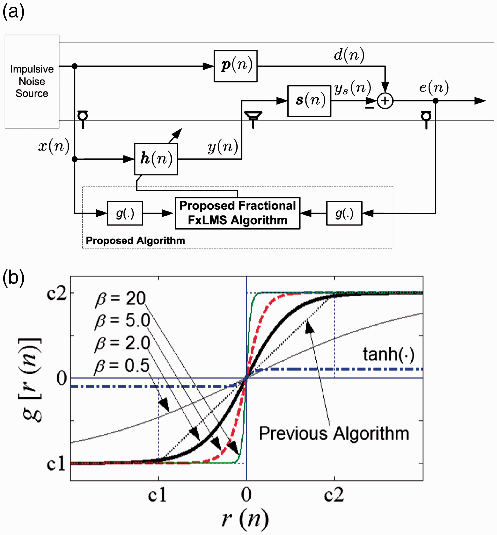
Figure 3(a) represents the configuration of the proposed IANC algorithm, which comprises two modifications in the previous algorithm. ²⁴

Figure 3.

(a) Configuration of proposed algorithm for IANC systems. (b) The tanh function-based modified saturation non-linear transformation for the reference signal x(n) and the error signal e(n) in the proposed algorithm.

Modified Tanh nonlinearity for thresholding

In this paper, we propose employing following (modified) tanh function

$$g(r(n))=k_r\mathit{tanh}(\beta \frac{r(n)}{k_r})$$

(15) where r(n) is the signal of interest, k_r is the scaling parameter which sets the steady-state value as well as controls the slope, and $\beta >0$ is a constant that provides tuning of the slope. In equation (15), the scaling parameter k_r is selected as

$$\begin{array}{c}\multicolumn{1}{c}{k_r=\{\begin{array}{cc}{c}_1;& \hfill r(n)\ge 0\hfill \\ c_2;& \hfill r(n)<0\hfill \end{array}}\end{array}$$

(16)

Figure 3(b) shows non-linear transformations $g(·)$ for the reference and error signals in the proposed method, where curves for the saturation non-linearity of previous algorithm and the standard tanh function are also included for comparison. It is evident that β = 2 results in a transformation which ensures that the large samples beyond $[c_1,c_2]$ are thresholded appropriately, as well as the rest of the samples are boosted as compared with the previous algorithm. The parameter β is, therefore, empirically selected as β = 2. A one-step further modification is suggested to employing fractional processing-based gradient computation as explained below.

Fractional FxLMS algorithm

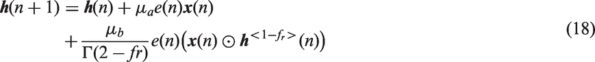
The fractional LMS (FrLMS) algorithm is a variant of the LMS algorithm, where the concept of fractional calculus has been incorporated with the gradient computation. Essentially, the update equation is modified as

$$h(n+1)=h(n)-{\mu }_a\frac{\partial J(n)}{\partial h(n)}-{\mu }_b\frac{{\partial }^{f_r}J(n)}{\partial h(n{)}^{f_r}}$$

(17) where μ_a is the step-size parameter corresponding to the ordinary gradient-based term as found in the standard LMS algorithm, and μ_b is the step-size parameter for the fractional-order gradient-based term. Considering mean square error as a cost function and performing some easy algebraic steps, the FrLMS algorithm is derived as ^{31 a}

$$\begin{array}{c}\multicolumn{1}{c}{h(n+1)=h(n)+{\mu }_{a}e(n)x(n)}\\ \multicolumn{1}{c}{+\frac{{\mu }_b}{\Gamma (2-\mathit{fr})}e(n)(x(n)\odot h^{<1-f_r>}(n))}\end{array}$$

(18) where ⊙ denotes element-wise multiplications of two vectors, $(·{)}^{<1-f_r>}$ denotes element-wise power computation, and $\Gamma (·)$ denotes the Gamma function. Thus, the FrLMS algorithm would require three parameters: (1) the step-size parameter μ_a for the ordinary gradient-based term, (2) the step-size parameter μ_b for the fractional gradient-based term, and (3) the fractional derivative-order f_r. It may be easier to tune a single parameter μ in the LMS algorithm as compared with tuning three parameters in the FrLMS algorithm. However, on the other hand, the FrLMS algorithm offers more degree of freedom, and with an appropriate setting of these parameters, it considerably improves the performance. This is indeed demonstrated by the recent research results,^31–33 that the FrLMS algorithm gives plausible performance as compared with the standard counterpart, i.e. the LMS algorithm. Motivated by these research results, we implement this idea for adapting the IANC filter $h(n)$ . Thus, a fractional modified-Tanh FxLMS algorithm, hereafter referred as the proposed algorithm, is developed with the update equation being given as

$$h(n+1)=h(n)+\mu e″(n)\{x_{\hat{s}}(n)+\delta (x_{\hat{s}}(n)\odot h^{<1-f_r>}(n))\}$$

(19) where $\delta >0$ is a positive constant for the step-size with the fractional gradient-based term. As compared with the original formulation of FrLMS algorithm given in equation (18) (see equation (22) in Widrow and Stearns ¹⁵ ), we may note the following differences:

1. Due to the presence of the secondary path $s(n)$ following the IANC adaptive filter $h(n)$ , the reference signal x(n) cannot be directly used in the update equation. Hence, filtered-reference signal $x_{\hat{s}}(n)$ is used, as in other algorithms discussed in IANC using FxLMS and previous algorithms section. It is worth to mention that $x_{\hat{s}}(n)$ is computed as in equation (12), where the samples of the modified reference signal vector $x″(n)$ in equation (13) are computed as $x″(n)=g(x(n))$ , i.e. by applying the proposed thresholding non-linearity $g(·)$ given in equation (15).

2. The error signal $e″(n)$ is computed by employing the proposed thresholding non-linearity as $e″(n)=g(e(n))$ .

3. The original formulation of FrLMS algorithm requires adjusting two separate step-size parameters μ_a and μ_b, for the terms corresponding to the ordinary and fractional gradients, respectively. We suggest to use the same step-size μ, and adjustments in the step-size for fractional gradient-based term are made by selecting $\delta >0$ . Furthermore, we assume that the normalization term $\Gamma (2-f_r)$ is being absorbed in the step-size calculation.

Summary of the proposed algorithm

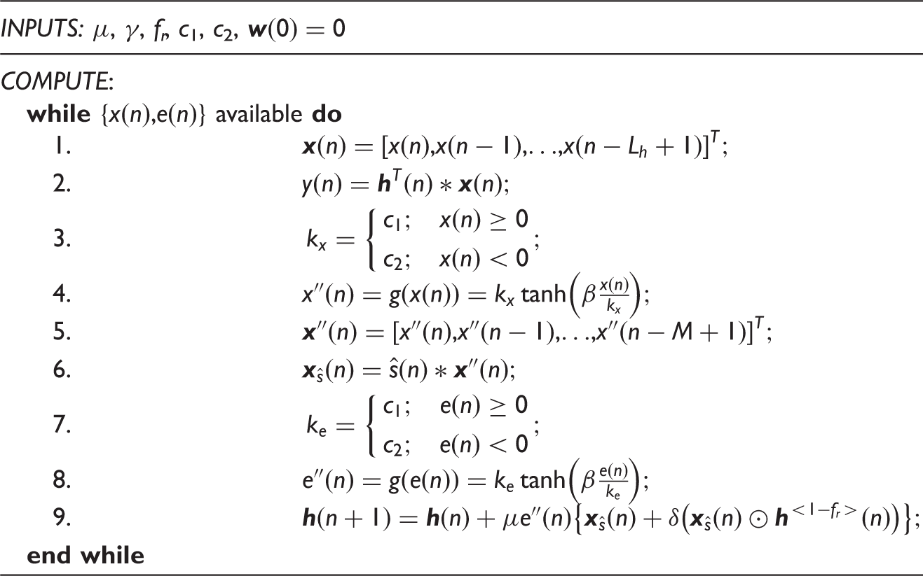
The summary of the proposed algorithm for IANC systems is given in Table 1. As discussed earlier, the proposed algorithm described in this paper comprises two strategies for improving the convergence and stability of IANC systems. The first idea is to use (an appropriate) non-linearity in the reference as well as error signal paths (see computations # 4 and 8 in Table 1).

Table 1.

Summary of the proposed algorithm for IANC systems.

INPUTS: μ, γ, fr, c1, c2, $w(0)=0$
COMPUTE:
while $\{x(n),e(n)\}$ available do
1.	$x(n)=[x(n),x(n-1),\dots ,x(n-L_h+1){]}^T;$
2.	$y(n)=h^T(n)*x(n);$
3.	$\begin{array}{c}\multicolumn{1}{c}{k_x=\{\begin{array}{cc}{c}_1;& \hfill x(n)\ge 0\hfill \\ c_2;& \hfill x(n)<0\hfill \end{array};}\end{array}$
4.	$x″(n)=g(x(n))=k_x\mathit{tanh}(\beta \frac{x(n)}{k_x});$
5.	$x″(n)=[x″(n),x″(n-1),\dots ,x″(n-M+1){]}^T;$
6.	$x_{\hat{s}}(n)=\hat{s}(n)*x″(n);$
7.	$\begin{array}{c}\multicolumn{1}{c}{k_e=\{\begin{array}{cc}{c}_1;& \hfill e(n)\ge 0\hfill \\ c_2;& \hfill e(n)<0\hfill \end{array};}\end{array}$
8.	$e″(n)=g(e(n))=k_e\mathit{tanh}(\beta \frac{e(n)}{k_e});$
9.	$h(n+1)=h(n)+\mu e″(n)\{x_{\hat{s}}(n)+\delta (x_{\hat{s}}(n)\odot h^{<1-f_r>}(n))\};$
end while

Note: Here k_x and k_e denote the constant k_r in equation (16) computed for x(n) and e(n), respectively.

The second idea is to employ the fractional gradient-based term where fractional power of the coefficient vector $h(n)$ of IANC filter is computed (element-wise) (see computation # 9 in Table 1). Essentially, the proposed algorithm may be considered as a filtered-x extension of FrLMS algorithm, which furthermore incorporates an efficient thresholding of the reference signal x(n) and error signal e(n) to make the proposed algorithm well suited for IANC systems. The proposed algorithm ensures avoiding drastic fluctuations in the coefficients of IANC filter $h(n)$ while working in an impulsive environment. This remark is supported by the results of extensive computer simulations as presented in the next section.

Simulation results

In the results presented below, the experimental data provided by Kuo and Morgan ⁹ are used to model the acoustic paths. The data in Kuo and Morgan ⁹ are a pole-zero model with numerator and denominator polynomials each of order 25. In this paper, the corresponding FIR representation is obtained by truncating the impulse responses of given model. Essentially, using the given data, the primary acoustic path $p(n)$ and the secondary acoustic path $s(n)$ are modeled as FIR filters of lengths L = 256 and M = 128, respectively. The offline measurements are an integral part of any practical active noise control systems; ⁹ therefore, we assume that the secondary path is identified offline and is available as $\hat{s}(n)=s(n)$ . The IANC adaptive filter $h(n)$ is an FIR filter of length L_h = 192. The reference signal x(n) is generated as a standard SαS process with various values of characteristic exponent α. The values for the step-size parameters are found experimentally on trial-n-error basis for fast and stable convergence, and the results are ensemble averaged for 30 runs.

It is worth mentioning that estimating the distribution parameters for the given stable process is beyond the scope of this paper. The interested reader is referred to Simmross-Wattenberg et al. ³⁶ and references therein. For IANC systems, the estimation of distribution parameters during online operation is presented in Bergamasco et al. ³⁷ In the present work, however, we assume that an offline analysis has already been carried out to estimate the distribution parameters. In the first experiment, we consider a strongly impulsive reference signal x(n), which is being generated from a standard SαS process with $\alpha =1.19$ . As in Akhtar and Mitsuhashi, ²⁵ the thresholding parameters $[c_1,c_2]$ are determined as a percentile of the reference signal as: $[0.01,99.99]$ percentile for Sun’s algorithm, and $[1,99]$ percentile for previous and proposed algorithms. The performance metric is mean noise reduction (MNR) which is computed as ²⁵

$$\text{MNR}(n)=20\text{log}E\{\frac{{\sigma }_e(n)}{{\sigma }_d(n)}\}(\text{dB})$$

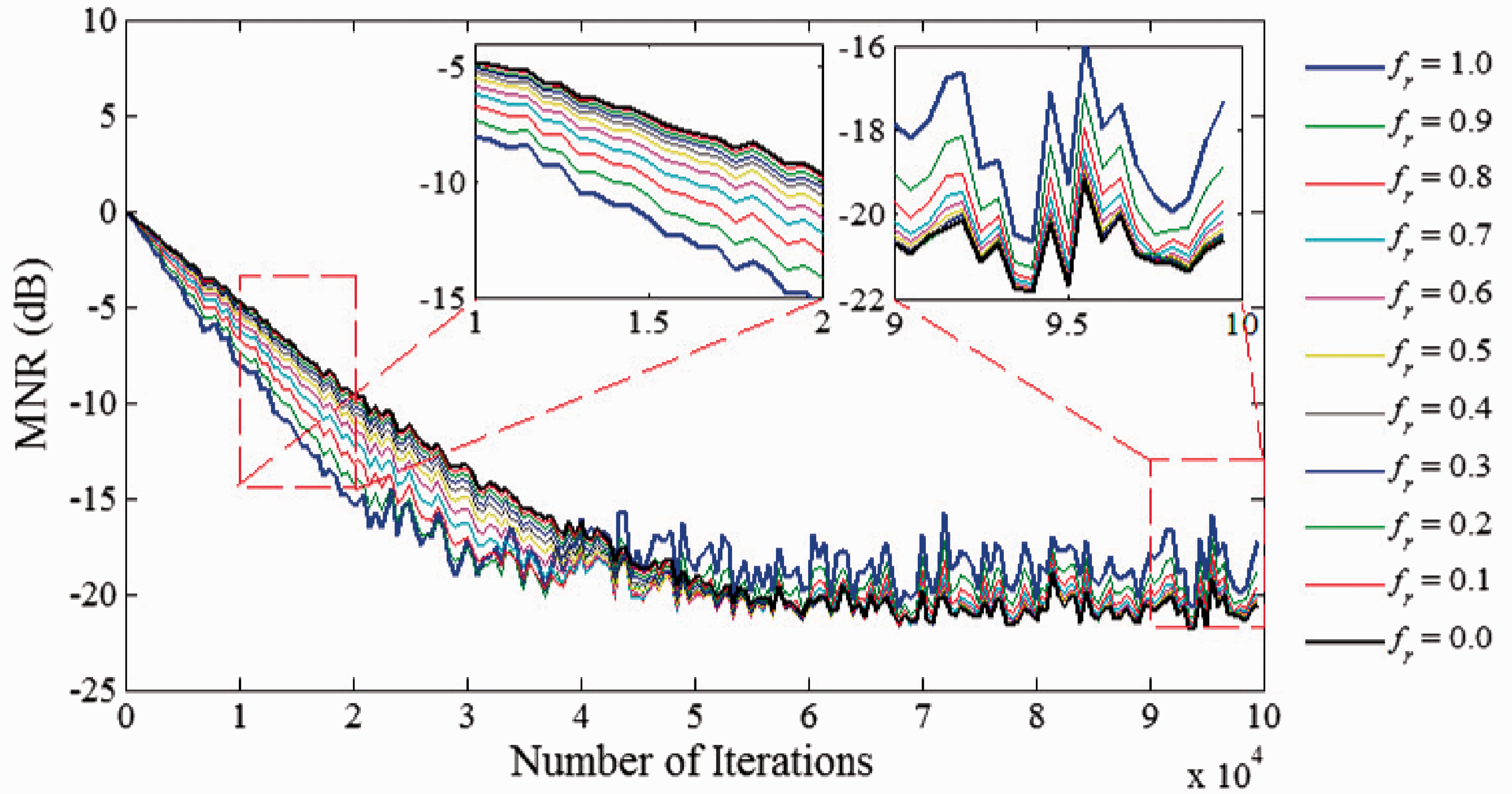
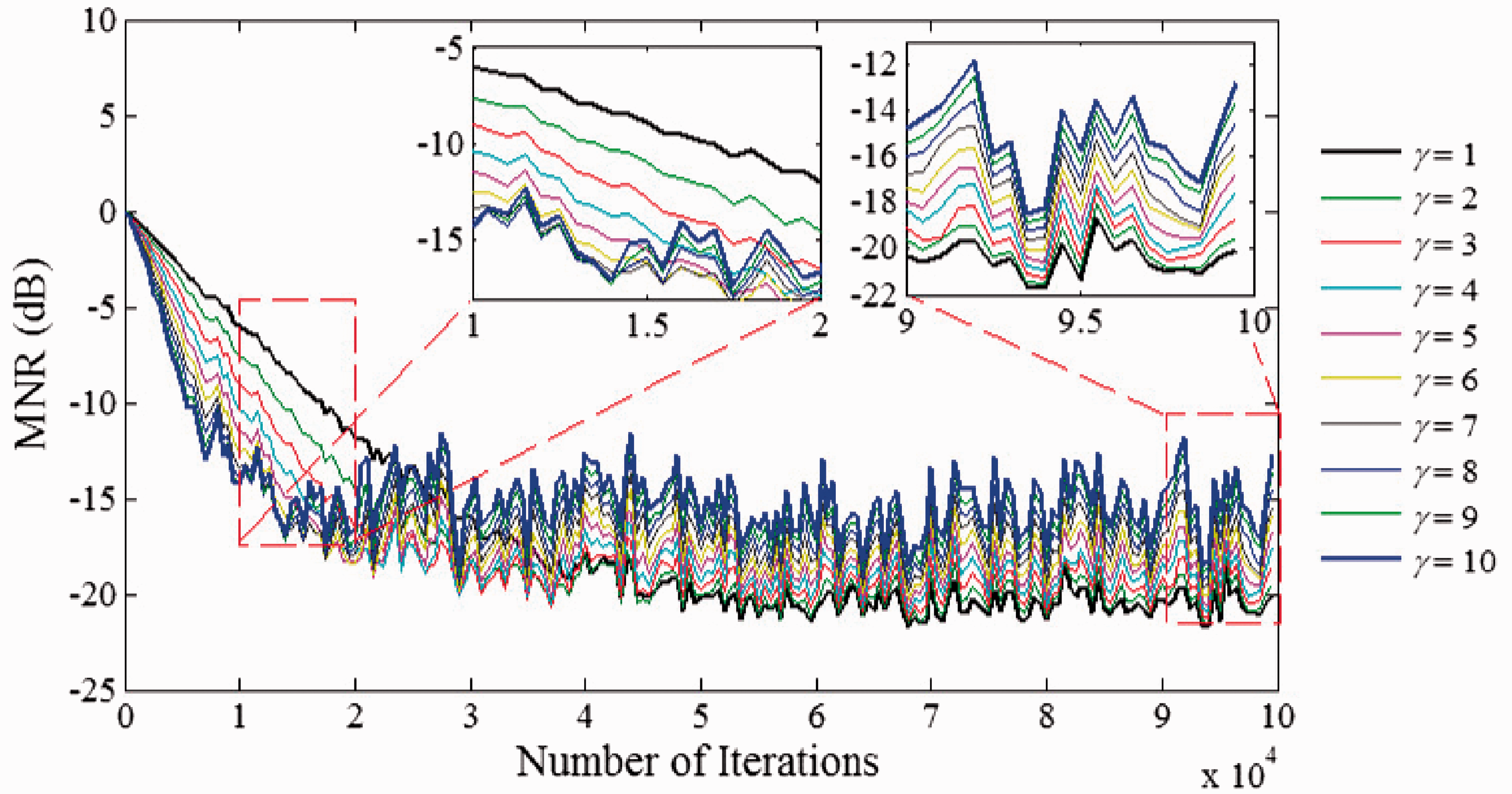
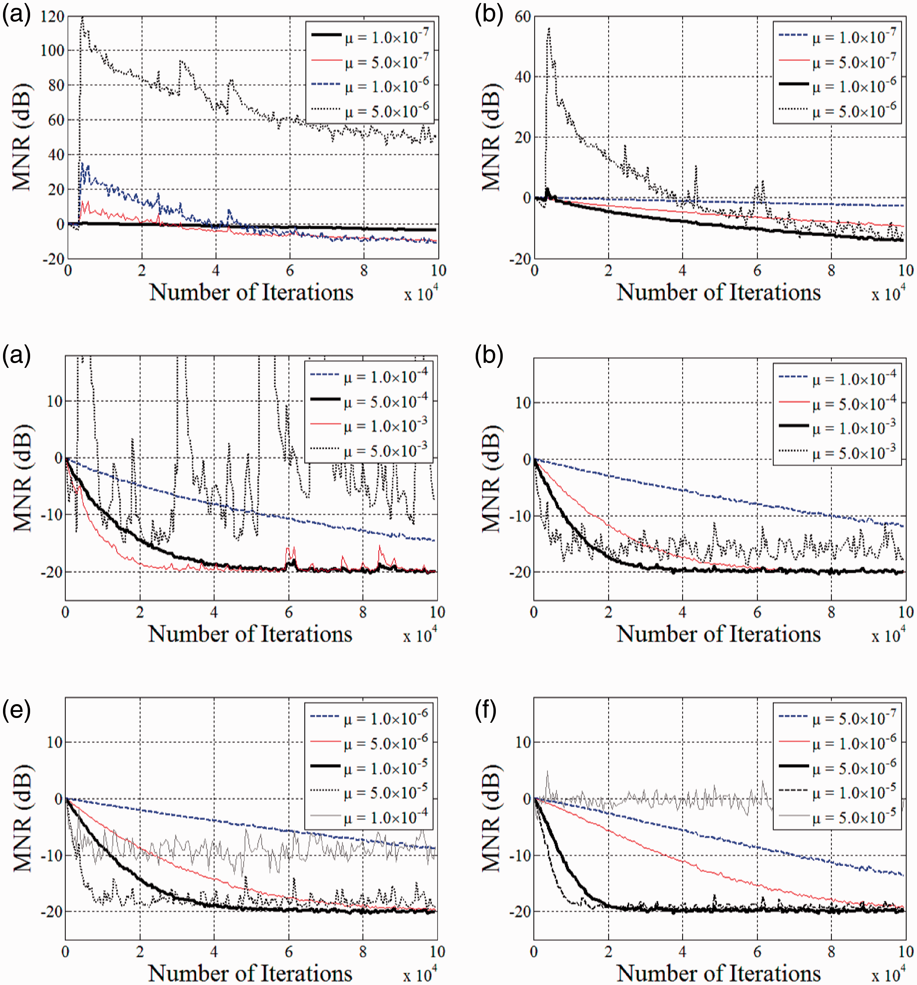
(20) where $E\{·\}$ denotes ensemble averaging and ${\sigma }_e(n)$ and ${\sigma }_d(n)$ are, respectively, estimates for the absolute values of the error signal e(n) and the disturbance signal d(n). Figure 4 shows butterfly plots for MNR performance of the proposed algorithm for variation in the value of the fractional order f_r (the rest of the simulation parameters are given in the caption of Figure 4). We observe that the steady-state noise reduction performance improves for $f_r<1.0$ , however, with some degradation in the convergence speed. We empirically selected the fractional order as $f_r=0.65$ , such that some advantages on the steady-state performance can be gained without too much loss in the convergence speed. The effect of the scaling factor δ, which controls the contribution of the fractional gradient-based term as compared with the ordinary gradient-based term, see equation (19), on the MNR performance of the proposed algorithm is shown in Figure 5 (the rest of the simulation parameters are given in the caption of Figure 5). We observe that $\delta >1$ does improve the convergence speed of the proposed algorithm, however, with some degradation in the steady-state performance. Thus, there is a trade-off situation. We empirically selected $\delta =2.5$ so that an improved convergence speed can be obtained without too much loss in the steady-state performance.

Figure 4.

Effect of the fractional order f_r on the mean noise reduction (MNR) performance of the proposed algorithm ( $\alpha =1.19,\mu =5.0\times {10}^{-7},\delta =1.0$ ).

Figure 5.

Effect of the scaling factor δ on the mean noise reduction (MNR) performance of the proposed algorithm ( $\alpha =1.19,\mu =5.0\times {10}^{-7},f_r=0.65$ ).

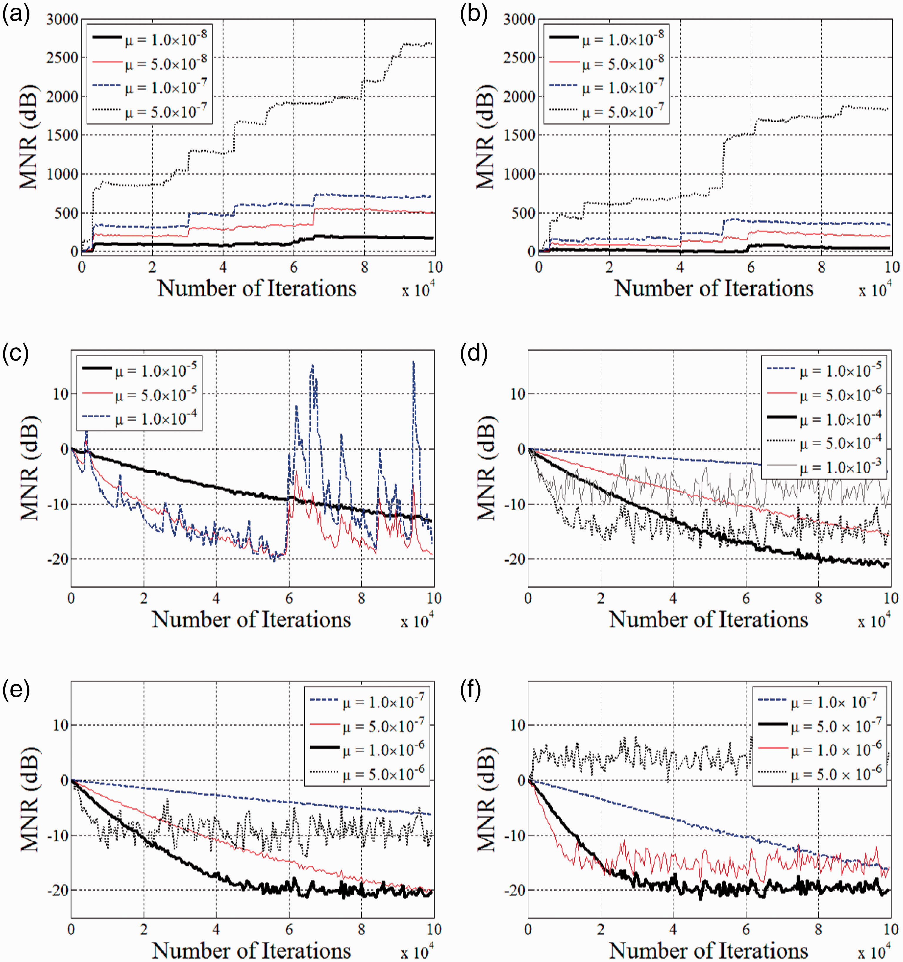
One may argue that the standard normalized step-size (NSS)-based FxLMS (NSS-FxLMS) algorithm ^b may work fine for IANC. In the simulation results presented below, we consider standard NSS-FxLMS algorithm, as well as a modified version equipped with saturation non-linearity-based thresholding of reference and error signals (hereafter referred as NSS-Th-FxLMS algorithm ^c ). Figure 6 shows the simulation results for effect of step-size parameter on the convergence of algorithms discussed in this paper, and Figure 7 presents the performance comparison on the basis of best results in Figure 6. From these simulation results for IANC of strongly impulsive noise sources (being modeled as a standard SαS process with $\alpha =1.19$ ), we make the following observations.

The performance of the FxLMS algorithm (equation (7)) is very poor and is not stable even for a very small step-size. The FxLMS algorithm is derived by minimizing the second order moment, which in fact does not exist for stable processes. Hence, the FxLMS algorithm is not well suited for IANC systems and becomes unstable.

The Sun’s modified FxLMS algorithm (equations (7), (10), (11)) does not give stable performance. As stated earlier, The Sun’s algorithm ignores the peaky samples in the input and does not effectively update the corresponding coefficients of the control filter. This improves the robustness as compared with the FxLMS algorithm (see slow divergence trend in Figure 6(b) as compared with trends in Figure 6(a)); however, the algorithm is never able to converge to a solution good enough to maintain the stability for strongly impulsive sources as considered in the present experiment.

The convergence of the standard NSS-FxLMS is very slow. Since the step-size is normalized with power of the reference signal – peaky signal results in a very small value for the effective step-size, and hence the convergence speed is very slow.

The modified NSS-Th-FxLMS algorithm shows better convergence and steady-state MNR performance, in comparison with NSS-FxLMS algorithm.

In comparison with FxLMS algorithm, the modified-FxLMS-based previous algorithm allows selection of a large value for the step-size parameter (thanks to thresholding of the reference and error signals) and shows good convergence performance.

The performance comparison (on the basis of fast and stable results in Figure 6) is presented in Figure 7, which shows that the proposed algorithm clearly outperforms the rest of algorithms discussed in this paper.

Figure 6.

MNR (in dB) results for (a) standard FxLMS algorithm, (b) Sun’s modified-FxLMS algorithm, (c) standard NSS-FxLMS algorithm, (d) NSS Thresholding FxLMS algorithm, (e) the previous algorithm, and (f) the proposed algorithm, for strongly impulsive noise with $\alpha =1.19$ .

Figure 7.

Performance comparison of standard SαS process with $\alpha =1.19$ (strongly impulsive noise sources). (NSS-FxLMS algorithm: $\mu =1.0\times {10}^{-5}$ , NSS Thresholding FxLMS algorithm: $\mu =1.0\times {10}^{-4}$ , previous algorithm: $\mu =1.0\times {10}^{-6}$ , proposed algorithm: $\mu =5.0\times {10}^{-7}$ .)

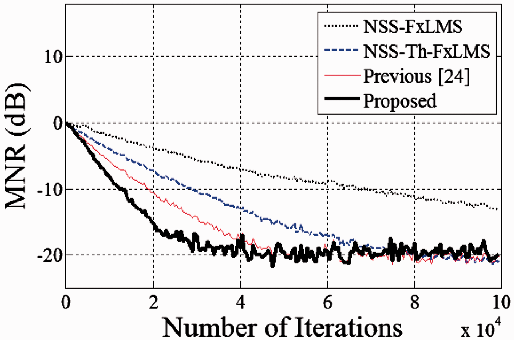
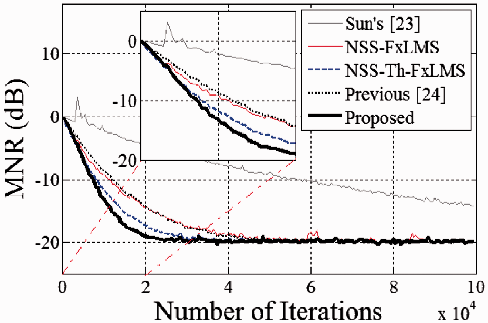
In the second experiment, the reference signal is modeled by standard SαS process with $\alpha =1.79$ . The thresholding parameters $[c_1,c_2]$ are selected in a similar fashion as for $\alpha =1.19$ . The rest of the simulation parameters are also selected to the same values as found previously for $\alpha =1.19$ . The detailed simulation results for studying effect of step-size parameter are shown in Figure 8, and the performance comparison (on the basis of best results in Figure 8) is shown in Figure 9. We observe that the convergence speed of the FxLMS algorithm is very slow (see Figure 8(a)), and hence is not included in the performance comparison shown in Figure 9. The Sun’s algorithm shows somewhat better performance as compared with the FxLMS algorithm, although the convergence speed is very slow. The NSS-based standard and Th-FxLMS algorithms show good performance, which is due to the fact that the present experiment corresponds to noise source close to Gaussian distribution with impulses occurring rarely. The proposed algorithm shows the best convergence speed among the algorithms considered in this paper, as shown in zoomed plots in Figure 9.

Figure 8.

MNR (in dB) results for (a) standard FxLMS algorithm, (b) Sun’s modified-FxLMS algorithm, (c) standard NSS-FxLMS algorithm, (d) NSS Thresholding FxLMS algorithm, (e) the previous algorithm, and (f) the proposed algorithm, for mildly impulsive noise with $\alpha =1.79$ .

Figure 9.

Performance comparison for standard SαS process with $\alpha =1.79$ (mildly impulsive noise sources). (Sun’s algorithm: $\mu =1.0\times {10}^{-6}$ , (NSS-FxLMS algorithm: $\mu =5.0\times {10}^{-4}$ , NSS thresholding FxLMS algorithm: $\mu =1.0\times {10}^{-3}$ , previous algorithm: $\mu =1.0\times {10}^{-5}$ , proposed algorithm: $\mu =5.0\times {10}^{-6}$ .)

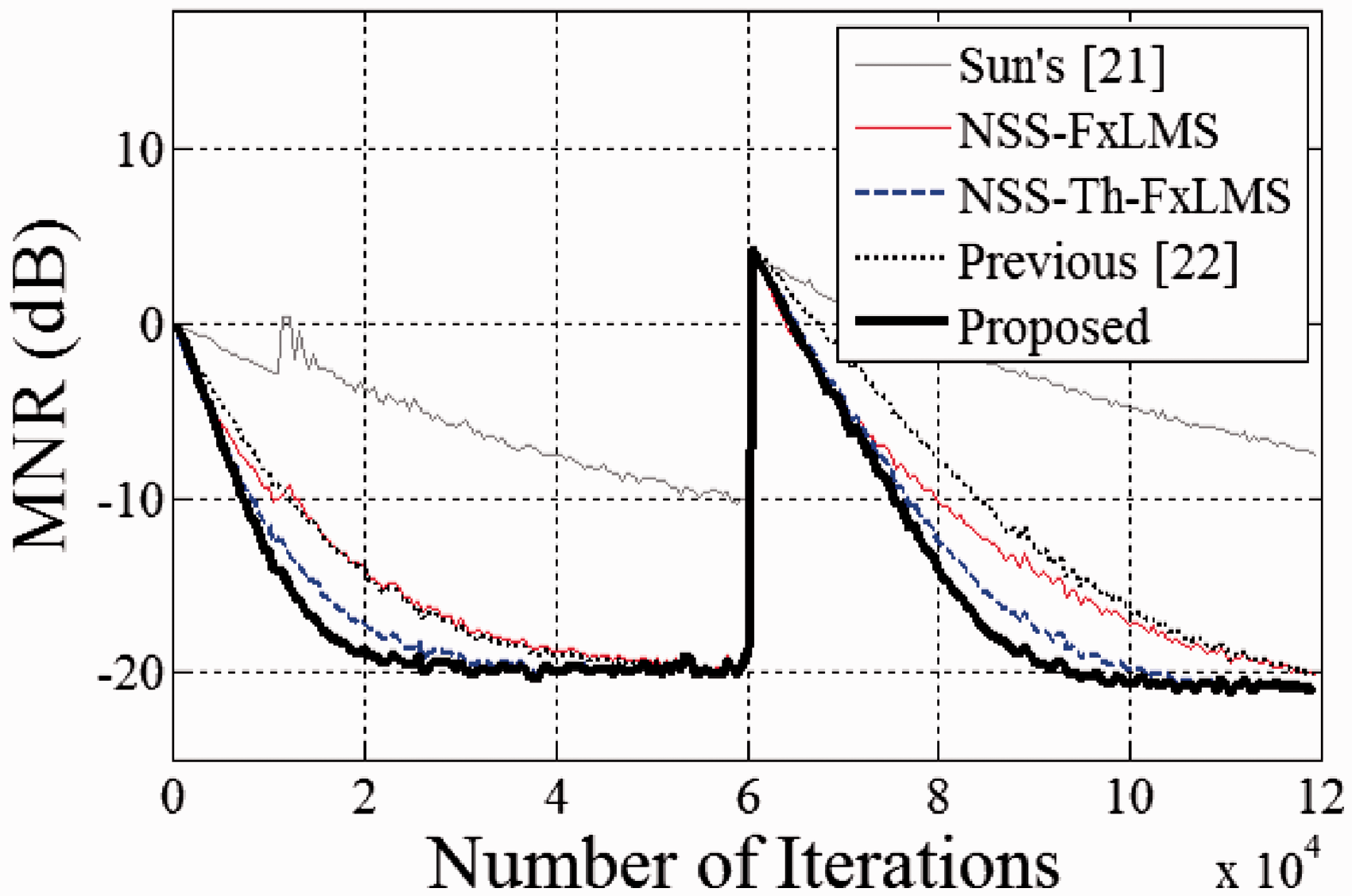
From the above-detailed two experiments, we observe that the proposed method is robust enough against the varying degree of the impulsive nature of the noise source. Further, we investigate the robustness against variations in the acoustic environment. For this purpose, we repeat the experiment for standard SαS process with $\alpha =1.79$ for a sudden change in the acoustic paths P(z) and S(z). At the startup, the acoustic paths have been selected the same as in the previous experiments and suddenly changed to a new ones at the middle of the experiment. The changed acoustic paths have been realized by performing a right circular shift of 2 and 3 samples in the impulse responses of the original P(z) and S(z), respectively. The simulation parameters have been selected to the same values as in the previous experiment for $\alpha =1.79$ , and the simulation results are shown in Figure 10. We observe that the proposed method gives the best performance in comparison with the other methods considered in this paper, before as well as after the sudden change in the acoustic paths.

Figure 10.

Performance comparison for a sudden change in acoustic paths for standard SαS process with $\alpha =1.79$ (mildly impulsive noise sources). (The simulation parameters are same mentioned in caption for Figure 9.)

Concluding remarks

In this paper, we have investigated non-linearity and fractional processing-based adaptive algorithm for IANC systems. The proposed algorithm requires selection of appropriate thresholding parameters $[c_1,c_2]$ , which can be determined by offline analysis. ²⁵ Furthermore, the proposed algorithm requires tuning two empirical constants f_r (the fractional order) and δ (the scaling factor for fractional gradient-based term) (see equation (19)). We have observed that both of these parameters offer a trade-off situation between the convergence speed and steady-state performance. Hence, it is very important to find theoretical bounds for these parameters. It is worth mentioning that in the present literature on IANC systems, simulations are used as a major tool to show the effectiveness of the proposal.^22–24,37 For stable distributions (being used to model the impulsive noise), the second-order moments do not exist. The traditional signal processing techniques based on finite second-order moments may, therefore, not be applicable. ¹⁷ This makes the theoretical analysis very difficult, if not impossible. The theoretical analysis of the proposed algorithm, a very interesting yet a very challenging task, is left as a task for future work. One more direction would be to investigate a data-reusing-type extension of the proposed algorithm as done in Akhtar and Nishihara ³⁸ and Akhtar. ³⁹ It would also be very interesting to design and perform real-time experiments.