H ∞ active control of frequency-varying disturbances in a main engine on the floating raft vibration isolation system

Abstract

Reducing the vibration of marine power machinery can improve warships' capabilities of concealment and reconnaissance. Being one of the most effective means to reduce mechanical vibrations, the active vibration control technology can overcome the poor effect in low frequency of traditional passive vibration isolation. As the vibrations arising from operation of marine power machinery are actually the frequency-varying disturbances, the H_∞ control method is adopted to suppress frequency-varying disturbances. The H_∞ control method can solve the stability problems caused by the uncertainty of the model and reshape the frequency response function of the closed loop system. Two-input two-output continuous transfer function models were identified by using the system identification method and are validated in frequency domain of which all values of best fit exceeds 89%. The method of selecting the weighting functions on the mixed sensitivity problem is studied. Besides, the H_∞ controller is designed for a multiple input multiple output (MIMO) system to suppress the single-frequency-varying disturbance. The numerical simulation results show that the magnitudes of the error signals are reduced by more than 50%, and the amplitudes of the dominant frequencies are attenuated by more than 10 dB. Finally, the single excitation source dual-channel control experiments are conducted on the floating raft isolation system. The experiment results reveal that the root mean square values of the error signals under control have fallen by more 74% than that without control, and the amplitudes of the error signals in the dominant frequencies are attenuated above 13 dB. The experiment results and the numerical simulation results are basically in line, indicating a good vibration isolation effect.

Introduction

The mechanical noise generated by operation of the marine power machinery is the main noise source for warships' underwater radiation, seriously affecting warships' stealth operational performance. By inheriting the floating raft's properties of “mass effect,” “tuning effect,” and “mixed neutralized effect,” ¹ as well as the advantages of the active and passive vibration isolation technology, the active floating raft vibration isolation technology is an important technical means to reduce mechanical vibrations for warships. ²

Although extensive researches on the active vibration control methods have been carried out at home and abroad, the majority of those methods which are designed to suppress mechanical vibrations of the power equipment belong to the adaptive feed-forward control methods, such as the adaptive feed-forward control method based on least mean square (LMS) algorithm, ³ which is widely used owing to its low computational complexity and good convergence, the adaptive feed-forward control method based on neural networks. ⁴ As a highly nonlinear system, neural network has a very strong self-learning ability and can be combined with other algorithms to form a new controller that can achieve an uncertain or unknown system of effective control. However, this requires a lot of parameters and greatly affects the acceptability of the control effect. Harmonic control method ⁵ and the adaptive feed-forward control method based on recursive least square algorithm, ⁶ which has large steady-state error although it converges faster than LMS algorithm. These control algorithms utilize the reference signals and the error signals to adjust the controller parameters according to corresponding updating formulas in the control process, before calculating and outputting a control signal to achieve the purpose of active vibration control. However, these control methods are subject to a common assumption that the disturbance signal is periodic disturbance by default, whose frequency is fixed. In practice, the speed of marine engine is not constant, but fluctuating within a certain range, which leads to frequency fluctuation of the vibration signal within a certain range. ⁷ The existing active vibration control methods which are designed to suppress the periodic disturbances work well, but further researches are required to verify if they do well in frequency-varying disturbances. When the reference signal frequency component of the system is complex and has perturbation, the adaptive feed-forward control method cannot obtain obvious control effect.

Many active control methods are adopted to suppress frequency-varying disturbances abroad. Ballesteros and Bohn ⁸ designed a discrete-time H_∞ optimal gain-scheduling controller to reject harmonic disturbances with time-varying and known frequencies, which was experimentally validated on an active vibration control test bench. Experimental results showed that the controller could suppress a disturbance consisting of six independent harmonics with frequencies that varied within 20 Hz. In terms of the harmonic disturbance with frequency fluctuation, Duarte et al. ⁹ measured the frequencies of time-varying harmonic disturbances directly from the DC motors, designed a corresponding linear parameter varying (LPV) discrete-time controller, and finally carried out experiments on the lightweight elastic structure. Karimi and Emedi ¹⁰ designed a H_∞ gain-scheduled controller for rejection of time-fluctuating narrow-band disturbances and experiments were conducted on the active vibration control system. Airimitoaie and Landau ¹¹ combined the adaptive feed-forward control with feedback control for attenuation of multiple unknown time-varying narrowband disturbances, and real-time experimental results were provided. Landau et al. ¹² used nondirect adaptive control method to reduce the harmonic disturbances with frequency fluctuation and compared with the direct adaptive algorithm based on endometrial principle. The two algorithms were finally verified by experiment. For the narrowband disturbance rejection problem of helicopter tail, Connolly et al. ¹³ compared the LQG control algorithm with the H_∞ control algorithm, and the experimental results showed better performance of the H_∞ control method. Orivuori et al. ⁷ proposed an adaptive LQ feedback control method with frequency estimator to eliminate frequency-varying disturbances on the diesel engine, and three inputs three outputs active vibration control experiments were conducted on a floating raft system.

The majority of active control methods for purpose of suppressing frequency-varying disturbances belong to the feedback control methods, which are mainly applied in structural vibration control field^8,12 and power machinery's vibration control field.^7,13 In the structural vibration control field, the variation range of disturbance signal's frequency is mostly above 5 Hz, and the control methods generally comprise frequency estimator. Thus, these methods use LPV technology to update controller parameters according to the estimated frequency in real time, thereby suppressing the frequency-varying disturbances. As the variation range of disturbance signal's frequency produced by the diesel engine in a warship is small, which is probably less than 1 Hz, ⁷ such disturbances can be suppressed effectively with conventional feedback control methods which require no frequency estimator. LQ control method, ⁷ LQR control method, and H_∞ control method ¹³ belong to the feedback control method, which can suppress disturbances whose frequency varies in a small range. To design a controller, these feedback control methods require an appropriate mathematical model of the controlled object, which should be able to accurately describe the dynamic characteristics of the controlled object.

However, due to the nonlinearity of system, modeling error, and parameter perturbation, the mathematical model is usually slightly different from the actual controlled object, which may lead to overflow instability for a feedback control method. ¹⁴ As the H_∞ control method can describe the difference between the model and the actual controlled object through additive uncertainty and multiplicative uncertainty, the controller based on the H_∞ control method is robust enough to effectively solve the problem of overflow instability. Meanwhile, the H_∞ control method can reshape frequency response function of the closed loop system by shaping design method based on the mixed sensitivity problem, and the designed closed-loop system can effectively suppress frequency-varying disturbances. Thus, the H_∞ control method is utilized to suppress frequency-varying disturbances generated from operation of power machinery.

Modeling of control channel for the floating raft vibration isolation system

Introduction of the floating raft vibration isolation platform

The active floating raft vibration isolation system is composed of two parts, namely mechanical device and electronic control device. As shown in Figure 1, the mechanical device is mainly made up of excitation motors, upper isolators, floating raft, lower isolators, displacement restrictors, electromagnetic actuators, supporting frames, and base. Four excitation motors are fixed above the floating raft as sources of disturbance, which can produce frequency-varying disturbance when operating. The floating raft is connected with the base by four lower rubber isolators, and four electromagnetic actuators and the base are rigidly connected together. The electric control device consists of acceleration sensors, conditioning amplifier, low-pass filter, and data acquisition instrument with signal source, power amplifiers, and dSPACE1103 system. The acceleration signals collected by the acceleration sensors go through the conditioning amplifier and low-pass filter, and then output voltage signals which are directly proportional to the acceleration signals and collected by A/D ports of the dSPACE1103 system to output control signals through D/A ports. After the control signals are enlarged by power amplifiers to drive the electromagnetic actuator, the electromagnetic actuators output corresponding control forces to offset the frequency-varying disturbances generated by the motors.

Figure 1.

Mechanical device of the floating raft vibration isolation system. (a) Front view of the floating raft vibration isolation system and (b) top view of the floating raft vibration isolation system.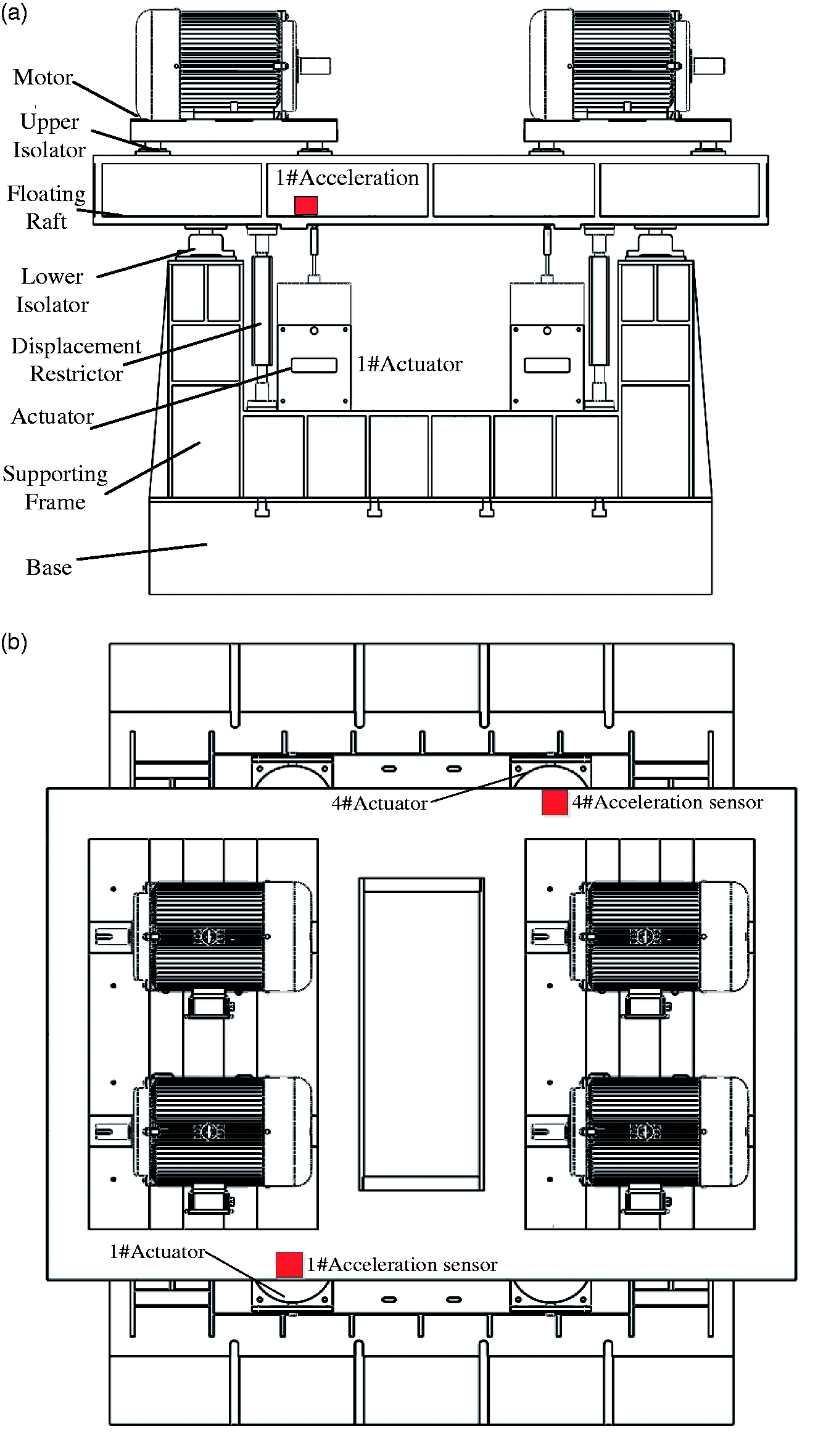

Model identification of control channel for the floating raft vibration isolation system

The floating raft vibration isolation system is a typical nonlinear and strong coupling system, whose internal mechanism is not clear. Thus, it is not suitable for analysis modeling. Floating raft vibration isolation system generally has multiple units and can produce different perturbation and disturbance frequency. As the unit and the unit, and the unit and the raft are mutually coupled and interacted, floating raft isolation system is a multidisturbance source and multidirectional vibration isolation system. In a floating raft vibration isolation system, as multiple units need installing on the same raft, which will result in a complex structure of the raft, the raft cannot be simply considered as a rigid body. The system identification method only calls for input and output data of the controlled object with no need to understand the internal mechanism of the controlled object. In addition, this method can also accurately describe the dynamic characteristics of the controlled object, so it is used to establish the mathematical model of control channel for the floating raft vibration isolation system. The H_∞ control method requires a mathematical model of the controlled object, the function tfest() of System Identification Toolbox on MATLAB can be called to identify an optimal discrete transfer function according to the frequency response of the controlled object. The structural model of the function is output error model, and the identification algorithm is the prediction error method.

Figure 2 is the schematic of model identification for the floating raft vibration isolation system. The input signal is white noise signal whose frequency range is 0.1–200 Hz and effective value of voltage is 1.5 V. The white noise signal generated from the signal source goes through the low-pass filter and the power amplifier, and then drives the actuator on the floating raft vibration isolation system. The output signal acquired by the acceleration sensor is transmitted to data acquisition instrument after conditioning, amplification, and filtering; the acquired input signal is white noise signal which is filtered. The sampling time is 12.8 s and the sampling frequency is 2560 Hz.

Figure 2.

Schematic of model identification for the floating raft vibration isolation system.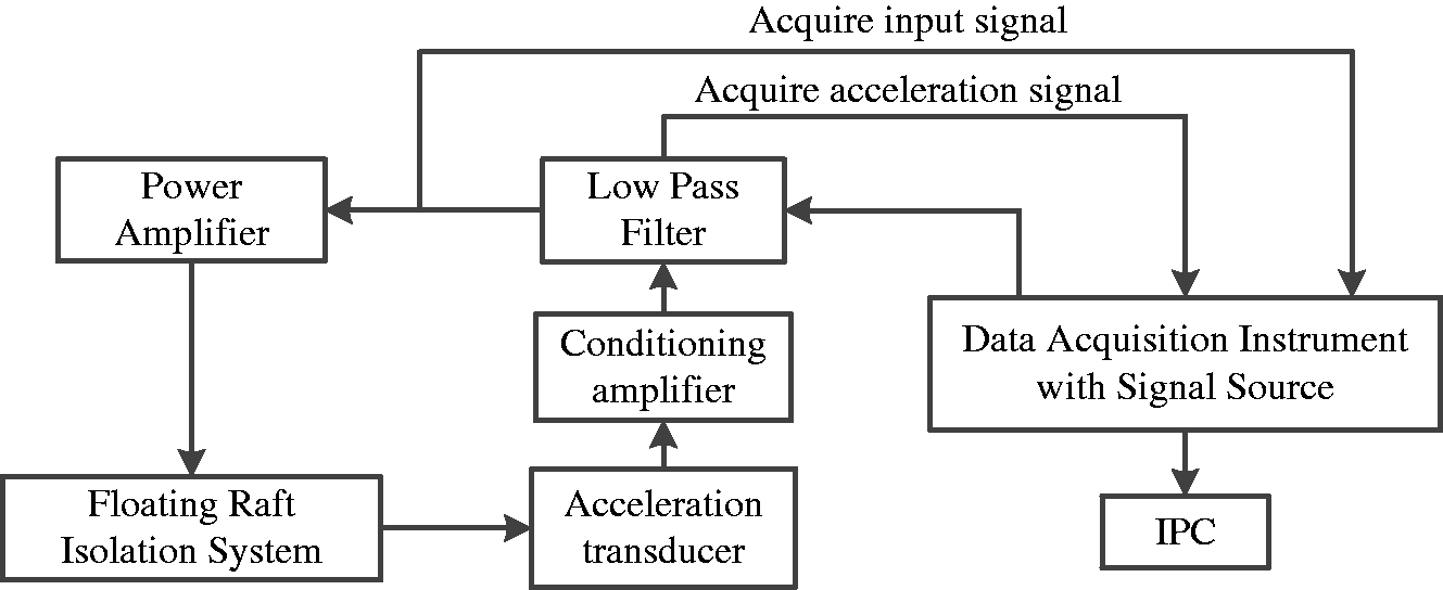

In Figure 1, the 4#actuator and the 4# sensor are placed diagonally relative to the 1#actuator and the 1# sensor, and the corresponding power amplifier's numbers are, respectively, 1# and 4#. G11 represents the transfer function from 1# amplifier to the 1# sensor, G14 represents the transfer function from 1# amplifier to the 4# sensor, G41 represents the transfer function from 4# amplifier to the 1# sensor, and G44 represents the transfer function from 4# amplifier to the 4# sensor. The frequency characteristics of the four control channel are shown in Figure 3 from which it can be seen that the G11 and G44 are similar, and G14 and G41 are almost identical. Since we have chosen the same type of power amplifier and actuator in the system, we have the same frequency response function in theory. And the structure of the floating raft isolation system is symmetrical; the arrangement of the motor is also symmetrical. Therefore, according to the symmetry, the frequency response function of each channel is theoretically the same, the transfer function G11 and G44, G14 and G41 should theoretically be approximately identical. The theoretical results can be well validated by the experimental data.

Figure 3.

Frequency characteristic of the control channels.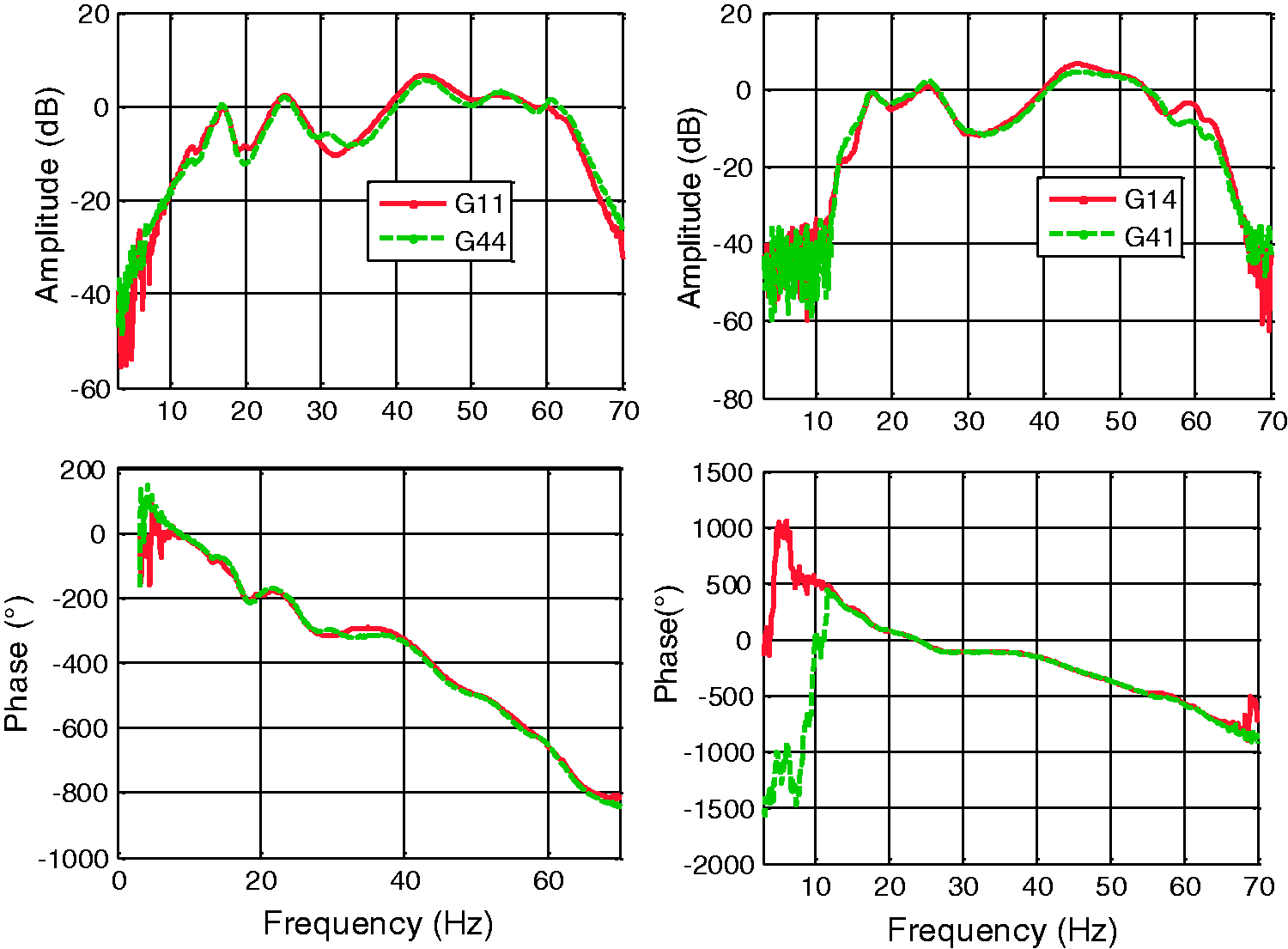

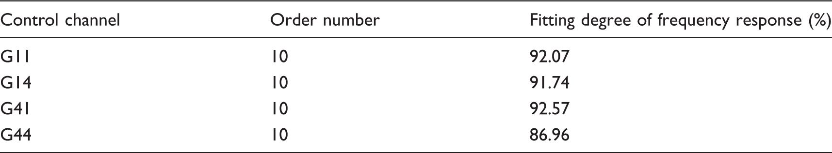
The function d2c () in MATLAB can be called to transform the identified discrete transfer functions into the desired continuous transfer functions. The G11, G14, G41, and G44 control channel models' orders are 10, and the identified models' goodness of fitness with the experimental data in the frequency domain is, respectively, 92.07, 91.74, 92.57, and 86.96%. The four control channel models' poles are located in the left side of the complex plane, which indicates stable models performance. As the identified models are processed by model verification, they can accurately describe the dynamic characteristics of the controlled object.

As shown in Figure 3, the degree of curve fitting is generally high, but at low frequencies, especially 0–15 Hz frequency is relatively low degree of fit, which is mainly due to two reasons. First, the frequency response of the power amplifier and actuator is relatively poor in the low frequency, and second, there is a certain standing wave effect in passive vibration isolator. The wider the frequency characteristic analysis of the controlled object, the richer the dynamic characteristics of the controlled object, which requires a higher order of mathematical model to accurately describe the dynamic characteristics of the controlled object, however, higher order of mathematical model makes it more difficult to design and analyze the control system. According to the frequency range of the disturbance signal and the design performance requirements of the control system, this paper chooses to analyze the frequency characteristics of the controlled object in the frequency range of 0–60 Hz. Because the vibration that needs to be suppressed is the vibration of the ship's power machine, the main frequency components of the vibration signal are in the range of 10–50 Hz, so the result of the system model identification meets the actual requirements.

The identified model also needs to be modeled to determine whether it can accurately describe the dynamic characteristics of the controlled object. The model verification mainly examines the fitting degree of the model. The fitting degree of the model means the fitting degree between the model data and the experimental data. It shows the fitting degree between the model frequency response and experimental frequency response of the four control channel in Figure 4. It can be seen from Figure 4, the fitting degree in the frequency range of 15–65 Hz is very high, and the frequency response error of each channel is within 0.3.

Figure 4.

Model and experimental data fitting degree of each control channel. (a) Control channel G11, (b) control channel G14, (c) control channel G41, and (d) control channel G44.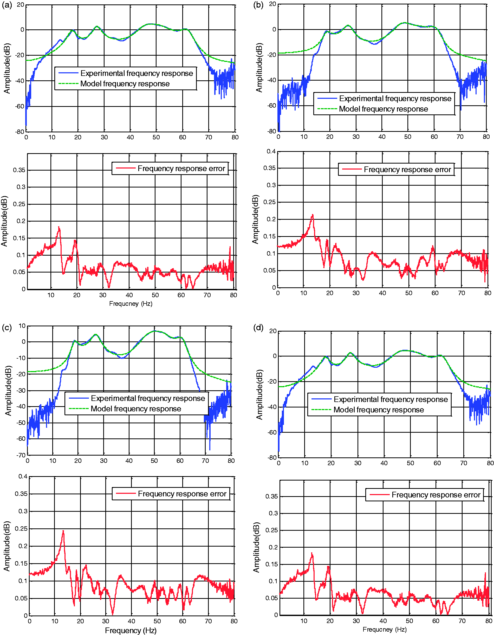

The frequency response is the evaluation index of the system identification toolbox. The order and the fitting degree of each control channel model are shown in Table 1. In Table 1, the order of each control channel model is 10 orders, which can meet the requirements of the model on the order, and the fitting degree is more than 85%, which indicates a high degree of fit between the model and the experimental data. The model can accurately describe dynamic characteristics of the controlled object in frequency range of 15–65 Hz.

Table 1.

Fitting degree of frequency response and order number.

Control channel	Order number	Fitting degree of frequency response (%)
G11	10	92.07
G14	10	91.74
G41	10	92.57
G44	10	86.96

The expressions of the continuous transfer functions for each control channel are shown in Appendix 1.

H_∞ control theory of the floating raft vibration isolation system

The feedback control method can effectively suppress the frequency-varying disturbance, and the block diagram of feedback control is shown in Figure 5. The error signal e produced by the superposition of the disturbance signal d and the desired output signal y is detected and sent to the controller K (s); the controller calculates and outputs a control signal u according to the control law, and the control signal u goes through the control channel G (s) before generating the desired output signal y ; the desired output signal and the disturbance signal cancel each other out to eliminate the frequency-varying disturbance.

Figure 5.

Block diagram of feedback control for suppressing frequency-varying disturbance.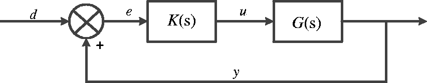

In case there is external disturbance force but without actuator control, the sensor measures the error signal e that is equal to the disturbance signal d . When the actuator controls but external disturbance force is absent, the sensor measures the error signal e that is equal to the desired output signal y .

Uncertainty of the model and its description

In the floating raft isolation system, due to the vibration isolators' nonlinearity, the raft's flexibility, the parameter perturbation, unmodeled dynamics in high frequency, and the system identification error, it is difficult to establish a precise mathematical model. The difference between the mathematical model and the actual controlled object must be taken into consideration when designing the control system, so that the designed controller based on an error model can still guarantee the actual closed-loop system's stability, achieving the desired designing goals. The difference between the mathematical model and the controlled object is called as model uncertainty, and the common description methods for model uncertainty are addition uncertainty description and multiplication uncertainty description, respectively, as shown in equations (1) and (2) ¹⁵

$$\tilde{G}(s)-G(s)=\Delta (s)*W_2(s)$$

(1)

$$\frac{\tilde{G}(s)-G(s)}{G(s)}=\Delta (s)*W_3(s)$$

(2)

where $\tilde{G}(s)$ is the actual controlled object, $G(s)$ is the nominal model, $\Delta (s)$ is the uncertainty after normalized, $W_2(s)$ represents the addition uncertainty of model, and $W_3(s)$ represents the multiplication uncertainty of model.

Mixed sensitivity problem

When designing the control system, it is necessary to not only consider the robust stability requirement of the closed-loop control system due to the differences between the mathematical model and the actual controlled object, but also take into account the performance requirement of the control system. The mixed sensitivity problem is a typical designing problem for the H∞ controller, which can transform both requirements into the optimization problem of the H_∞ norm ¹⁶ when designing a control system. A typical block diagram of the mixed sensitivity problem is shown in Figure 5. Where, G is the nominal model, K is the controller to be designed, W ₁, W ₂, and W ₃ are three different weighting functions; w is the input signal; z₁, z₂, and z₃ are the weighted outputs; y is the error signal measured by sensor; u is the control signal output from the controller. The area surrounded by the dashed box is augmented controlled object, including the controlled object G and three weighting functions.

The mixed sensitivity problem can be understood as selecting three appropriate weighting functions and solving a controller 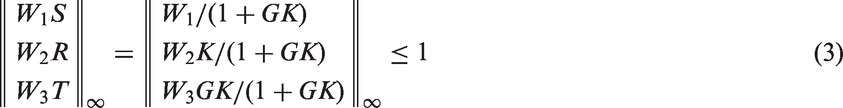K to make the system meet the robust stability and performance requirements, namely the controller K enables the establishment of formula (3)

$$\begin{array}{c}\multicolumn{1}{c}{\Vert \begin{array}{c}{W}_{1}S\\ W_{2}R\\ W_{3}T\end{array}{\Vert }_{\infty }=\Vert \begin{array}{c}{W}_1/(1+\mathit{GK})\\ W_{2}K/(1+\mathit{GK})\\ W_3\mathit{GK}/(1+\mathit{GK})\end{array}{\Vert }_{\infty }\le 1}\end{array}$$

(3)

S is the sensitivity function, T is the complementary sensitivity function, R is the controller sensitivity function. Where, $\Vert W_{1}S{\Vert }_{\infty }\le 1$ represents the performance requirements, $\Vert W_{2}R{\Vert }_{\infty }\le 1$ & $\Vert W_{3}T{\Vert }_{\infty }\le 1$ both represent the robust stability requirements.

Selection of the weighting function

The solution of mixed sensitivity problem needs to be converted into a standard H_∞ control problem. Doyle et al. ¹⁷ offers a classic DGKF which is also called as the Algebraic Riccati equation RIC method to solve the standard H_∞ control problem and a central controller is designed by solving Riccati equations in this method. In order to solve mixed sensitivity problem requires three appropriate weighting functions W₁, W₂, and W₃ should be selected in advance, because the quality of these three weighting functions can directly affect the designed controller's capacity to meet the designing requirements. Currently, there have yet not been mature rules to select the weighting function, and cut-and-try method is mostly used. When designing the control system, first select the weighting function W₂ and W₃, followed by selection of the weighting function W₁. The weighting function W₂ and W₃ are related to model uncertainties, including the absolute error and the relative error between the model response and the experimental frequency response. The weighting function W₁ should be selected according to the frequency characteristics of external interference. In order to suppress the frequency-varying disturbance, whose dominant frequency ranges from 1 Hz, the amplitude of the performance-related sensitivity function S in dominant frequency must be less than 1. For the single-input single-output system, the system performance requirement can be described by equation (4)

$$\Vert W_{1}S{\Vert }_{\infty }\le 1\Rightarrow |S(\mathit{jw})|\le |{W_1}^{-1}(\mathit{jw})|$$

(4)

Equation (4) shows that as the sensitivity function S 's frequency characteristic $|S(\mathit{jw})|$ must be located below the $|{W_1}^{-1}(\mathit{jw})|$ , the amplitude of $|W_1(\mathit{jw})|$ in dominant frequency must be larger than 1. It can make the $|W_1(\mathit{jw})|$ present a peak shape in dominant frequency, thus the $|S(\mathit{jw})|$ and the $|{W_1}^{-1}(\mathit{jw})|$ manifest themselves as a null in dominant frequency, which indicates that the entire feedback control system can highly suppress the disturbance signal containing the dominant frequency component.

If only a dominant frequency is to be suppressed, W ₁ can be selected as a single peak shape with the peak value located at the dominant frequency, as shown in formula (5) and (6)

$$W_1=k\frac{s}{s^2+2\xi \mathit{ws}+w^2}$$

(5)

$$w_d=w\sqrt{1-{\xi }^2}$$

(6)

In equations (5) and (6), $w_d$ is the dominant frequency which needs suppressing; k and ξ are regarded as adjustment parameters when selecting W ₁.

For a MIMO control system, if there is only a frequency-varying disturbances containing a dominant frequency component that needs suppressing, the selection method for weighting functions is as the same as the SISO control system, except that those three weighting functions need to become a corresponding diagonal matrix.

H_∞ controller designed for a MIMO control system

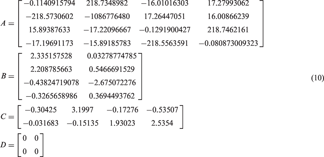
The W ₂ is chosen to describe the model uncertainty and its value is determined by the absolute error between the model frequency response and the experimental frequency response. The four identified channels' model frequency responses and experimental frequency responses are limited from 0 to 60 Hz, and the absolute error are all less than 0.2. In order not to increase the order numbers for controllers and to obtain a larger robust stability, the optional weighting function W ₂ is assigned as 0.1 and W ₃ as 0.

The H∞ controller is designed with the following steps:

Adjust the parameters and and tentatively give a weighting function W ₁. By relying on the transfer function of the control channel and the weighting functions W ₁, W ₂, and W ₃, call the hinfsyn () function in the MATLAB software to solve the H∞ controller K. If there is no solution to the mixed sensitivity problem, reduce the parameter k appropriately. After k is reduced, if the mixing sensitivity problem remains unsolved, which may be due to the excessive weighting function W ₂, reduce the amplitude of W ₂ and reexecute step (I).

Verify whether the closed-loop control system is inherently stabile, namely to check whether the designed controller and closed-loop control system are stable. If the control system is not inherently stable, proceed from step I and modify the selection parameters of the weighting function W ₁ appropriately. If the system is inherently stable, proceed to the next step.

Check Bode Plots regarding the sensitivity function of the closed-loop control system to determine whether the system meets the performance requirements. If not, go back to step (I); if yes, end the controller design.

The weighting function W ₁ is selected according to formula (5), and the W ₂ is determined by the dominant frequency of disturbance signal. Assume that a disturbance whose dominant frequency varies close to 30 Hz is to be suppressed and the variation range of frequency is no more than 1 Hz. $w_d$ can be assigned to $2\times \pi \times 30=188.4\text{rad}/\text{s}$ .

According to formula (5) and (6), by conducting a series of spreadsheets, and in order to ensure the stability for the controller 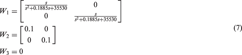K and the closed-loop control system under stable conditions, the weighting functions eventually are identified as

$$\begin{array}{c}\multicolumn{1}{c}{W_1=[\begin{array}{cc}\frac{s}{s^2+0.1885s+35530}& \hfill 0\hfill \\ 0& \hfill \frac{s}{s^2+0.1885s+35530}\hfill \end{array}]}\\ \multicolumn{1}{c}{W_2=[\begin{array}{cc}0.1& \hfill 0\hfill \\ 0& \hfill 0.1\hfill \end{array}]}\\ \multicolumn{1}{c}{W_3=0}\end{array}$$

(7)

The mathematical model of the control channel is a two-input two-output transfer function matrix made up of four channels. According to the mathematical model 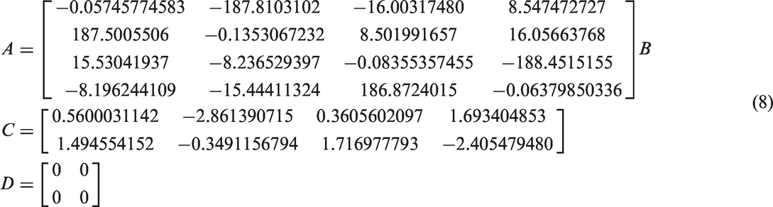G (s) of the control channel, the weighting functions W ₁, W ₂, and W ₃, and the hinfsyn () function in MATLAB can be called to solve the robust controller K . The controller K is a two-input two-output state-space equation, and the dimension of the matrix A is 44. Due to too large controller order, it is not conducive to the control algorithm, and thus the controller order should be reduced. The bstmr () function in MTALB can be used to complete order reduction. Under the condition that there is little change of the dynamic characteristics of the controller K , the dimension of the matrix A is reduced to 4. The state-space expression of the controller after reducing order follows as formula (8)

$$\begin{array}{c}\multicolumn{1}{c}{A=[\begin{array}{cccc}-0.05745774583& \hfill -187.8103102\hfill & \hfill -16.00317480\hfill & \hfill 8.547472727\hfill \\ 187.5005506& \hfill -0.1353067232\hfill & \hfill 8.501991657\hfill & \hfill 16.05663768\hfill \\ 15.53041937& \hfill -8.236529397\hfill & \hfill -0.08355357455\hfill & \hfill -188.4515155\hfill \\ -8.196244109& \hfill -15.44411324\hfill & \hfill 186.8724015\hfill & \hfill -0.06379850336\hfill \end{array}]B=[\begin{array}{cc}2.724889168& \hfill -0.8050106367\hfill \\ -1.590320803& \hfill -0.4766626217\hfill \\ -1.085861943& \hfill -3.082330315\hfill \\ 0.2714032574& \hfill -0.7586295242\hfill \end{array}]}\\ \multicolumn{1}{c}{C=[\begin{array}{cccc}0.5600031142& \hfill -2.861390715\hfill & \hfill 0.3605602097\hfill & \hfill 1.693404853\hfill \\ 1.494554152& \hfill -0.3491156794\hfill & \hfill 1.716977793\hfill & \hfill -2.405479480\hfill \end{array}]}\\ \multicolumn{1}{c}{D=[\begin{array}{cc}0& \hfill 0\hfill \\ 0& \hfill 0\hfill \end{array}]}\end{array}$$

(8)

where A represents the system state matrix, B represents the control input matrix, C represents the system output matrix, and D represents the input and output correlation matrix.

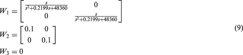
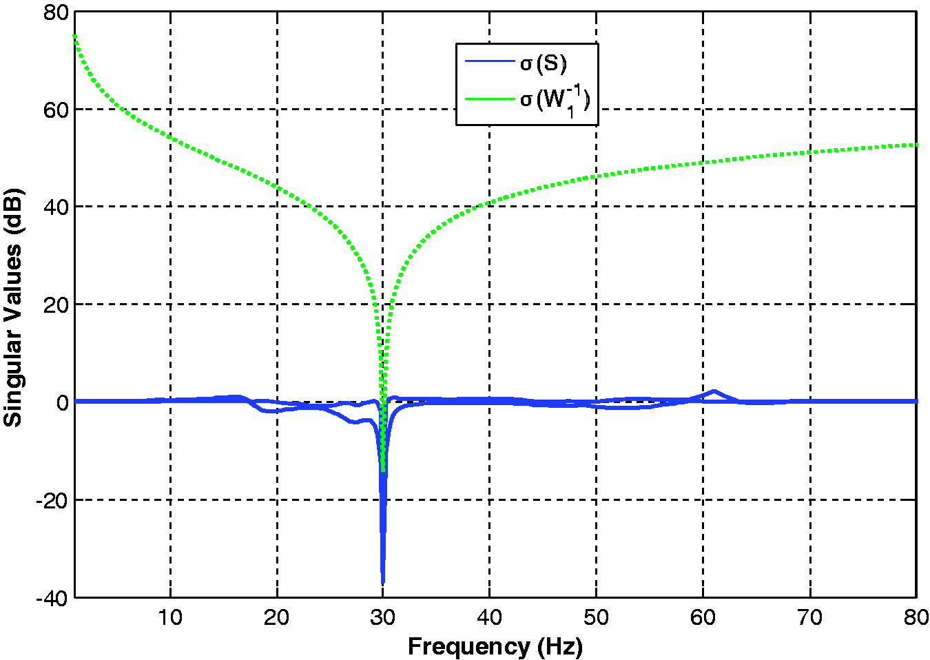
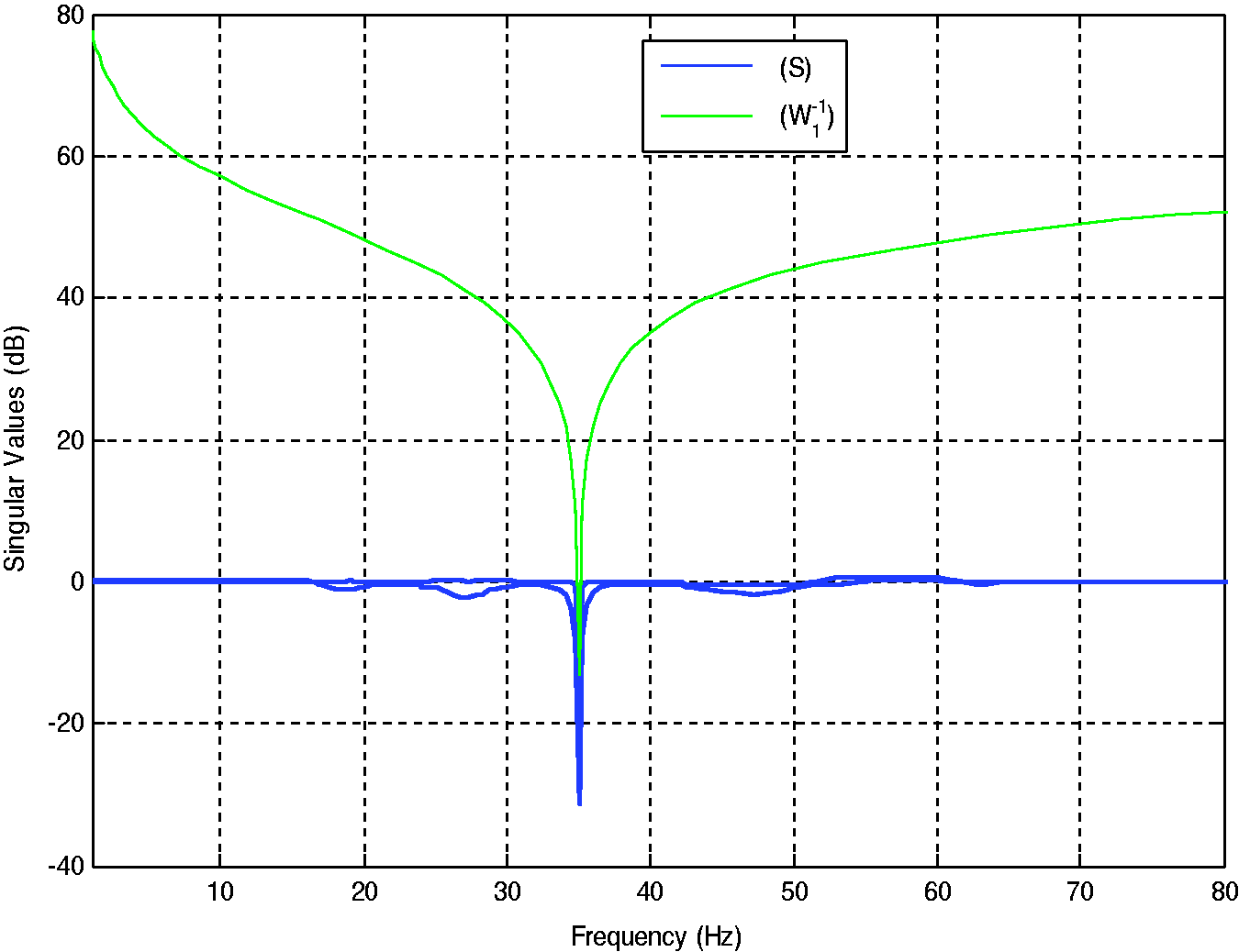
With the same method above, the weighing functions and the controller K can be designed when the disturbance whose dominant frequency varies close to 35 Hz. The weighing functions and the controller K are defined as

$$\begin{array}{c}\multicolumn{1}{c}{W_1=[\begin{array}{cc}\frac{s}{s^2+0.2199s+48360}& \hfill 0\hfill \\ 0& \hfill \frac{s}{s^2+0.2199s+48360}\hfill \end{array}]}\\ \multicolumn{1}{c}{W_2=[\begin{array}{cc}0.1& \hfill 0\hfill \\ 0& \hfill 0.1\hfill \end{array}]}\\ \multicolumn{1}{c}{W_3=0}\end{array}$$

(9)

$$\begin{array}{c}\multicolumn{1}{c}{A=[\begin{array}{cccc}-0.1140915794& \hfill 218.7348982\hfill & \hfill -16.01016303\hfill & \hfill 17.27993062\hfill \\ -218.5730602& \hfill -1086776480\hfill & \hfill 17.26447051\hfill & \hfill 16.00866239\hfill \\ 15.89387633& \hfill -17.22096667\hfill & \hfill -0.1291900427\hfill & \hfill 218.7462161\hfill \\ -17.19691173& \hfill -15.89185783\hfill & \hfill -218.5563591\hfill & \hfill -0.080873009323\hfill \end{array}]}\\ \multicolumn{1}{c}{B=[\begin{array}{cc}2.335157528& \hfill 0.03278774785\hfill \\ 2.208785663& \hfill 0.5466691529\hfill \\ -0.43824719078& \hfill -2.675072276\hfill \\ -0.3265658986& \hfill 0.3694493762\hfill \end{array}]}\\ \multicolumn{1}{c}{C=[\begin{array}{cccc}-0.30425& \hfill 3.1997\hfill & \hfill -0.17276\hfill & \hfill -0.53507\hfill \\ -0.031683& \hfill -0.15135\hfill & \hfill 1.93023\hfill & \hfill 2.5354\hfill \end{array}]}\\ \multicolumn{1}{c}{D=[\begin{array}{cc}0& \hfill 0\hfill \\ 0& \hfill 0\hfill \end{array}]}\end{array}$$

(10)

Upon examination, the designed control system meets the internal stability condition, and the shaping design results based on the mixed sensitivity problem is shown as Figure 6. As shown in Figure 7, there are two curves for the singular value of the sensitivity function S in the closed-loop control system, and the two curves are below the singular value of the function $W_1^{-1}$ , and the singular values of the sensitivity function S and the function $W_1^{-1}$ at the frequency 30 Hz nearby present concave shapes, which indicates that the closed-loop control system can effectively suppress frequency-varying disturbance with dominant frequency of 30 Hz. In Figure 8, we can conclude that control system can effectively suppress frequency-varying disturbance with dominant frequency of 35 Hz in the same way.

Figure 6.

Block diagram of the mixed sensitivity problem.

Figure 7.

Shaping design result for 30 Hz frequency-varying disturbance.

Figure 8.

Shaping design result for 35 Hz frequency-varying disturbance.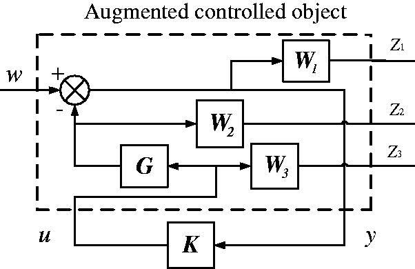

The simulation block diagram for a MIMO feedback control system is shown in Figure 9. Sweep signal is used to simulate frequency-varying disturbance, and the sweep signal 1 and the sweep signal 2 are, respectively, used as the disturbance signal 1 and the disturbance signal 2, of which the duration are both 5 s. To distinguish two disturbance signals, one of sweep signals goes through a gain of 0.8 narrow links.

Figure 9.

Robust control for a MIMO control system. MIMO: multiple input multiple output.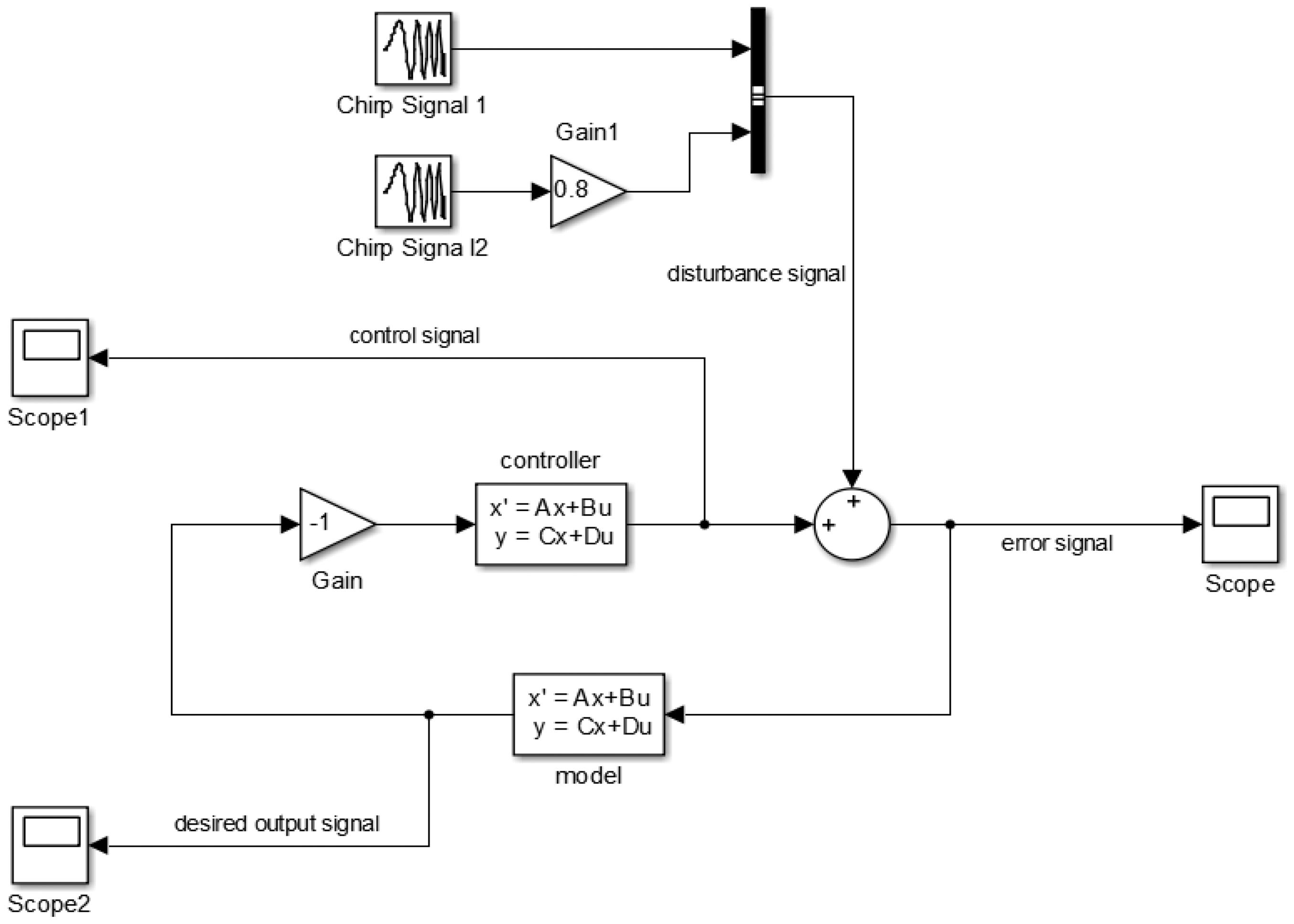

The simulation results are shown in Figure 10, where Figure 10(a) is the time-domain diagram and self-power spectrum for the error signal 1 before and after control, and Figure 10(b) is the time-domain diagram and power spectrum for the error signal 2 before and after control. As it can be seen, the magnitudes of two error signals are reduced by more than 50%, and the amplitudes of the error signal 1 and the error signal 2 in 30 Hz have fallen by about 15 dB. This indicates that the control system can effectively suppress frequency-varying disturbance with dominant frequency of 30 Hz.

Figure 10.

Time-domain diagram and self-power spectrums of the error signals of 30 Hz.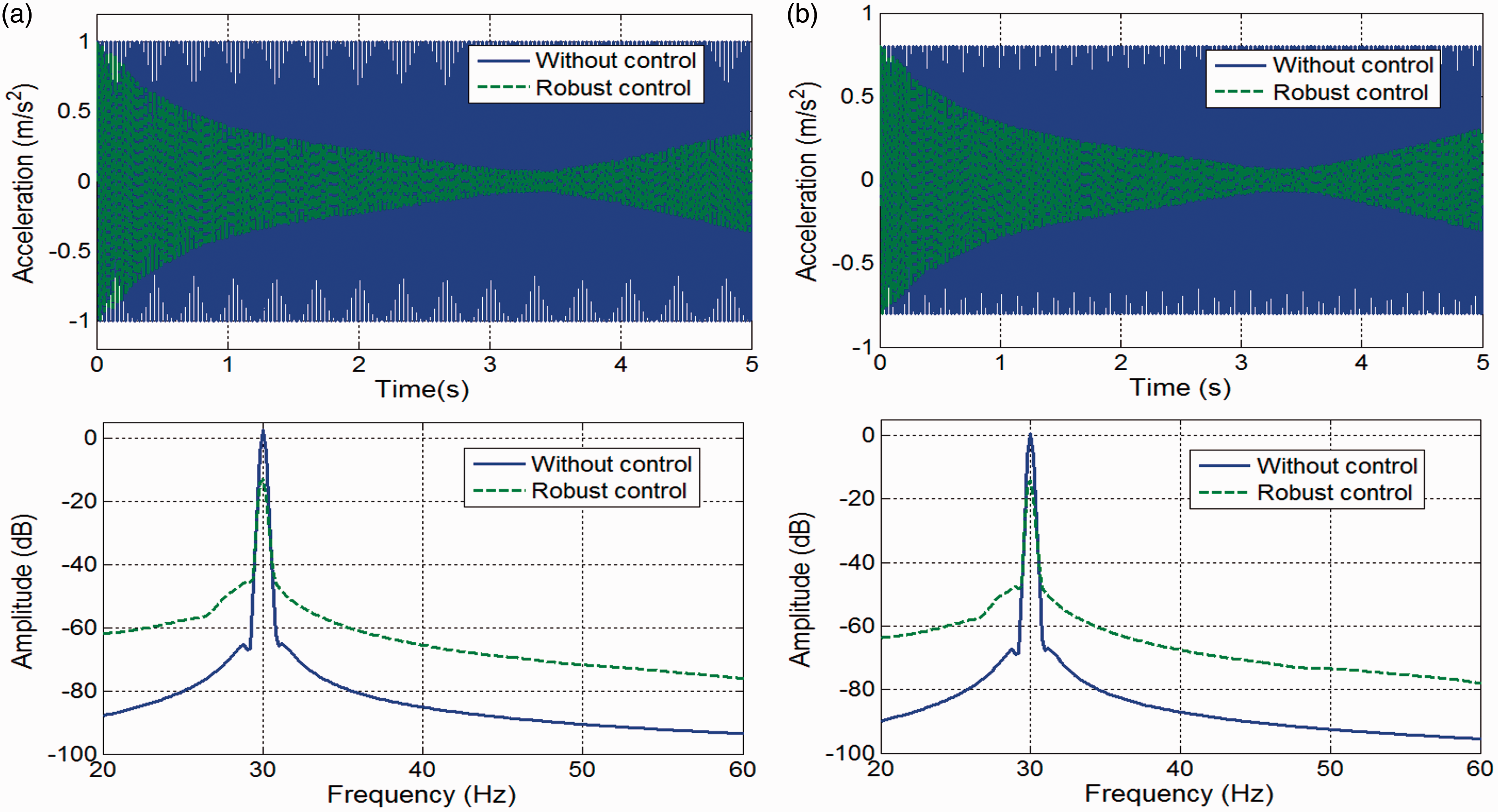

In order to verify universality of the H_∞ controller designing method, another controller is designed for frequency-varying disturbances with dominant frequency of 35 Hz, which is shown in Figure 11. The simulation results show that when the disturbance signal's frequency varies around 35 Hz, the dominant frequency's magnitudes of the error signal 1 and the error signal 2 fall by about 10 dB. It shows that the designed system can effectively suppress frequency-varying disturbance whose dominant frequency varies around 30 and 35 Hz.

Figure 11.

Time-domain diagram and self-power spectrums of the error signals of 35 Hz.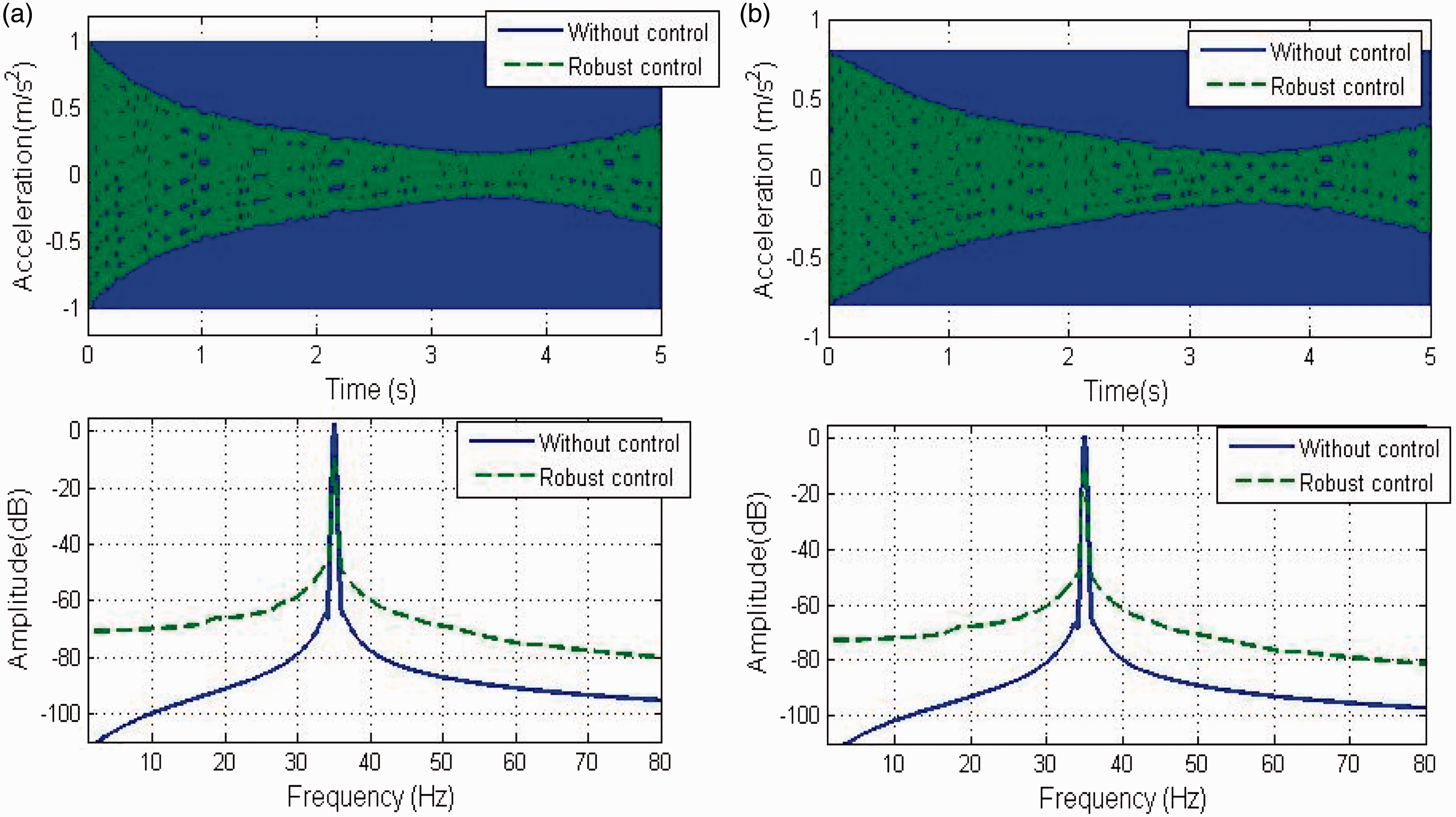

H_∞ control experiments for a MIMO control system

The diagram of MIMO feedback control system is shown in Figure 12, the system is a two-input two-output feedback control system. The voltage signal proportional to the acceleration signal from the low-pass filter can be regarded as error signals, as shown in E1 and E4 of Figure 11. E1 represents the voltage signal from the conditioning and filtered 1# acceleration signal, and E4 represents the voltage signal from the conditioning and filtered 4# acceleration signal. The filter output port connects with the A/D port of the dSPACE1103 system's wiring panel CLP1103. The control board DS1103 is a kind of controller hardware, depending on the designed controller to calculate the control amount. The calculation for controller adopts fixed-step calculation method, of which the step is 0.0001 and the solver is ode8. After crossing D/A converter, the control amount outputs two control signals, namely U1 and U4 as shown in Figure 11. The amplitudes of the two control signals are confined to ±5 V. The control signal U1 goes across 1# power amplifier, and then drives l# electromagnetic actuator to output control force; after going across 4# power amplifier, the control signal U4 drives 4# electromagnetic actuator to output control force. On the coordinative role of the two actuators, the vibration from frequency fluctuation disturbance generated by the motor above the 1#actuator can be inhibited.

Figure 12.

Schematic diagram of the MIMO feedback control system. MIMO: multiple input multiple output.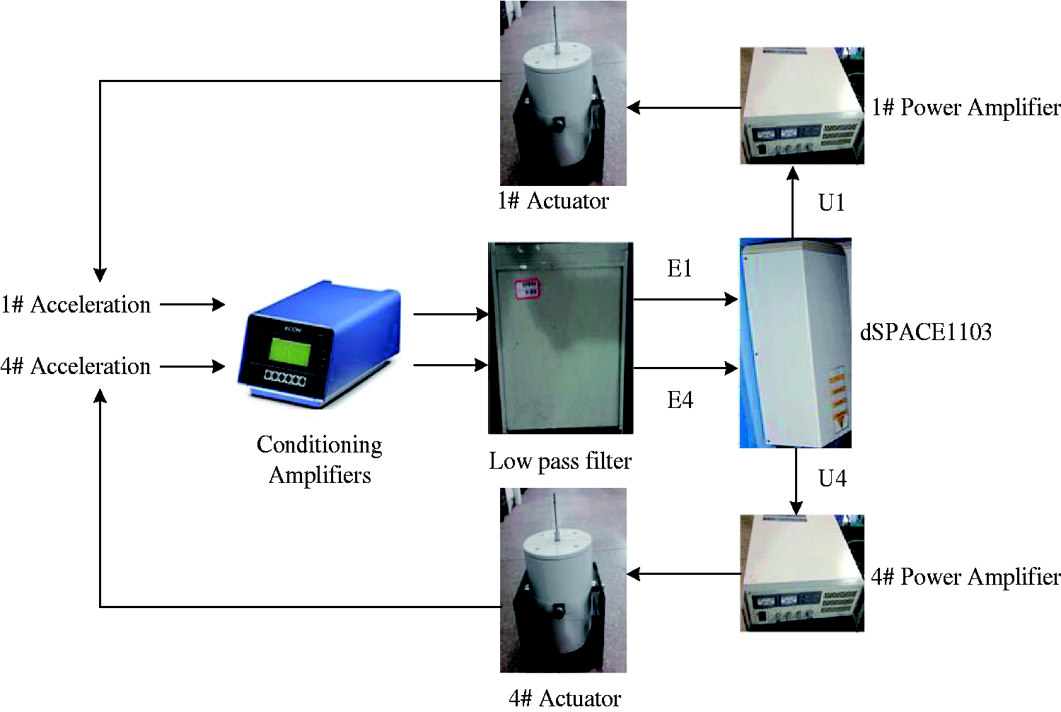

In the experiments, two different controllers are designed to suppress the disturbances with dominant frequency of 30 and 35 Hz. When the frequency is 30 Hz, we choose the speed of the motor above 1# actuator 1800 r/min, when the frequency is 35 Hz, we choose the speed of the motor above 1# actuator 2100 r/min.

When the speed of the motor above 1# actuator is 1800 r/min, the active vibration control experiment is conducted according to Figure 11, and experimental results are shown in Figures 13 and 14, respectively. Without control, the two control signals are 0, and the amplitudes of the error signals are approximately 0.5 and 0.3 m/s². After the robust control, two control signals gradually increase and eventually approach a steady state; the two error signals achieve fast convergence, and their amplitudes are greatly reduced. In the interception map, the signals are used as error signals without control from 0 to 5 s and the signals are used as error signals with robust control from 5 to 11 s. The RMS values of error signal E1 before and after the control are, respectively, 0.3689 and 0.0823, so the RMS value is decreased 77.68%. The RMS values of error signal E4 before and after the controls are, respectively, 0.2597 and 0.0659, which indicates a 74.64% decrease in the RMS value.

Figure 13.

Time-domain diagram of error signals and control signals when the speed of motor is 1800 r/min.

Figure 14.

Self-power spectrum of the error signals of 30 Hz.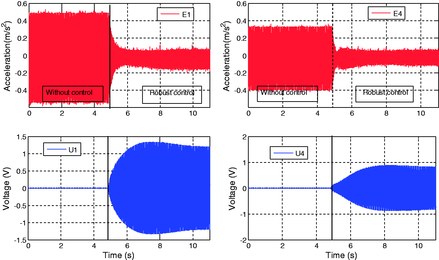

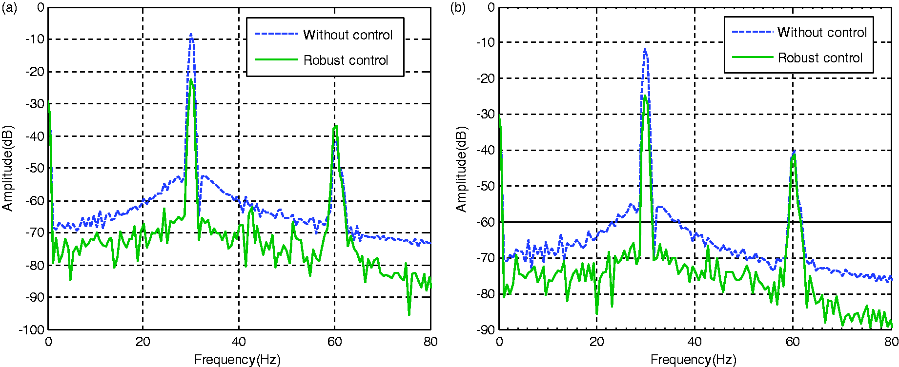
Figure 14(a) and (b), respectively, represent the self-power spectrum of the error signals E1 and E4 before and after the control, where the amplitudes of the frequency components in the range of about 30 Hz within the error signals E1 and E4 are greatly reduced by 13.91 and 13.16 dB, respectively, while other frequency components show no significant changes.

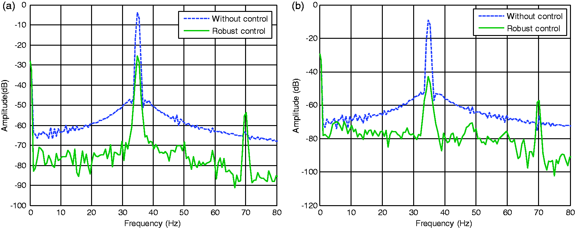
When the speed of the motor above 1# actuator is 2100 r/min, experimental results are shown in Figures 15 and 16, respectively. After the robust control, two control signals gradually increase and eventually approach a steady state; the two error signals achieve fast convergence, and their amplitudes are greatly reduced. In the interception map, the signals are used as error signals without control from 0 to 4 s and the signals are used as error signals with robust control from 4 to 10 s. The RMS values of error signal E1 before and after the control are, respectively, 0.6258 and 0.0614, so the RMS value is decreased 90.19%. The RMS values of error signal E4 before and after the control are, respectively, were 0.3369 and 0.0335, which indicates a 90.06% decrease in the RMS value. Figure 16(a) and (b), respectively, represents the self-power spectrum of the error signals E1 and E4 before and after the control, where the amplitudes of the frequency components in the range of about 30 Hz within the error signals E1 and E4 are greatly reduced by 22.48 and 33.88 dB respectively, while other frequency components show no significant changes.

Figure 15.

Time-domain diagram of error signals and control signals when the speed of motor is 2100 r/min.

Figure 16.

Self-power spectrum of the error signals of 35 Hz.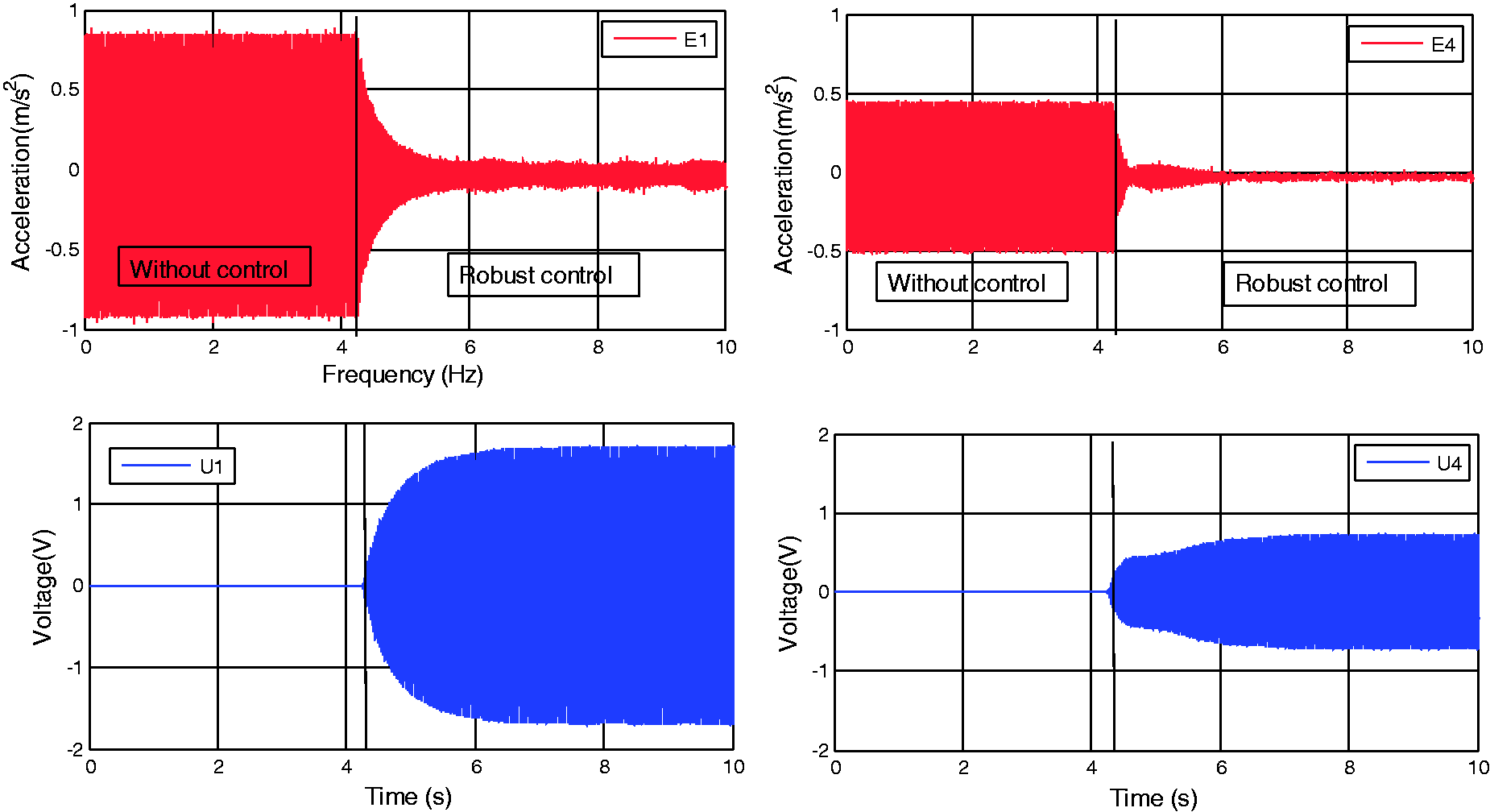

Conclusion

The system identification method is adopted to establish two-input and two-output continuous transfer function model of the control channel for the floating raft vibration isolation system, and the model can accurately describe the dynamic characteristics of the controlled object. The H_∞ controller is designed with the shaping design method based on mixed sensitivity problem and the selection method of weighting function is described. The H_∞ controller is designed for a MIMO system to suppress single frequency-varying disturbance. Simulation analysis is conducted against the designed controller, and the results show that the amplitudes of the dominant frequencies are attenuated more than 10 dB before and after the robust control. An actual floating raft vibration isolation system is built for the single excitation source multichannel control experiments. Each experiment achieves good vibration isolation effect, the RMS values of error signals drop by more than 74% before and after the control, and the amplitudes of the dominant frequency have fallen more than 13 dB. Experimental results show that the controller can effectively suppress frequency-varying disturbance.