Dynamic characteristics analysis of a high-speed-level gear transmission system of a wind turbine considering a time-varying wind load and an electromagnetic torque disturbance

Abstract

A high-speed-level gear transmission system model of a wind turbine is presented considering a time-varying wind load and an electromagnetic torque disturbance, along with eccentricity, dynamic backlash, and friction force. The auto-regressive model is employed for simulating the time-varying wind load in the realistic wind field as external excitation. A doubly fed induction generator model of the wind turbine is established to calculate the disturbance quantity of electromagnetic torque. The nonlinear differential equations of the system are strictly deduced using Lagrange equation and solved by the fourth-order Runge-Kutta method. The effect of friction on the dynamic response of the high-speed-level gear transmission system is analyzed with the time-varying wind load and the electromagnetic torque disturbance. These results show that the friction force is critical because frequency amplitude and components can be changed by it. The friction force also enlarges vibration displacement. The low-frequency components in the vertical direction are affected gravely by the friction force without electrical disturbance. In addition, sidebands exist in the vicinity of the low-frequency parts as the electromagnetic torque disturbance appears at the output end. The amplitude of the low-frequency component is further increased because of electromagnetic torque disturbance. This shows the frequency characteristics of the slight gear system fault. The study offers some fresh references into the design and diagnosis of the gear system.

Introduction

In recent years, research on nonlinear dynamic methods has been improved continuously. Many mathematical methods open a new door for the establishment of nonlinear dynamic analysis of a gear system.^1–5 To ensure the stability and reliability of gear transmission systems, the dynamic characteristics of the gearbox should be investigated. Many outstanding scholars have researched a gear transmission system for different purposes and many outstanding results were obtained.^6–14 Their study subjects included the planetary gear torsion vibration model, bending-torsional coupled model, and unipolar spur gear-rotor-bearing couple model.

In order to analyze approximately realistic vibration on the gear system of the wind turbine, scholars in mounting numbers started to apply different models to simulate the realistic wind speed. The wind load research is increasingly complex. Chen et al. ¹⁵ established a random wind speed as external excitation and the vibration response and dynamic mesh force mean are analyzed. Qin et al. ¹⁶ employed the auto-regressive (AR) model to simulate time-varying wind speed and load. A planetary gear model of the wind turbine was built using the lumped-mass method. It is depicted for the vibration of the planetary gear transmission system and dynamic mesh process in detail. Qin et al. ¹⁷ used Weibull distribution to simulate time-varying wind speed and load. The vibration displacement, velocity, and dynamic mesh force of the planetary gear transmission system were analyzed. Zhou et al. ¹⁸ used sparse least squares support vector machine (SL-SVM) to simulate the wind speed of the exact wind field and wind load. The coupled planetary gear-bearing model was established to research vibration displacement of all the parts and dynamic mesh force. Li et al. ¹⁹ researched the effect of non-torque loads on wind turbine drivetrain. Chuang et al. ²⁰ studied the influence of second-order wave excitation loads on the coupled response of an offshore floating wind turbine.

In addition, the backlash is a critical factor to ensure stable and reliable running. Chen et al. ²¹ investigated dynamic backlash with the fractal feature and effect of the dynamic backlash on the 2-DOF gear system. Lu et al. ²² researched bifurcation characteristics on the gear transmission system with the stochastic backlash, which made an influence in the system responses. Liu et al. ²³ investigated the dynamic backlash, which was affected by the dynamic center distance. The effect of the dynamic backlash and dynamic mesh angle was studied. Liu et al. ²⁴ investigated the effect of the compound dynamic backlash on the gear-rotor-bearing transmission system. The response and frequency features of gear root crack faults were analyzed.

Although many types of research have been dedicated to investigating the gear system dynamic model of wind turbine generators considering shafts, bearings, or flexible systems, it is worth noting that the previous analysis for different excitation effect on the gear system of wind turbine generator was separately studied. Dynamic behaviors with dynamic backlash, time-varying wind load (front input excitation of gear system), electromagnetic torque disturbance (end output excitation of gear system) and friction force simultaneously are rarely researched. In addition, it is noteworthy that earlier researches of time-varying input/output load were mainly focused on the variation of force and displacement and the frequency analysis was ignored. Therefore, this paper is devoted to the theoretical study of the dynamic characteristics of the high-speed-level gear transmission system of the wind turbine under the simultaneous action of multiple excitations. A high-speed-level gear transmission system dynamic model of wind turbine generator is established using the lumped-mass method considering a time-varying wind load and an electromagnetic torque disturbance, along with eccentricity, dynamic backlash, and friction force. The nonlinear differential equations are deduced using the Lagrange equation. AR model is employed for simulating the realistic wind field and deducing varying wind load. In the case of variable wind load, a small grid voltage drop fault is imposed on the output, and electromagnetic torque variation is calculated by the doubly fed induction generator (DFIG) model. The equations are solved by the Runge-Kutta method. The vibration response of the gear system is attained. This displacement and frequency feature of parts are depicted in detail, which can provide a fundamental reference for the optimal design and monitor the gear system of the wind turbine.

Auto-regressive wind speed model

Pulsating wind speed can be considered the arbitrariness of the wind sites, wind spectrum characteristics, building characteristics and other conditions, which is simulated using a linear filtering method based on the autoregressive model. The pulsating wind speed is more representative than the actual observation record on the wind sites. The simulated method is widely used for simulating pulsating wind speed. In this model, a random series of white noise with zero mean is passed through a linear filter and its output is a stationary random process with specified spectral characteristics.

According to wind speed observational data, instantaneous wind speed consists of two elements including the average wind with a period of more than 10 min and the pulsating wind with a period of a few seconds.

The AR model of time-history V(t) column vector of spatially correlated pulsating wind speed with M points can be expressed as

$$V(t)=-{\displaystyle \sum _{k=1}^p{\psi }_k}V(t-k\Delta t)+Ln(t)$$

(1)

where p is the order of AR model, $\Delta t$ is the step value of simulated wind speed time-histories, ${\psi }_k$ is autoregressive coefficient matrix of the AR model. $n_i(t)$ is a mutual independent normal random process, the mean value is zero and the variance is one. L is M order lower triangular matrix.

The time history of wind speed can be further obtained. It can be described as

$$V_{th}=\overline{V}+V(t)$$

(2)

where $\overline{V}$ is mean wind speed, and $V(t)$ is the variation value of pulsating wind.

A high-speed-level gear transmission system dynamic model of a wind turbine

The research object in this paper is a high-speed-level gear transmission system of a wind turbine. Its structure is shown in Figure 1, marked red.

Figure 1.

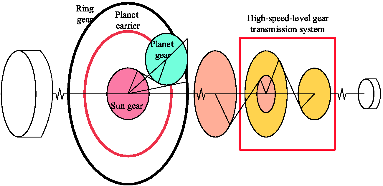
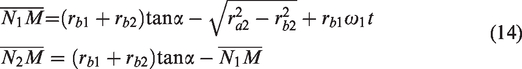
The planetary gear transmission of wind turbine structure sketch.

The lumped mass model of the high-speed-level gear transmission system

In this section, considering the lumped mass model is adopted to conduct the dynamic modeling of the high-speed-level gear transmission system aiming to preliminarily study the dynamic characteristics of the wind turbine gear system. This section is simplified as follows:

Ignoring assembly errors, the gear shaft is strictly central to the input and output ends.

The bearing is equivalent to a spring bearing with fixed stiffness.

The bearing damping and meshing damping are equivalent to viscous damping

The thermal deformation in the gearbox is ignored.

Ignoring the torque loss and the torque control feedback of the wind turbine, the external excitation is calculated strictly according to the transmission ratio.

The gear mesh parameters are simulated by springs and dampers. The 16-DOF coupled bending-torsional spur gear transmission system model is shown in Figure 2.

Figure 2.

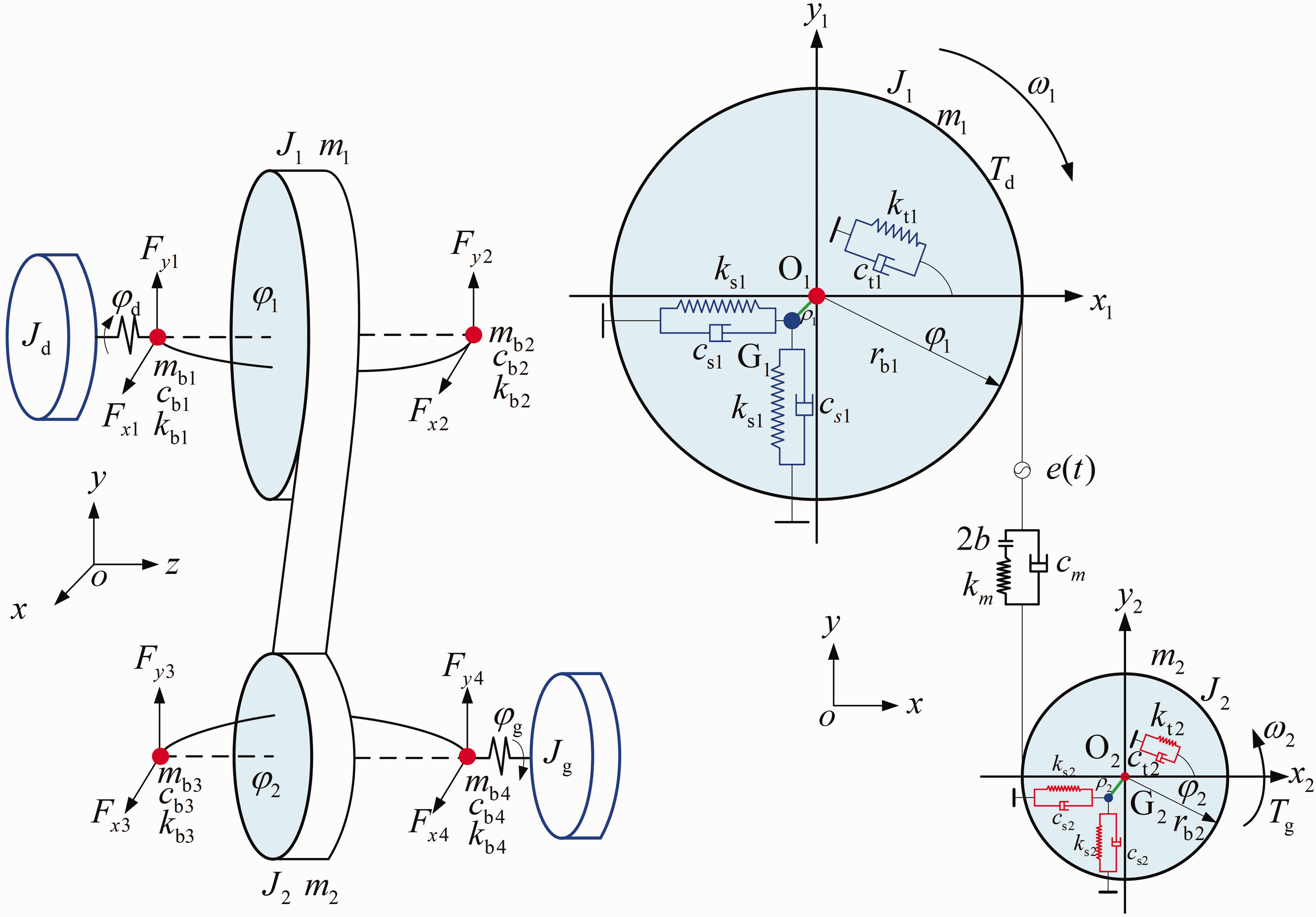
The 16-DOF bending-torsional coupled spur gear transmission system.

According to the established dynamic model, φ _i (i = 1, 2, d, g) are respectively angle displacements of gear, pinion, input and output. The angle displacements are composed of an angle displacement ω_it(i = 1,2) and microscopic displacement θ_i(t). The equations are defined to

$$\begin{array}{c}{\phi }_1={\omega }_{1}t+{\theta }_1,{\phi }_2={\omega }_{2}t+{\theta }_2\\ {\phi }_d={\omega }_{1}t+{\theta }_d,{\phi }_g={\omega }_{2}t+{\theta }_g\end{array}$$

(3)

Because the gear center and the center of gravity are different, the relationship of them is given by

$$\begin{array}{c}{x}_{g1}=x_1+{\rho }_1\cos {\phi }_1,y_{g1}=y_1+{\rho }_1\text{sin}{\phi }_1\\ x_{g2}=x_2+{\rho }_2\cos {\phi }_2,y_{g2}=y_2+{\rho }_1\sin {\phi }_2\end{array}$$

(4)

where ${\rho }_i(i=1,2)$ is eccentricity, gears’ center and center of gravity are O₁(x₁, y₁), O₂(x₂, y₂) and G₁(x_g1, y_g1), G₂(x_g2, y_g2).

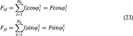
The elastic deformation of the shafts can be determined as

$$\begin{array}{c}{\delta }_{x1}=x_1-{\xi }_1{x}_{b2}-{\xi }_2{x}_{b1},\hspace{1em}{\delta }_{y1}=x_1-{\xi }_1{y}_{b2}-{\xi }_2{y}_{b1}\\ {\delta }_{x2}=x_2-{\xi }_3{x}_{b4}-{\xi }_4{x}_{b3},\hspace{1em}{\delta }_{y2}=y_2-{\xi }_3{y}_{b4}-{\xi }_4{y}_{b3}\end{array}$$

(5)

where ξ _i =l_bi/l_j (i= 1, 2, 3, 4; j=1, 2), l_bi represent the distances between gear’s center and center of bearing, and l_j are the length of shafts.

The deformation transmission error (DTE) caused by gear meshing along the line of action is described as

$$\begin{array}{l}\delta \left(t\right)=(r_{b1}{\phi }_1-r_{b2}{\phi }_2)+(y_{g1}-y_{g2})-e\left(t\right)\\ \hspace{1em}\hspace{1em}=(r_{b1}{\theta }_1-r_{b2}{\theta }_2)+(y_1-y_2+{\rho }_1\sin {\phi }_1-{\rho }_2\sin {\phi }_2)-e\left(t\right)\end{array}$$

(6)

where $e(t)$ is static transmission error e(t)=e₀+e_rsin(ω_mt + φ_m), e₀ and e_r represent mean and amplitude of the error, ω_m is mesh frequency ω_m=2πn₁z₁/60(2πn₂z₂/60). z₁ and z₂ are the numbers of teeth, and n₁ and n₂ are the rotating velocities of gears.

The dynamic force is defined as

$$F_m\text{=}{k}_{m}f(\delta (t))+c_m\dot{\delta }(t)$$

(7)

where $k_m$ is the gear mesh stiffness, $c_m$ is the mesh damping, and $f(\delta (t))$ is the nonlinear function. It is given by

$$f(\delta (t))=\{\begin{array}{ll}\delta (t)-(1-\varpi )b_h(t)& \delta (t)>b_h(t)\\ \varpi b_h(t)& -b_h(t)<\delta (t)<b_h(t),0\le \varpi \le 1\\ \delta (t)+(1-\varpi )b_h(t)& \delta (t)<-b_h(t)\end{array}$$

(8)

where $\varpi$ represents the backlash nonlinear coefficient and b_h(t) represents dynamic backlash.

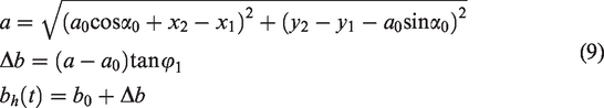
The dynamic backlash b_h(t) consists of a fixed backlash and a backlash variation value. The fixed backlash $b_0$ is generated by the manufacture and fabrication of gears. When the gear system vibrates, the gear center distance a must be changed and the backlash variation value $\Delta b$ is generated. Based on the geometrical relationship, the dynamic backlash b_h(t) is defined by

$$\begin{array}{l}a=\sqrt{{(a_0\cos {\alpha }_0+x_2-x_1)}^2+{(y_2-y_1-a_0\sin {\alpha }_0)}^2}\\ \Delta b=(a-a_0)\tan {\phi }_1\\ b_h(t)=b_0+\Delta b\end{array}$$

(9)

where $a_0$ represents theoretical center distance.

The Friction force of the gear system model is shown in Figure 3. The speeds $V_{m1}$ and $V_{m2}$ on the mesh point M of gear can be described as

$$V_{m1}={\omega }_1\overline{O_{1}M},V_{m2}={\omega }_2\overline{O_{2}M}$$

(10)

Figure 3.

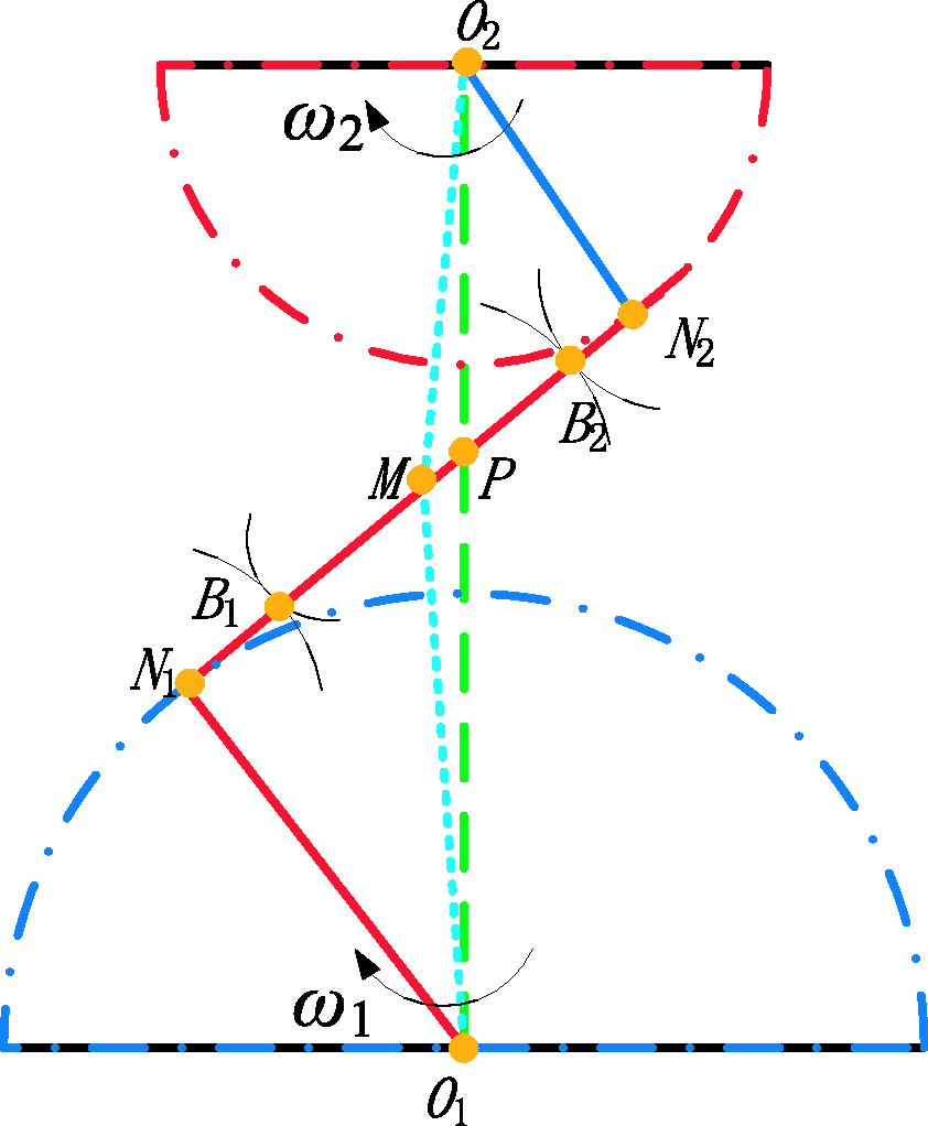
Simplified sketch of meshing.

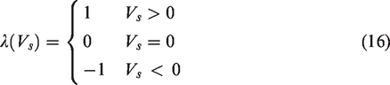
The sliding speed V_s on the mesh point M is given by

$$V_s=V_{m1}\sin {\phi }_1-V_{m2}\sin {\phi }_2$$

(11)

According to the geometrical relationship, the friction arm $\overline{N_{1}M},\overline{N_{2}M}$ can be described as

$$\overline{N_{1}M}=\overline{O_{1}M}\sin {\phi }_1,\overline{N_{2}M}=\overline{O_{2}M}\sin {\phi }_2$$

(12)

The sliding speed also can be changed as

$$V_s={\omega }_1\overline{N_{1}M}+{\omega }_2\overline{N_{2}M}$$

(13)

The friction arms $\overline{N_{1}M},\overline{N_{2}M}$ can be defined by

$$\begin{array}{l}\overline{N_{1}M}\text{=}(r_{b1}+r_{b2})\tan \alpha -\sqrt{r_{a2}^2-r_{b2}^2}+r_{b1}{\omega }_{1}t\\ \overline{N_{2}M}=(r_{b1}+r_{b2})\tan \alpha -\overline{N_{1}M}\end{array}$$

(14)

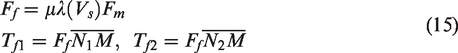
The friction force and torques are given by

$$\begin{array}{l}{F}_f=\mu \lambda (V_s)F_m\\ T_{f1}=F_f\overline{N_{1}M},T_{f2}=F_f\overline{N_{2}M}\end{array}$$

(15)

where $\mu$ is the friction coefficient and $\lambda (V_s)$ is the direction coefficient.

$$\lambda (V_s)=\{\begin{array}{ll}1& V_s>0\\ 0& V_s=0\\ -1& V_s<0\end{array}$$

(16)

Dynamic model of ball bearing

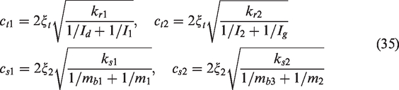
The ball-bearing model is shown in Figure 4. Based on the ball model, the v_i and v_o represent the contact point velocities between the rolling elements and inner/outer rings are given by

$$v_i={\omega }_i\cdot r,v_o={\omega }_o\cdot R$$

(17)

where R and r are radii of the inner and outer ring. ω_i and ω_o are the angular velocities of inner and outer rings. The velocity of the cage is given by

$$v_b=(v_i+v_o)/2=({\omega }_{o}R+{\omega }_{i}r)/2$$

(18)

Figure 4.

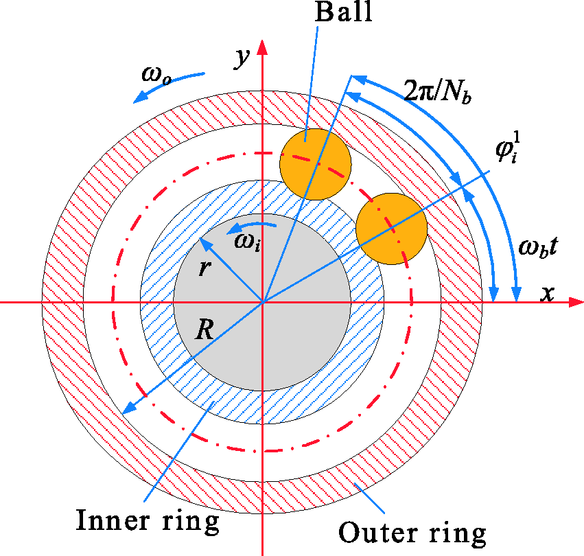
Rolling bearing model.

The angular velocity of the cage can be defined by

$${\omega }_b=2v_b/(R+r)={\omega }_i·r/(R+r)$$

(19)

The angular displacement ${\phi }_i^1$ of the ith rolling element can be described as

$${\phi }_i^1={\omega }_b\cdot t+2\pi \left(i-1\right)/N_b,\left(i=1,2,3,\cdots N_b\right)$$

(20)

where N_b is the number of the rolling ball.

The deformation of the ith rolling ball can be given by

$${\delta }_i^1=x\cos {\phi }_i^1+y\sin {\phi }_i^1-{\gamma }_0$$

(21)

where γ₀ represents bearing clearance. The Hertz contact theory is employed for computing contact force. The contact force of the ith rolling element f_i can be determined as

$$f_i=K_b{\left(x\cos {\phi }_i^1+y\sin {\phi }_i^1-{\gamma }_0\right)}^{3/2}\cdot H\left(x\cos {\phi }_i^1+y\sin {\phi }_i^1-{\gamma }_0\right)$$

(22)

Therefore, the bearing force can be defined by

$$\begin{array}{l}{F}_{xj}={\displaystyle \sum _{i=1}^{N_b}{f}_i}\cos {\phi }_i^1=F\cos {\phi }_i^1\\ F_{yj}={\displaystyle \sum _{i=1}^{N_b}{f}_i}\sin {\phi }_i^1=F\sin {\phi }_i^1\end{array}$$

(23)

External excitation of the system

The variation load of the wind turbine input terminal caused by the AR pulsating wind speed is set to system external excitation. Based on the aerodynamics, the Output power of wind turbine impeller $P_o$ is defined to

$$P_o=\frac{1}{2}{\rho }_a\pi r_w^2{V}_{th}^3{C}_p$$

(24)

where ${\rho }_a$ is the air density, $r_w$ is the rotor radius, $C_p$ is the rotor power coefficient.

The wind wheel input torque $T_{\text{in}}$ is given by

$$T_{\text{in}}=P_o/{\omega }_w$$

(25)

where ${\omega }_w$ is the angular velocity of the wind wheel.

Without calculating the energy loss, the torque of each transmission system can be converted through the transmission ratio.

After considering electrical disturbance, the DFIG system model, as shown in Figure 5, is needed to establish.

Figure 5.

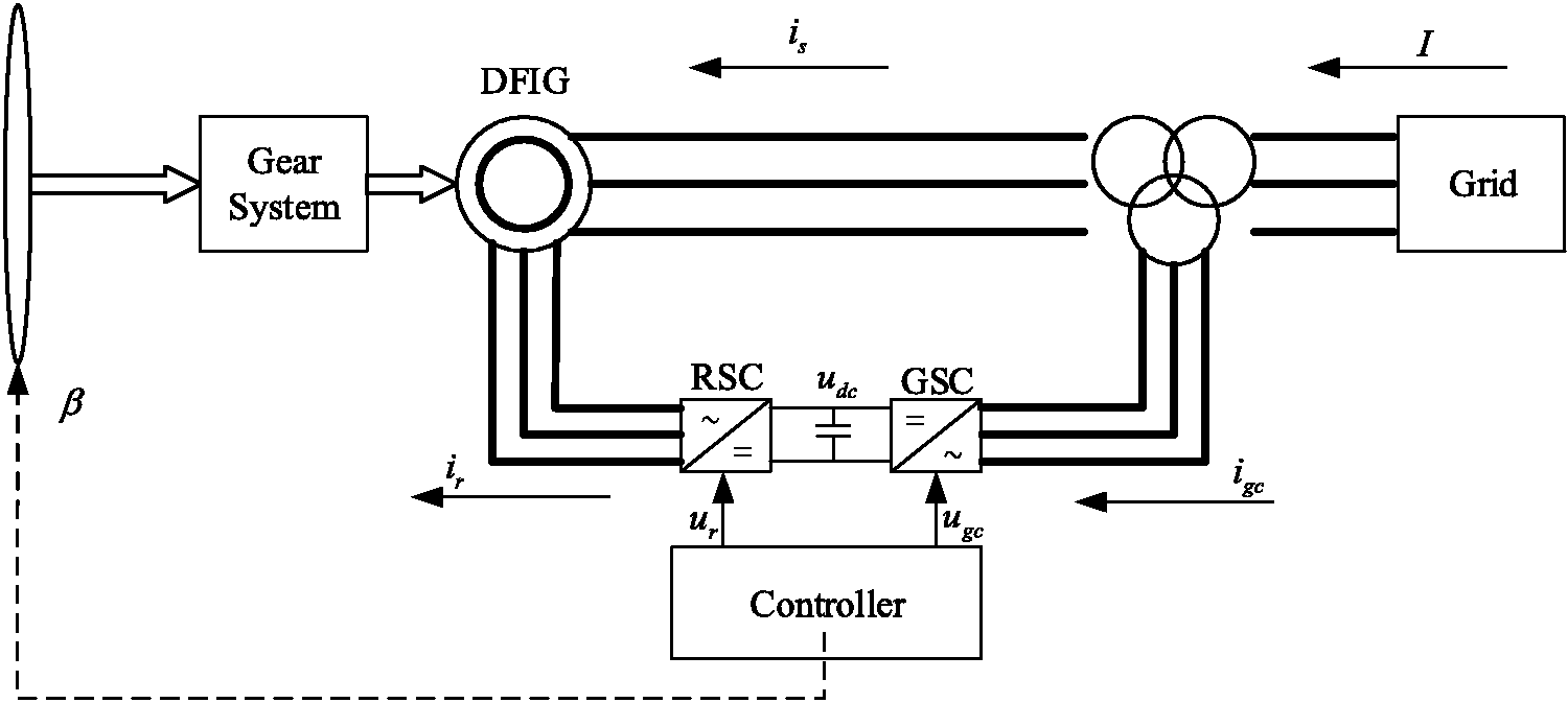
DFIG model of wind turbine.

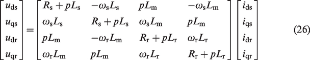
In the synchronous rotation coordinates, the voltage equation of the double-feedback wind generator is expressed as

$$\left[\begin{array}{l}{u}_{\text{ds}}\\ u_{\text{qs}}\\ u_{\text{dr}}\\ u_{\text{qr}}\end{array}\right]\text{=}\left[\begin{array}{llll}{R}_{\text{s}}+p{L}_{\text{s}}& -{\omega }_{\text{s}}{L}_{\text{s}}& p{L}_{\text{m}}& -{\omega }_{\text{s}}{L}_{\text{m}}\\ {\omega }_{\text{s}}{L}_{\text{s}}& R_{\text{s}}+p{L}_{\text{s}}& {\omega }_{\text{s}}{L}_{\text{m}}& p{L}_{\text{m}}\\ p{L}_{\text{m}}& -{\omega }_{\text{r}}{L}_{\text{m}}& R_{\text{r}}+p{L}_{\text{r}}& {\omega }_{\text{r}}{L}_{\text{r}}\\ {\omega }_{\text{r}}{L}_{\text{m}}& p{L}_{\text{m}}& {\omega }_{\text{r}}{L}_{\text{r}}& R_{\text{r}}+p{L}_{\text{r}}\end{array}\right]\left[\begin{array}{l}{i}_{\text{ds}}\\ i_{\text{qs}}\\ i_{\text{dr}}\\ i_{\text{qr}}\end{array}\right]$$

(26)

where $u_{\text{ds}}$ , $u_{\text{qs}}$ , $u_{\text{dr}}$ , $u_{\text{qr}}$ is the voltage under the d-q axis of the generator stator and rotor; $i_{\text{ds}}$ , $i_{\text{qs}}$ , $i_{\text{dr}}$ , are $i_{\text{qr}}$ is current under the d-q axis of the generator stator and rotor; ${\omega }_{\text{s}}$ is the synchronous angular velocity; ${\omega }_{\text{r}}$ is the angular velocity of the rotor; $R_{\text{s}}$ , $R_{\text{r}}$ is the equivalent resistance of stator and rotor. The stator equivalent inductance and the rotor equivalent mutual inductance are $L_{\text{s}}$ , $L_{\text{r}}$ . $L_{\text{m}}$ is the equivalent mutual inductance between stator and rotor, and p is the differential operator.

The electromagnetic torque of the double-feedback wind turbine is expressed as

$$T_{\text{e}}=1.5n_{\text{p}}{L}_{\text{m}}(i_{\text{qs}}{i}_{\text{dr}}-i_{\text{ds}}{i}_{\text{qr}})$$

(27)

where $T_{\text{e}}$ is the electromagnetic torque, and $n_{\text{p}}$ is the polar logarithm of the wind generator.

Mathematical model of the system

The mathematical vibration model of the high-speed-level gear transmission system can be derived by Lagrange’s equation. It is clearly expressed that the kinetic energy T, the dissipation energy R and the potential energy U, as shown in equations (28) to (32), can be calculated by the kinetic knowledge in the generalized coordinates of the high-speed-level gear transmission system.

It is easily understood that the gear system includes 16-DOF in this coordinate, and its expressing can be given by

$$\mathbf{X}=\left[\begin{array}{llllllllllllllll}{\theta }_d& x_1& y_1& {\theta }_1& x_2& y_2& {\theta }_2& x_{b1}& y_{b1}& x_{b2}& y_{b2}& x_{b3}& y_{b3}& x_{b4}& y_{b4}& {\theta }_g\end{array}\right]$$

(28)

The kinetic energy T can be calculated as follows

$$T=\frac{1}{2}[m_i\left({\dot{x}}_{g1}^2+{\dot{y}}_{g1}^2\right)+m_{bi}\left({\dot{x}}_{b1}^2+{\dot{y}}_{b1}^2\right)+J_d{\dot{\phi }}_d^2+J_1{\dot{\phi }}_1^2+J_2{\dot{\phi }}_2^2+J_g{\dot{\phi }}_g^2]$$

(29)

The dissipation energy R can be expressed in consideration of damping in the system as follows

$$R=\frac{1}{2}{c}_{si}({\dot{\delta }}_{xi}^2+{\dot{\delta }}_{yi}^2)+\frac{1}{2}{c}_{t1}{({\dot{\phi }}_1-{\dot{\phi }}_d)}^2+\frac{1}{2}{c}_{t2}{({\dot{\phi }}_g-{\dot{\phi }}_2)}^2$$

(30)

Taking into account the gears, shaft and bearings deformations, the potential energy U can be given by

$$U=\frac{1}{2}{k}_{si}\left({\delta }_{xi}^2+{\delta }_{yi}^2\right)+\frac{1}{2}{k}_{t1}{\left({\phi }_1-{\phi }_d\right)}^2+\frac{1}{2}{k}_{t2}{\left({\phi }_g-{\phi }_2\right)}^2$$

(31)

Considering gears’ gravity and input/output torque, the force vector F of the system in the generalized coordinate can be defined by

$$\mathbf{F}=\left[\begin{array}{llllllllllllllll}{T}_d& 0& -m_{\text{1}}g& 0& 0& -m_{2}g& 0& 0& 0& 0& 0& 0& 0& 0& 0& T_g\end{array}\right]$$

(32)

Lagrange’s equation is expressed by

$$\frac{\partial }{\partial t}\left(\frac{\partial T}{\partial \dot{\mathbf{X}}}\right)-\frac{\partial T}{\partial \mathbf{X}}+\frac{\partial U}{\partial \mathbf{X}}+\frac{\partial R}{\partial \dot{\mathbf{X}}}\mathbf{=F}$$

(33)

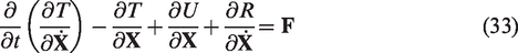
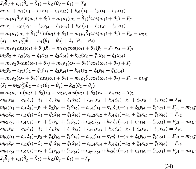
When equations (28) to (32) are substituted into Lagrange’s equation, as shown in equation (33), the vibration differential equations can be written as follows

$$\begin{array}{l}{J}_d{\ddot{\theta }}_d+c_{t1}\left({\dot{\theta }}_d-{\dot{\theta }}_1\right)+k_{t1}\left({\theta }_d-{\theta }_1\right)=T_d\\ m_1{\ddot{x}}_1+c_{s1}\left({\dot{x}}_1-{\xi }_2{\dot{x}}_{b1}-{\xi }_1{\dot{x}}_{b2}\right)+k_{s1}\left(x_1-{\xi }_2{x}_{b1}-{\xi }_1{x}_{b2}\right)\\ =m_1{\rho }_1{\ddot{\theta }}_1\sin \left({\omega }_{1}t+{\theta }_1\right)+m_1{\rho }_1{\left({\omega }_1+{\dot{\theta }}_1\right)}^2\cos \left({\omega }_{1}t+{\theta }_1\right)-F_f\\ m_1{\ddot{y}}_1+c_{s1}\left({\dot{y}}_1{\hspace{0.17em}}_1-{\xi }_2{\dot{y}}_{b1}-{\xi }_1{\dot{y}}_{b2}\right)+k_{s1}\left(y_1-{\xi }_2{y}_{b1}-{\xi }_1{y}_{b2}\right)\\ =m_1{\rho }_1{\left({\omega }_1+{\dot{\theta }}_1\right)}^2\sin \left({\omega }_{1}t+{\theta }_1\right)-m_1{\rho }_1{\ddot{\theta }}_1\cos \left({\omega }_{1}t+{\theta }_1\right)-F_m-m_{1}g\\ \left(J_1+m_1{\rho }_1^2\right){\ddot{\theta }}_1+c_{t1}\left({\dot{\theta }}_1-{\dot{\theta }}_d\right)+k_{t1}\left({\theta }_1-{\theta }_d\right)\\ =m_1{\rho }_1\sin \left({\omega }_{1}t+{\theta }_1\right){\ddot{x}}_1-m_1{\rho }_1\cos \left({\omega }_{1}t+{\theta }_1\right){\ddot{y}}_1-F_m{r}_{b1}+T_{f1}\\ m_2{\ddot{x}}_2+c_{s2}\left({\dot{x}}_2-{\xi }_4{\dot{x}}_{b3}-{\xi }_3{\dot{x}}_{b4}\right)+k_{s2}\left(x_2-{\xi }_4{x}_{b3}-{\xi }_3{x}_{b4}\right)\\ =m_2{\rho }_2{\ddot{\theta }}_2\sin \left({\omega }_{2}t+{\theta }_2\right)+m_2{\rho }_2{\left({\omega }_2+{\dot{\theta }}_2\right)}^2\cos \left({\omega }_{2}t+{\theta }_2\right)+F_f\\ m_2{\ddot{y}}_2+c_{S2}\left({\dot{y}}_2-{\xi }_4{\dot{y}}_{b3}-{\xi }_3{\dot{y}}_{b4}\right)+k_{s1}\left(y_2-{\xi }_4{y}_{b3}-{\xi }_3{y}_{b4}\right)\\ =m_2{\rho }_2{\left({\omega }_2+{\dot{\theta }}_2\right)}^2\sin \left({\omega }_{2}t+{\theta }_2\right)-m_2{\rho }_2{\ddot{\theta }}_2\cos \left({\omega }_{2}t+{\theta }_2\right)-F_m-m_{2}g\\ \left(J_2+m_2{\rho }_2^2\right){\ddot{\theta }}_2+c_{t2}\left({\dot{\theta }}_2-{\dot{\theta }}_g\right)+k_{t2}\left({\theta }_2-{\theta }_g\right)\\ =m_2{\rho }_2\sin \left({\omega }_{2}t+{\theta }_2\right){\ddot{x}}_2-m_2{\rho }_2\cos \left({\omega }_{2}t+{\theta }_2\right){\ddot{y}}_2-F_m{r}_{b2}-T_{f2}\\ m_{b1}{\ddot{x}}_{b1}+c_{s1}{\xi }_2\left(-{\dot{x}}_1+{\xi }_2{\dot{x}}_{b1}+{\xi }_1{\dot{x}}_{b2}\right)+c_{bx1}{\dot{x}}_{b1}+k_{s1}{\xi }_2\left(-x_1+{\xi }_2{x}_{b1}+{\xi }_1{x}_{b2}\right)=F_{x1}\\ m_{b1}{\ddot{y}}_{b1}+c_{s1}{\xi }_2\left(-{\dot{y}}_1+{\xi }_2{\dot{y}}_{b1}+{\xi }_1{\dot{y}}_{b2}\right)+c_{by1}{\dot{y}}_{b1}+k_{s1}{\xi }_2\left(-y_1+{\xi }_2{y}_{b1}+{\xi }_1{y}_{b2}\right)=F_{y1}-m_{b1}g\\ m_{b2}{\ddot{x}}_{b2}+c_{s1}{\xi }_1\left(-{\dot{x}}_1+{\xi }_2{\dot{x}}_{b1}+{\xi }_1{\dot{x}}_{b2}\right)+c_{bx2}{\dot{x}}_{b2}+k_{s1}{\xi }_1\left(-x_1+{\xi }_2{x}_{b1}+{\xi }_1{x}_{b2}\right)=F_{x2}\\ m_{b2}{\ddot{y}}_{b2}+c_{s1}{\xi }_1\left(-{\dot{y}}_1+{\xi }_2{\dot{y}}_{b1}+{\xi }_1{\dot{y}}_{b2}\right)+c_{by2}{\dot{y}}_{b1}+k_{s1}{\xi }_1\left(-y_1+{\xi }_2{y}_{b1}+{\xi }_1{y}_{b2}\right)=F_{y2}-m_{b2}g\\ m_{b3}{\ddot{x}}_{b3}+c_{s2}{\xi }_4\left(-{\dot{x}}_2+{\xi }_4{\dot{x}}_{b3}+{\xi }_3{\dot{x}}_{b4}\right)+c_{bx3}{\dot{x}}_{b3}+k_{s2}{\xi }_4\left(-x_2+{\xi }_4{x}_{b3}+{\xi }_3{x}_{b4}\right)=F_{x3}\\ m_{b3}{\ddot{y}}_{b3}+c_{s2}{\xi }_4\left(-{\dot{y}}_2+{\xi }_4{\dot{y}}_{b3}+{\xi }_3{\dot{y}}_{b4}\right)+c_{by3}{\dot{y}}_{b3}+k_{s2}{\xi }_4\left(-y_2+{\xi }_4{y}_{b3}+{\xi }_3{y}_{b4}\right)=F_{y3}-m_{b3}g\\ m_{b4}{\ddot{x}}_{b4}+c_{s2}{\xi }_3\left(-{\dot{x}}_2+{\xi }_4{\dot{x}}_{b3}+{\xi }_3{\dot{x}}_{b4}\right)+c_{bx4}{\dot{x}}_{b4}+k_{s2}{\xi }_3\left(-x_2+{\xi }_4{x}_{b3}+{\xi }_3{x}_{b4}\right)=F_{x4}\\ m_{b4}{\ddot{y}}_{b4}+c_{s2}{\xi }_3\left(-{\dot{y}}_2+{\xi }_4{\dot{y}}_{b3}+{\xi }_3{\dot{y}}_{b4}\right)+c_{by4}{\dot{y}}_{b4}+k_{s2}{\xi }_3\left(-y_2+{\xi }_4{y}_{b3}+{\xi }_3{y}_{b4}\right)=F_{y4}-m_{b4}g\\ J_g{\ddot{\theta }}_g+c_{t2}\left({\dot{\theta }}_g-{\dot{\theta }}_2\right)+k_{t2}\left({\theta }_g-{\theta }_2\right)=-T_g\end{array}$$

(34)

where m_bi (i = 1, 2, 3, 4) are the bearing mass, m_i (i = 1, 2) is the gear mass, J_d and J_g represent rotational inertia of input and output terminals, F_xi and F_yi (i = 1,2,3,4) are the bearing force, $F_f$ is the friction, k_s1, k_s2, k_t1 and k_t2 represent bending stiffness and torsion stiffness of the shafts. c_bij(i = x, y) (j = 1, 2, 3, 4) are equivalent bearing damping in the direction x and y. c_s1, c_s2, c_t1 and c_t2 representing bending and torsion damping of the shafts, can be expressed as

$$\begin{array}{l}{c}_{t1}=2{\xi }_t\sqrt{\frac{k_{r1}}{1/I_d+1/I_1}},c_{t2}=2{\xi }_t\sqrt{\frac{k_{r2}}{1/I_2+1/I_g}}\\ c_{s1}=2{\xi }_2\sqrt{\frac{k_{s1}}{1/m_{b1}+1/m_1}},c_{s2}=2{\xi }_2\sqrt{\frac{k_{s2}}{1/m_{b3}+1/m_2}}\end{array}$$

(35)

Results and discussion

Dynamic response of the system with time-varying wind load

Based on the relevant parameters of the wind turbine as shown in Tables 1 and 2, the wind speed time-history and the external load are obtained. According to the transmission ratio, loads of the high-speed level of gear system are calculated. According to the AR model, the pulsating wind speed within limits of 200 sounds is obtained, as shown in Figure 6(a). In the paper, we capture the wind speed in 10 s in Figure 6(b). The wind wheel input torque is obtained by the equation in the External excitation of the system section. It is easy for the input and output torque of the system to calculate by conversion of transmission ratio as shown in Figure 6(c) and (d).

Table 1.

Parameters of the gear system of wind turbine.

Parameter	Symbol	Numerical value
Pressure angle	Α	20°
Overall ratio	I	94.527
Air density	${\rho }_a$	1.21 kg/m3
Wind wheel radius	$r_w$	35.2 m
Rotor power coefficient	$C_p$	0.31
Wind wheel angular speed	${\omega }_w$	14.8 r/min
Gear mesh stiffness	km	3.29 × 109 N/m
Moment of inertial	J1/J2	8.87/0.7 kg·m2
Mass	m1/m2	208.22/24.14 kg
Teeth	z 1 /z 2	98/25
Module	M	6.5 mm
Mean/Amplitude of the transmission error	e0/er	2 × 10−5/3 × 10−5m
Eccentricity	ρ1/ρ2	2 × 10−6/2 × 10−5m
Damping ratio of gear meshing	ξm	0.02
Damping ratio of shaft	ξs/ξt	0.1/0.1

Table 2.

Model parameters of the bearing.

Parameter	Symbol	Numerical value
Outer ring radius of	R1/R2	0.25/0.2 m
inner ring radius of bearing	r 1 /r 2	0.125/0.1 m
Contact stiffness	K b1 /K b2	13.34 × 109/10.34 × 109 N/m3/2
Bearing clearance	γ01/γ02	2.5 × 10−6/6 × 10−6m
Ball number	N 1 /N 2	14/10

Figure 6.

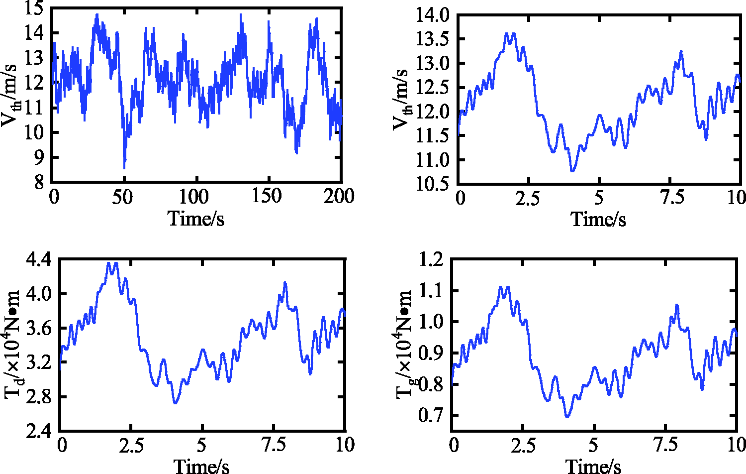
The simulated wind speed of the AR model and the input and output torque.

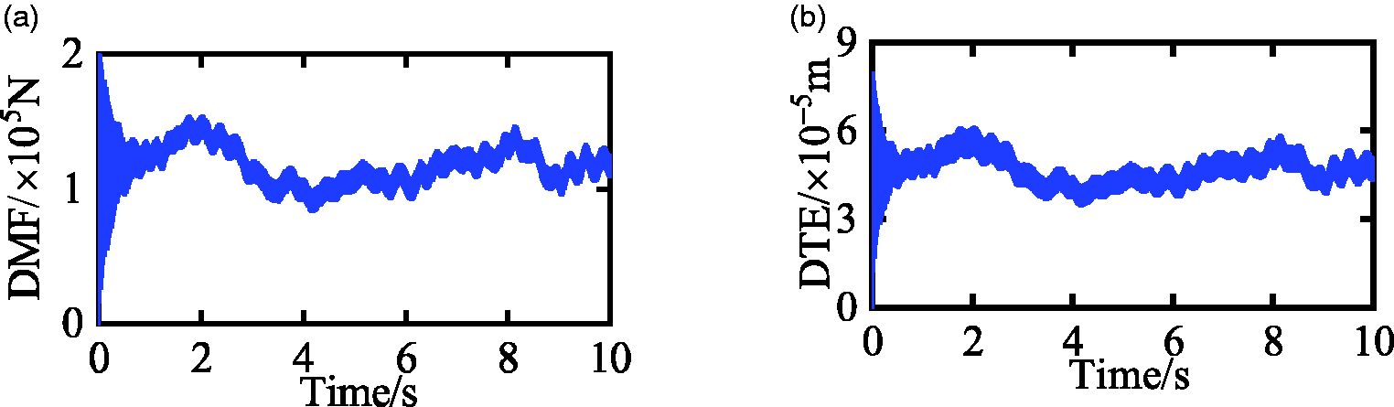
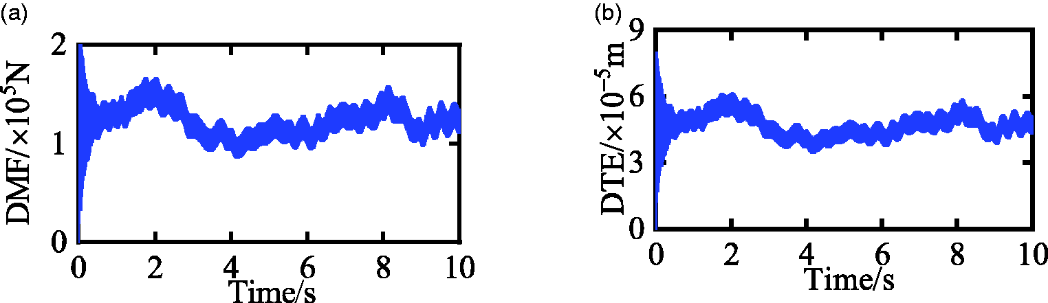
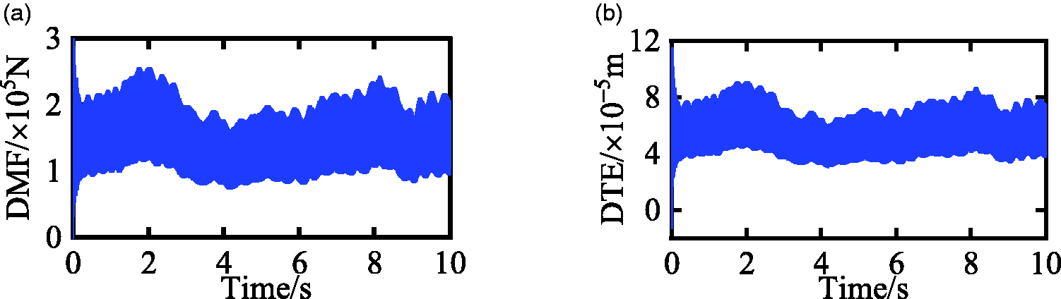
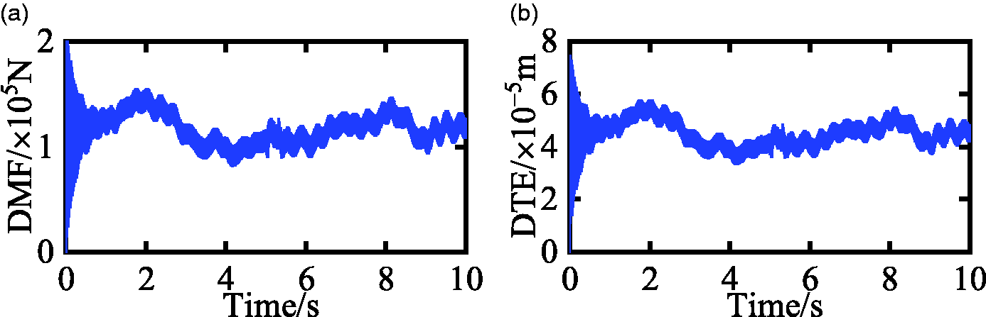
To explore the effect of the friction coefficient on the gear transmission system, the friction coefficient is controlled as a parameter. It can be known from the above analysis that the high-speed-level gear transmission system of the wind turbine is a multi-degree nonlinear dynamic model. Fourth-order Runge-Kutta is used to solve the vibration differential equations of the model. Dynamic mesh force (DMF) and dynamic transmission error are attained as shown in Figures 7 to 9. It is seen that the fluctuation trend of DMF and DTE is similar to wind speed’s fluctuation trend. The response is analyzed at the different friction coefficients of μ = 0, μ = 0.1 and μ = 0.6. It is clearly seen that the vibration amplitude of DMF and DTE increases with the increase of friction coefficient μ. Therefore, the friction coefficient μ makes their amplitude booming.

Figure 7.

The time-domain waveform (μ = 0).

Figure 8.

The time-domain waveform (μ = 0.1).

Figure 9.

The time-domain waveform (μ = 0.6).

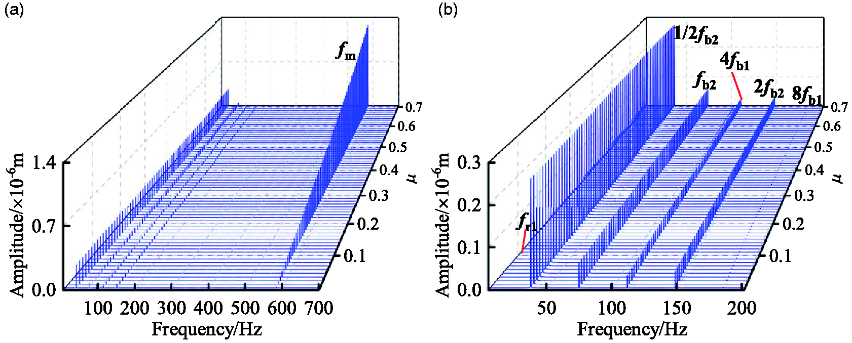
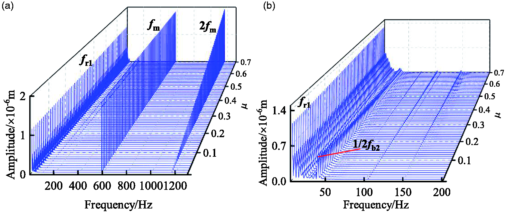
3-D frequency spectra are shown in Figures 10 to 13. The 3-D frequency spectra in x₁ direction are depicted in Figure 10. With increase of friction coefficient, the mesh frequency f_m (f_m=n₁z₁/60 = 583Hz) increases as shown in Figure 10(a). In the spectrum, the amplitude of mesh frequency is the highest. The others are marked in Figure 10(b). The rotational frequency f_r1(f_r1=n₁/60 = 5.95 Hz) also increased with the increase of friction coefficient. When the friction coefficient increases, the amplitude of variable stiffness frequency 4f_b1(f_b1=n₁r₁N₁/60(R₁+r₁) =27.8 Hz) and its frequency multiplication 8f_b1 is not changed. With increase of friction coefficient, the amplitude of variable stiffness frequency f_b2 and its frequency multiplication 2f_b2(f_b2=n₂r₂N₂/60(R₁+r₁) =74Hz) is not changed. When the friction coefficient increases, the frequency amplitude 1/2f_b2 exists a slight fluctuation.

Figure 10.

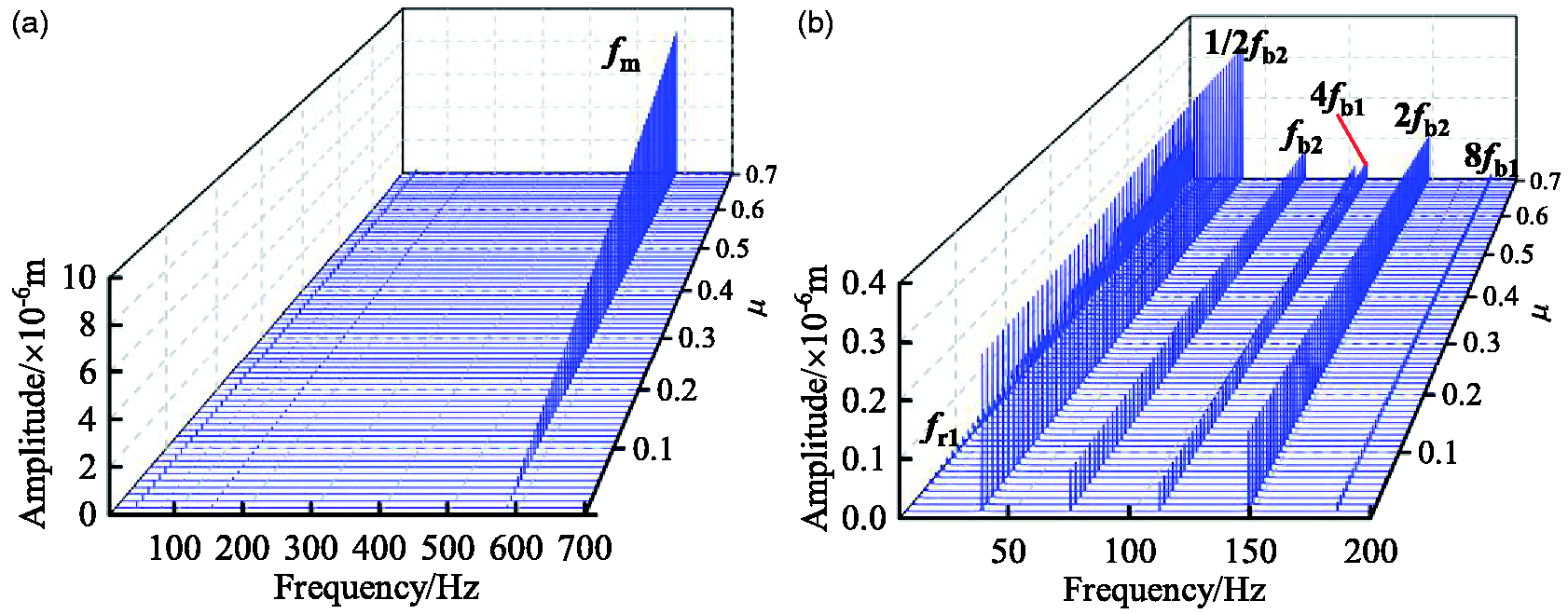
The 3-D frequency spectra in x₁ direction: (a) the 3-D frequency spectrum within the limits of 0–700 Hz, (b) the local image within the limits of 0–200 Hz.

The 3-D frequency spectra in y₁ direction are depicted in Figure 11. It is clearly seen that the frequency component is more complicated than in x₁ direction. The variable trend of frequency is also different. When the friction coefficient increases, the mesh frequency f_m and rotational frequency f_r1 are not changed. The mesh frequency is the largest, and the rotational frequency f_r1 is the second largest. It can be seen that f_r2 appears in the frequency spectrum in y₁ direction. 4f_b1, 8f_b1, f_b2, 2f_b2 amplitude is gradually increasing with the increase of the friction coefficient. The fluctuation of component frequency is exacerbated. The variable trend is first increases, then slowly decreases and finally becomes stable. It illustrates the phenomenon that the same frequency component has different variable laws in a different direction on the gear.

Figure 11.

The 3-D frequency spectra in y₁ direction, (a) the 3-D frequency spectrum within the limits of 0–700 Hz, (b) the local image within the limits of 0–200 Hz.

The 3-D frequency spectra of the bearing in x_b1 direction are shown in Figure 12. It is clearly seen that the mesh frequency f_m and the rotational frequency f_r1 are increased little by little with the increase of the friction coefficient. The mesh frequency is not the largest all the while. Approximately, the amplitude of mesh frequency is the largest within the limits of $\text{μ}\in [0.3,0.7]$ . In other words, the frequency 1/2f_b2 is the largest at µ<0.3 in the spectrum in x_b1 direction.

Figure 12.

The 3-D frequency spectra in x_b1 direction: (a) the 3-D frequency spectrum within the limits of 0–700 Hz, (b) the local image within the limits of 0–200 Hz.

The 3-D frequency spectra of the bearing in y_b1 direction are shown in Figure 13. The mesh frequency is the largest all the while. But the second-largest is not fixed. Approximately, the rotational frequency f_r1 is the second largest at µ<3.5. When µ is greater than 3.5, the frequency 1/2f_b2 is the second largest. The mesh frequency f_m and rotational frequency f_r1 were not changed by the friction coefficient. With the increase of µ, the amplitude increases, including f_b2, 2f_b2, 4f_b1, 8f_b1 and 1/2f_b2.

Figure 13.

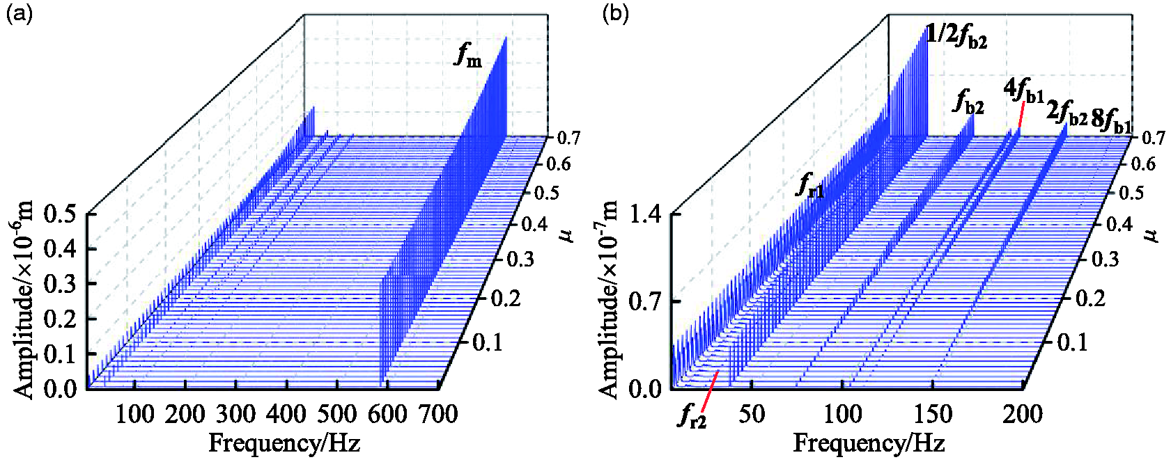
The 3-D frequency spectra in y_b1 direction: (a) the 3-D frequency spectrum within the limits of 0–700 Hz, (b) the local image within the limits of 0–200 Hz.

The vibration response of the gear transmission system is analyzed under different conditions, including three friction coefficients of μ = 0, μ = 0.1 and μ = 0.6. The results are shown in Figures 14 to 16. The vibration response at μ = 0 is depicted in Figure 14. When the friction force does not exist on the gear transmission system (µ=0), the variation trend of displacement in x₁ direction is not matched with the wind speed. But y₁ direction presents a reverse relation. The amplitude of mesh frequency is slight. The frequency 1/2f_b2 is the largest in x direction, including x₁ and x_b1, as depicted in Figure 14(b1) and (b₃). The mesh frequency f_m is the largest in y₁ and y_b1 direction as shown in Figure 14(b2) and (b₄).

Figure 14.

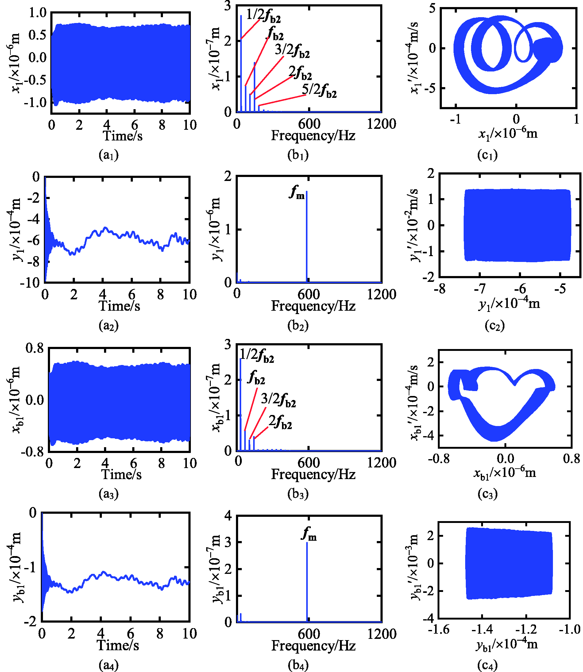
The response of the gear system (μ = 0): a _i represents time domain waveform, b _i represents frequency spectrum, c _i represents phase map (i = 1, 2, 3, 4). i = 1 in x₁ direction, i = 2 in y₁ direction, i = 3 in x_b1 direction, i = 4 in y_b1 direction.

In Figure 15, the vibration response at (µ=0.1) is shown. When the friction force exists, the variable trend of the displacement in x direction presents a positive relationship or called the same variation as the wind load within the limits of 10 s as shown in Figure 6(b). Reversely, y direction trend is a reverse relation with the wind speed. The mesh frequency again becomes the largest frequency in x₁, y₁, y_b1. However, the frequency 1/2f_b2 is the largest in x_b1. The phenomenon can be made mention of Figure 12(a) interpretation. Approximately, the displacement amplitude of x₁ is a hundredfold increase and x_b1 is a tenfold increase than no friction. Thereupon, the phase diagram trajectory becomes wide. The phase diagram trajectory is split. It is clearly seen that the trajectory comprises several closed regular elliptical rings. It can be deduced that the gear system motion state is a stable periodic motion.

Figure 15.

The response of the gear system (μ = 0.1): a _i represents time domain waveform, b _i represents frequency spectrum, c _i represent phase map (i = 1, 2, 3, 4). i = 1 in x₁ direction, i = 2 in y₁ direction, i = 3 in x_b1 direction, i = 4 in y_b1 direction.

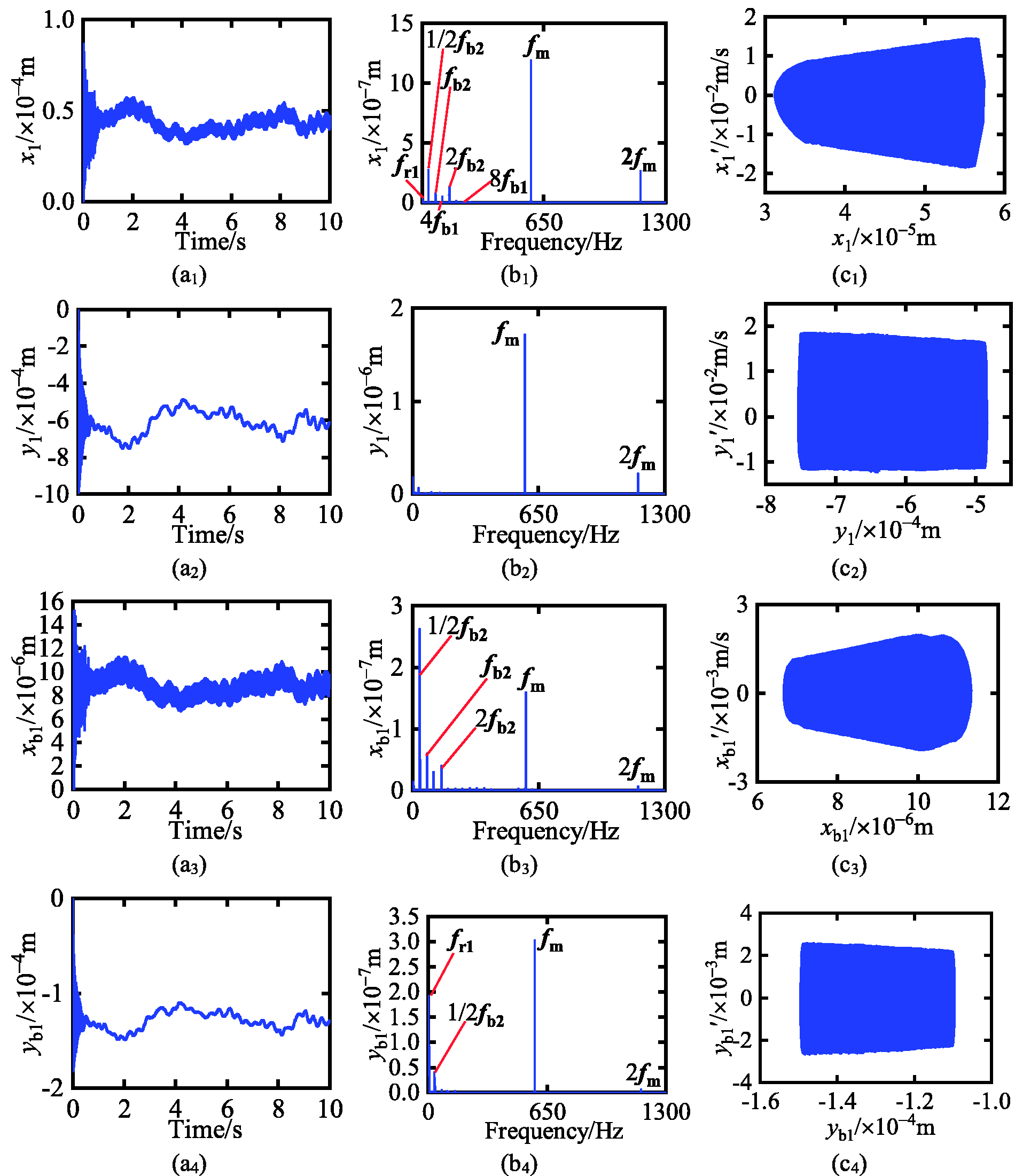
When the friction coefficient further increases μ = 0.6, the variable trend of displacement amplitude becomes steeper than before in Figure 16(a _i ). The mesh frequency f_m and its frequency multiplication 2 f_m are bigger than before in x₁ and y₁ in Figure 16(b1) and (b₂).

Figure 16.

The response of the gear system (μ = 0.6): a _i represents time domain waveform, b _i represents frequency spectrum, c _i represent phase map (i = 1, 2, 3, 4). i = 1 in x₁ direction, i = 2 in y₁ direction, i = 3 in x_b1 direction, i = 4 in y_b1 direction.

Dynamic response of the system with electromagnetic torque disturbance

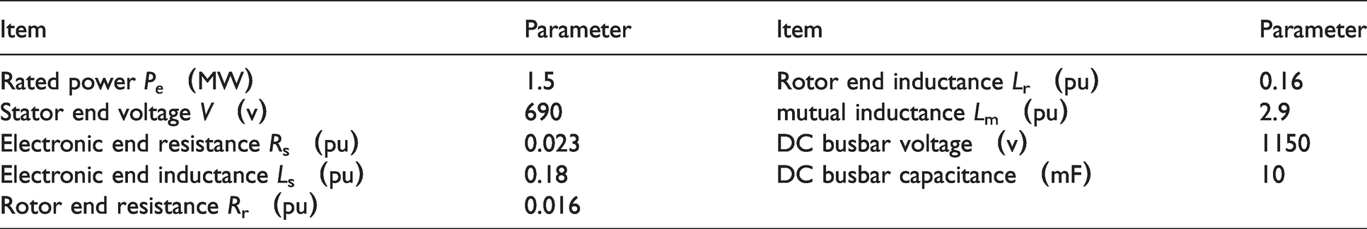
On the basis of the time-varying wind load mentioned in the Dynamic response of the system with time-varying wind load section, the electromagnetic torque disturbance can be solved by the DFIG model of the wind turbine. The parameters of DFIG are shown in Table 3. If a small drop in the voltage grid appears, the output torque end of the gear transmission system will produce a fluctuation called electromagnetic torque disturbance. This fluctuation can be calculated by the Matlab/Simulink model of DFIG. The voltage drop starts at 5 s and lasts for 200 ms. If the voltage grid drops to 90% of the current-voltage, the output torque T_g is shown in Figure 17(b).

Table 3.

Parameter of DFIG power system.

Item	Parameter	Item	Parameter
Rated power Pe （MW）	1.5	Rotor end inductance Lr （pu）	0.16
Stator end voltage V （v）	690	mutual inductance Lm （pu）	2.9
Electronic end resistance Rs （pu）	0.023	DC busbar voltage （v）	1150
Electronic end inductance Ls （pu）	0.18	DC busbar capacitance （mF）	10
Rotor end resistance Rr （pu）	0.016

Figure 17.

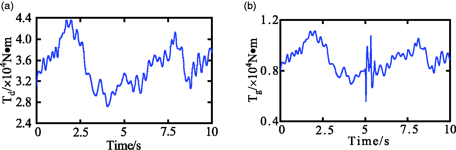
The input and output torque.

On the basis of the Dynamic response of the system with time-varying wind load section, the input torque T_d remains unchanged as shown in Figure17(a). After substituting equation (34), the differential equation is solved by fourth-order Runge-Kutta. Considering the time-varying wind load and electromagnetic torque disturbance, the dynamic response of the system can be given. DMF and DTE of the system are respectively shown in Figures 18 to 20 with different friction coefficient μ. According to the figures, there is the same trend fluctuation as T_g. With increase of friction coefficient, the electromagnetic torque disturbance is gradually covered up by the influence of the friction coefficient.

Figure 18.

The time-domain waveform (μ = 0).

Figure 19.

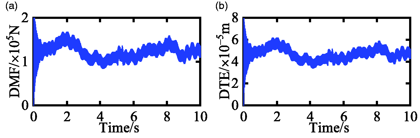
The time-domain waveform (μ = 0.1).

Figure 20.

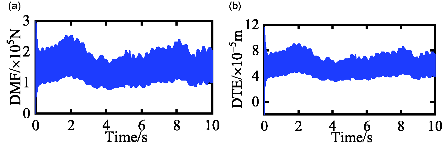
The time-domain waveform (μ = 0.6).

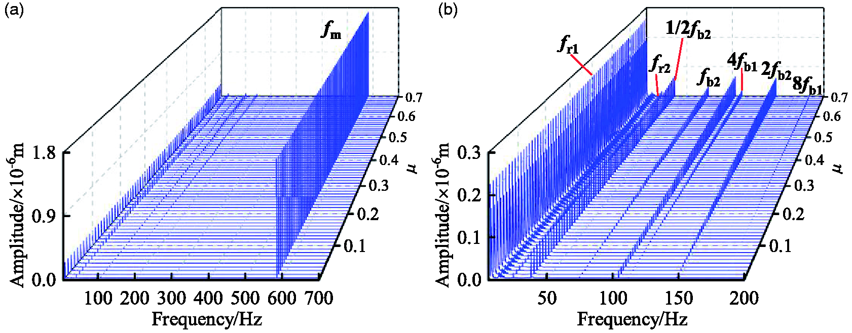
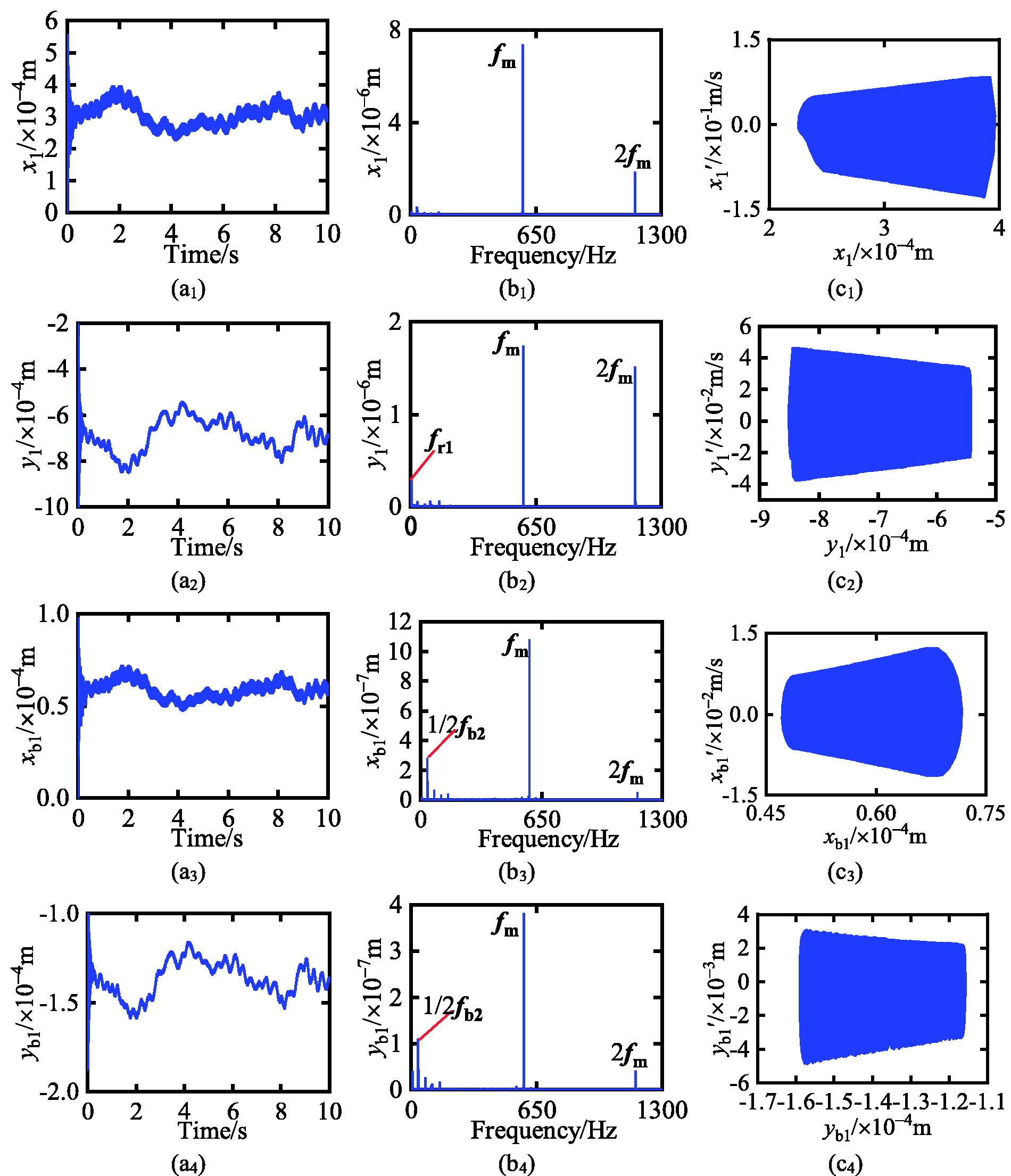
Three-dimensional frequency spectra of gear are described in Figures 21 and 22. Compared with Figure 10, the amplitude variation of frequency constituent f_m and 2 f_m is the same. However, the amplitude of the whole becomes larger due to electromagnetic torque disturbance. The change is the most pronounced in the low frequency. The change is the most pronounced in the low frequency. Frequency doubling appears near f_r1 and the amplitude of f_r1 is bigger than in Figure 10 with increase of friction coefficient. In the vicinity of the low-frequency components, there are different degrees of sidebands. The sidebands of 2f_b2 are the most obvious within the limits of $\text{μ}\in [0.53,0.7]$ . The frequency f_m is still the main frequency component.

Figure 21.

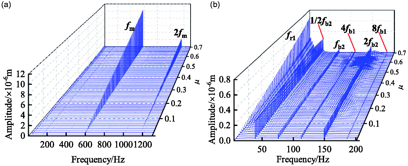
The 3-D frequency spectra in x₁ direction: (a) the 3-D frequency spectrum within the limits of 0–1300 Hz, (b) the local image within the limits of 0–200 Hz.

Figure 22.

The 3-D frequency spectra in y₁ direction: (a) the 3-D frequency spectrum within the limits of 0–1300 Hz, (b) the local image within the limits of 0–200 Hz.

Compared with Figure 11, the amplitude variation of frequency constituent f_m and 2 f_m is the same. But the low-frequency parts are entirely different. The amplitude variation trend of 1/2f_b2 goes from constant to decrease. The effect of electromagnetic torque disturbance on the y₁ direction low-frequency spectrum has a greater influence than in the x₁ direction.

Conclusions

Based on the gear-rotor-bearing transmission system model, in this study the effect of the time-varying wind load and the electromagnetic torque disturbance has been explored. The vibration characteristics and frequency laws are shown in the following:

The vibration displacement variation trend of the gear and bearing is closely related to the wind load variation trend. The gear and bearing’s vibration displacement in the horizontal direction (x) is similar to the wind load trend. But it is reverse in a vertical direction (y). In the domain frequency without electromagnetic torque disturbance, the frequency component in y direction is more abundant than in the x direction. The law of frequency amplitude variation is different with the increase of the friction coefficient. The mesh frequency is not always the largest frequency amplitude in the spectrum of bearing. The low-frequency component in all directions can be seriously influenced by the friction.

When the output end has electromagnetic torque disturbance, the amplitude of low-frequency parts is bigger than without electromagnetic torque disturbance. It can be seen that sidebands exist near low-frequency parts. When the friction coefficient achieves some value, sidebands are more serious in spectra. This study has found that due to the electromagnetic torque disturbance, frequency fault characteristics are almost certainly present in the low-frequency portion. The study contributes to our deep understanding of the design and diagnosis of the gear system of the wind turbine.