Sage Journals: Discover world-class research

Abstract

This paper explores the application of predictive control methods for actively managing structural vibrations and proposes a model predictive controller based on low-dimensional nonlinear reduced-order functions. By training neural networks to identify and train reduced-order nonlinear functions, the feasibility of this approach in controlling complex structures has been verified. The results indicate that the neural network model accurately predicts dynamic responses of the system, while the designed controller exhibits outstanding performance in vibration control across multiple directions for tower cranes. The enhanced controller achieves faster computation by simplifying the predictive model through extended state-space modeling and neural network retraining. Nevertheless, it maintains satisfactory control effectiveness. This method offers new perspectives on reduced-order control of high-dimensional linear and nonlinear systems and shows potential for further enhancing the computational efficiency of model predictive controllers in future research.

Keywords

structural vibration reduced-order functions system identification active control model predictive control

Introduction

Structural vibration control plays a crucial role in contemporary engineering disciplines, notably aerospace, civil engineering, mechanical manufacturing, and ocean engineering.^1–3 As engineering structures continue to grow in complexity and scale, the effective management of structural vibrations not only ensures the safety and durability of these structures but also directly affects system performance and user comfort.^4,5 Over the past few decades, there has been rapid development in vibration control technology; it has evolved from initial passive control to semi-active control and now encompasses extensively studied active control methodologies.^6,7 Passive control is generally confined to single-input single-output systems with a limited controllable frequency range; moreover, it struggles to adapt to complex and variable external excitations.^8,9 Semi-active control combines the advantages of both passive and active controls by achieving vibration suppression through adjustments in damping or stiffness parameters.¹⁰ Magnetorheological (MR) dampers and piezoelectric materials are commonly used smart materials for semi-active control strategies.^11,12 Despite surpassing passive control in certain aspects, the effectiveness of semi-active control remains somewhat constrained.

With advancements in control theory and actuator technology, active control has garnered extensive attention and undergone in-depth research as a more advanced method for vibration control.¹³ Reina et al.¹⁴ utilized a linear quadratic regulator (LQR) for the active control of automotive suspensions, demonstrating its superiority. Wen et al.¹⁵ designed an active tuned mass damper (ATMD) system based on LQR control algorithms, further extending the application of active control to bridge structures. Additionally, Zhang et al.¹⁶ proposed a proportional-integral-derivative (PID)-LQR hybrid controller, while Huang et al.¹⁷ optimized LQR controllers using Particle Swarm Optimization (PSO), both showing excellent performance under various excitation conditions. These studies collectively indicate that modern control theory has substantial potential for enhancing the robustness of structural vibration control.

Active control of structural vibrations faces significant challenges due to the presence of high-order dynamic equations, which complicate the design of controllers.^18,19 Traditional linear reduced-order methods have proven inadequate in handling nonlinear complex systems and fail to fully address the demands of engineering practice.^20–22

To address these challenges, this paper introduces a neural network model predictive control method based on nonlinear reduced-order functions that accurately predict system response.^23–29 Furthermore, it simplifies multi-step prediction by directly computing the neural network, thereby enhancing controller speed. The effectiveness of the proposed method is demonstrated through validation using a tower crane finite element model, highlighting its potential for active control over complex structures. The main contributions of this study are as follows:

1. A novel nonlinear reduced-order method is proposed that is capable of accurately characterizing the dynamic characteristics of complex structures.

2. A neural network-based multi-step prediction model is developed to improve prediction accuracy and computational efficiency.

3. An improved model predictive control algorithm is designed to enhance the robustness and adaptability of the control system.

4. The effectiveness of the proposed method in controlling complex engineering structural vibrations is validated through a case study on tower cranes.

Reduced-order control system design

Governing equation

Assuming linear elastic deformation of structural members, the system comprising the structure, actuator, sensor, and impact load can be described using the dynamic equation of degrees of freedom:

M \ddot{x} (t) + C \dot{x} (t) + K x (t) = B u (t) + D p (t)

(1)

where

R^{n \times 1}

denotes a matrix with n rows and 1 column. n represents the degrees of freedom of the structure.

\ddot{x}

\dot{x}

, and

x

represent the acceleration, velocity, and displacement vectors of various nodes of the structure, respectively. M, C, and K

\in R^{n \times n}

stand for the mass, damping, and stiffness matrices of the structure in global coordinates. p

\in R^{q \times 1}

is a q-dimensional vector composed of external disturbances encountered during system operation, while D is a matrix influencing the positions of impact loads. u is the vector consisting of active control forces exerted by r actuator systems on the structure system. B

\in R^{n \times r}

is a matrix influencing the positions of active control forces. All variables including

\ddot{x}

\dot{x}

x

u

, and

p

are functions with respect to t (time).

Defining the state variable z in equation (2) as:

z (t) = [\begin{array}{l} x (t) \\ \dot{x} (t) \end{array}]

(2)

The system state equations and output equations can be derived:

{\begin{cases} \dot{z} (t) = A z (t) + E U (t) \\ y (t) = C z (t) \end{cases}

(3)

where

A = [\begin{array}{l} 0 & I \\ - M^{- 1} K & - M^{- 1} C \end{array}]

, I represents the identity matrix,

E = [\begin{array}{l} 0 & 0 \\ M^{- 1} B & M^{- 1} D \end{array}]

U = [\begin{array}{l} u (t) \\ p (t) \end{array}]

, C is the output matrix (assumed to be the identity matrix in this paper), y(t) denotes the output vector and is equal to the state variable z(t). Assuming that the system initiates at time t₀ with state z(t₀), equation (3) provides a solution:

z (t) = e^{A (t - t_{0})} z (t_{0}) + \int_{t_{0}}^{t} e^{A (t - t_{0})} E U (τ) d τ, t \geq t_{0}

(4)

Let T represent the system sampling time, with an initial time t₀ = 0 and t = t₀+kT, k = 0,1,2, $\dots$ . Assuming a constant system input force U within each sampling period. By substituting t=(k+1)T and t₀ = T into equation (5), we obtain the discrete equation of the system with sampling period T:

z [(k + 1) T] = e^{A T} z (k T) + \int_{k T}^{(k + 1) T} e^{A T} E U (k T) d τ, t \geq t_{0}

(5)

To obtain the discrete state-space equations, their simplified form is given by:

{\begin{cases} z (k + 1) = \overset{⌢}{A} z (k) + \overset{⌢}{E} U (k) \\ y (k) = C z (k) \end{cases}

(6)

In the above expression:

\overset{⌢}{A} = e^{A T} \in R^{2 n \times 2 n}

\overset{⌢}{E} = \int_{0}^{T} e^{A T} E d τ \in R^{2 n \times (q + r)}

。

Nonlinear model reduction

As the number of finite element nodes in the structure increases, the structural response converges towards the actual response. However, this also leads to an increase in the value of n in equation (6), making it challenging to directly use equation (6) for controller design at very high values of n. Therefore, it becomes necessary to reduce the order of equation (6).

The i-th row of the state-space equation in equation (6) is as follows:

z_{i} (k + 1) = \sum_{j = 1}^{2 n} {\overset{⌢}{A}}_{i j} z_{j} (k) + \sum_{l = 1}^{q + r} {\overset{⌢}{E}}_{i l} U_{l} (k)

(7)

where z_i represents the i-th element of vector z;

{\overset{⌢}{A}}_{i j}

denotes the element at the i-th row and j-th column of matrix

\overset{⌢}{A}

;

{\overset{⌢}{E}}_{i l}

refers to the element at the i-th row and l-th column of matrix

\overset{⌢}{E}

; and U_l signifies the element in the l-th column of matrix U.

In equation (7), it ensures that total force acting on each node is limited, resulting in a finite value for $\sum_{l = 1}^{q + r} {\overset{⌢}{E}}_{i l} U_{l} (k)$ . Meanwhile, $z_{i} (k + 1)$ is also finite, implying finiteness for $\sum_{j = 1}^{2 n} {\overset{⌢}{A}}_{i j} z_{j} (k)$ as well. Therefore, a summation function exists on the right-hand side of equation (7). There exists a function f_i such that:

z_{i} (k + 1) = f_{i} [z_{1} (k), z_{2} (k), \dots, z_{2 n} (k), U_{1} (k), U_{2} (k), \dots, U_{q + r} (k)]

(8)

In equation (8), the function f_i depends on both z(k) and U(k). All variables, including

z_{1} (k)

z_{2} (k)

\dots

z_{2 n} (k)

and

U_{1} (k), U_{2} (k), \dots, U_{q + r} (k)

are time-dependent functions, therefore, there exists:

z_{i} (k + 1) = g_{i} (t)

(9)

where

g_{i}

represents the function of time.

By selectively removing a small number of elements from z(k) and U(k), denoted by quantities s and v respectively, while ensuring that these elements have unique solutions in time, equation (9) can be transformed into:

z_{i} (k + 1) = g_{i} {t [z_{1}^{'} (k), z_{2}^{'} (k), \dots, z_{s}^{'} (k), U_{1}^{'} (k), U_{2}^{'} (k), \dots, U_{v}^{'} (k)]}

(10)

In equation (10),

z_{1}^{'} (k), z_{2}^{'} (k), \dots, z_{s}^{'} (k), U_{1}^{'} (k), U_{2}^{'} (k), \dots, U_{v}^{'} (k)

are respectively taking out elements from z(k), U(k) that meet requirements. These variables also function independently over time. Then equation (10) can be substituted by:

z_{i} (k + 1) = h_{i} [z_{1}^{'} (k), z_{2}^{'} (k), \dots, z_{s}^{'} (k), U_{1}^{'} (k), U_{2}^{'} (k), \dots, U_{v}^{'} (k)]

(11)

where

h_{i}

represents the function of

z_{1}^{'} (k), z_{2}^{'} (k), \dots, z_{s}^{'} (k), U_{1}^{'} (k), U_{2}^{'} (k), \dots, U_{v}^{'} (k)

The corresponding row of equations in the state space equation of $z_{1}^{'} (k + 1), z_{2}^{'} (k + 1), \dots, z_{s}^{'} (k + 1)$ in equation (6) is extracted and combined as follows:

{\begin{cases} z_{1}^{'} (k + 1) = h_{1} [z_{1}^{'} (k), z_{2}^{'} (k), \dots, z_{s}^{'} (k), U_{1}^{'} (k), U_{2}^{'} (k), \dots, U_{v}^{'} (k)] \\ z_{2}^{'} (k + 1) = h_{2} [z_{1}^{'} (k), z_{2}^{'} (k), \dots, z_{s}^{'} (k), U_{1}^{'} (k), U_{2}^{'} (k), \dots, U_{v}^{'} (k)] \\ ⋮ ⋮ \\ z_{s}^{'} (k + 1) = h_{s} [z_{1}^{'} (k), z_{2}^{'} (k), \dots, z_{s}^{'} (k), U_{1}^{'} (k), U_{2}^{'} (k), \dots, U_{v}^{'} (k)] \end{cases}

(12)

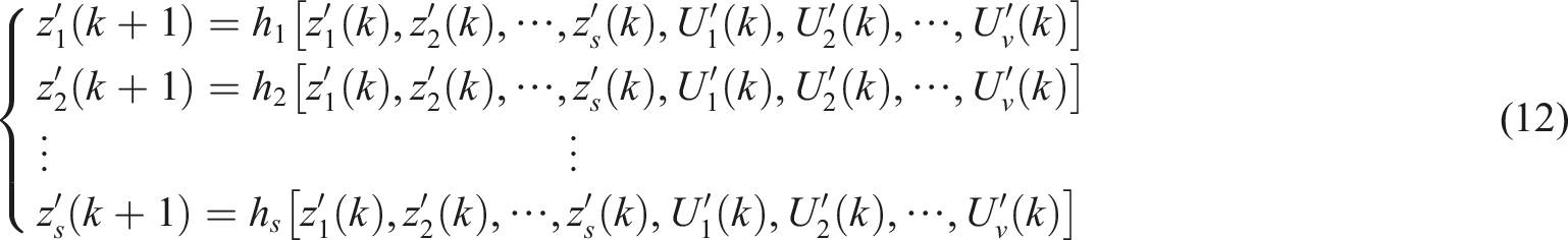
Equation (12) expressed in vector form:

z^{'} (k + 1) = H [z^{'} (k), U_{v}^{'} (k)]

(13)

In equation (13),

z^{'} (k) = {[z_{1}^{'} (k), z_{2}^{'} (k), \dots, z_{s}^{'} (k)]}^{T}

U^{'} (k) = {[U_{1}^{'} (k), U_{2}^{'} (k), \dots, U_{v}^{'} (k)]}^{T}

, H represents the corresponding nonlinear mapping. Based on the aforementioned calculations, it can be observed that there exists a nonlinear mapping function that establishes a connection between the extracted discrete state variables. Equation (13) represents the corresponding equation for the nonlinear discrete state space.

Neural network system identification

The backpropagation (BP) neural network serves as an effective tool for accurately fitting the nonlinear function mapping relationship H corresponding to equation (13). In order to obtain the mapping relationship of the unknown function H, the neural network requires utilizing $U^{'} (k - 1)$ and $z^{'} (k - 1)$ from the (k-1)-th sampling as inputs, while using $z^{'} (k)$ from the k-th sampling as a reference for output in Figure 1. This figure depicts the process of obtaining the total error function J through neural network identification.

U_{n e t} (k - 1) = {[U_{1}^{'} (k - 1), U_{2}^{'} (k - 1), \dots, U_{v}^{'} (k - 1), z_{1}^{'} (k - 1), z_{2}^{'} (k - 1), \dots, z_{s}^{'} (k - 1)]}^{T}

(14)

Y_{d} = z^{'} (k) = {[z_{1}^{'} (k), z_{2}^{'} (k), \dots, z_{s}^{'} (k)]}^{T}

(15)

In equations (14) and (15),

U_{n e t} (k - 1)

is the input to the neural network during the (k-1)-th sampling, while Y_d denotes the reference output of the neural network during the k-th sampling. The neural network adapts its connection weights through training, which is briefly elucidated in this paper; for detailed principles, please refer to Reference 30.

Figure 1.

Schematic diagram of neural network identification.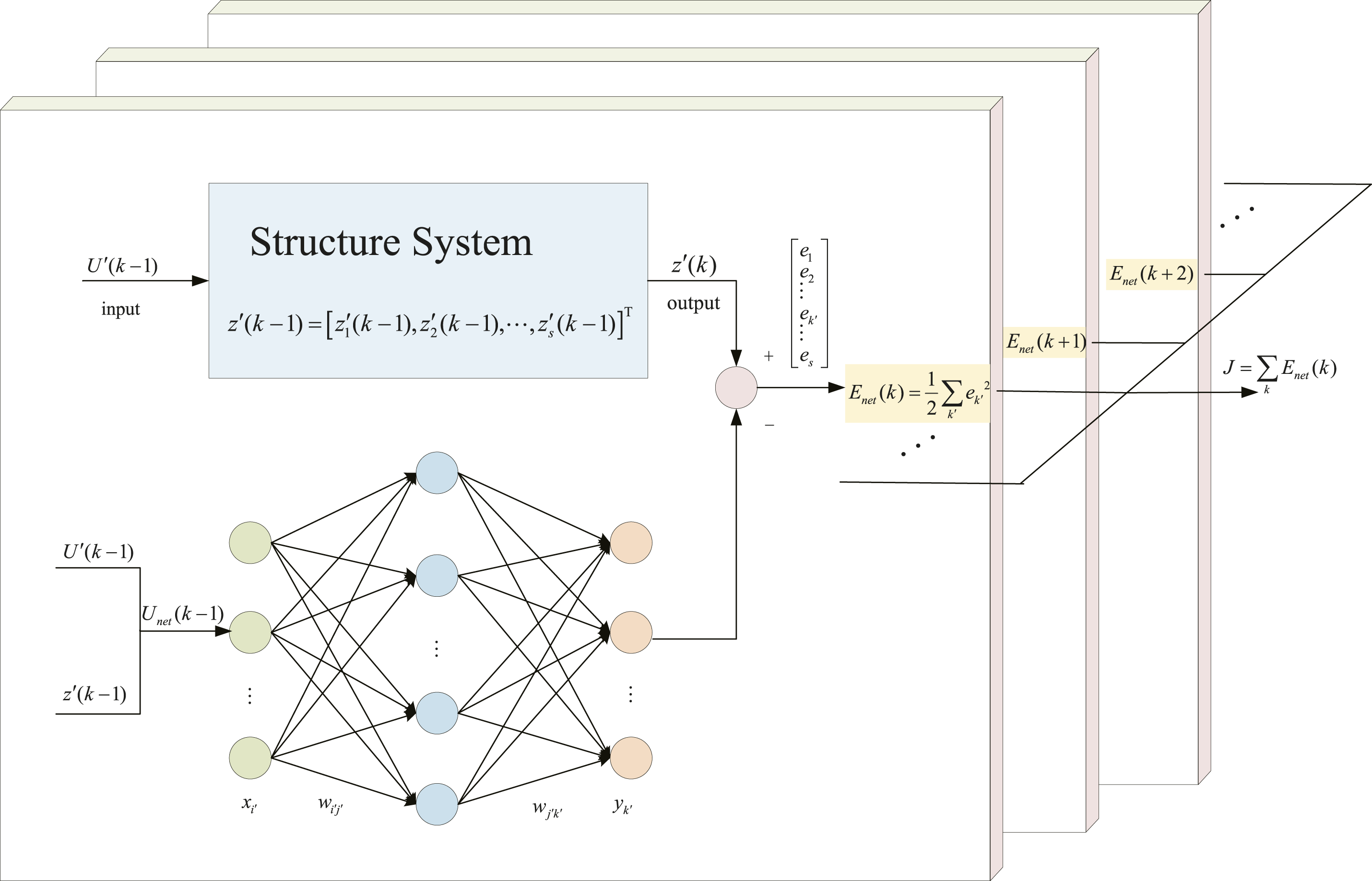

The value at hidden layer node $j^{'}$ , denoted as $x_{j^{'}}$ , is given by:

x_{j^{'}} = f_{n e t} [\sum_{i^{'}} w_{i^{'} j^{'}} x_{i^{'}}]

(16)

f_{n e t} (x_{n e t}) = \frac{1}{1 + e^{- x_{n e t}}}

(17)

In equation (16), the value of

x_{i^{'}}

represents the

i^{'}

-th node in the input layer. Within the context of neural network training discussed in this paper,

x_{i^{'}}

denotes the

i^{'}

-th element of the vector U_net, while

w_{i^{'} j^{'}}

signifies the weight associated with the

j^{'}

-th hidden layer node corresponding to the

i^{'}

-th input node. Additionally, f_net is the nonlinear activation function defined by its mapping relationship in equation (17).

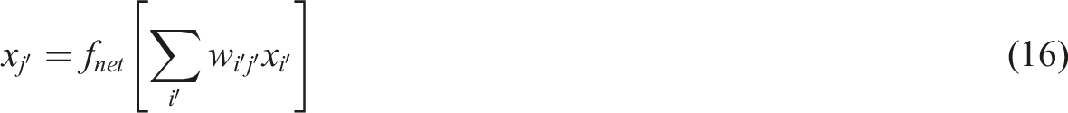
The output of the $k^{'}$ -th output layer neuron is:

y_{k^{'}} = \sum_{j^{'}} w_{j^{'} k^{'}} x_{j^{'}}

(18)

where

x_{j^{'}}

represents the value of the

j^{'}

-th hidden layer node, and

w_{j^{'} k^{'}}

represents the weight of the

k^{'}

-th output layer node corresponding to the

j^{'}

-th hidden layer node.

Let $E_{n e t} (k)$ be defined as the objective function of the network at the k-th sampling, which is expressed as the Euclidean norm between neuron output and reference output. Meanwhile, $e_{k^{'}}$ refers to the discrepancy between neural network output and actual system output.

E_{n e t} (k) = \frac{1}{2} {\sum_{k^{'}} (y_{d k^{'}} - y_{k^{'}})}^{2} = \frac{1}{2} {\sum_{k^{'}} e_{k^{'}}}^{2}

(19)

where

y_{d k^{'}}

is the reference output corresponding to the

k^{'}

-th output layer neuron in Y_d. The overall objective function is formulated as follows:

J = \sum_{k} E_{n e t} (k)

(20)

where J represents the overall performance metric for neural network training. The algorithm determines its completion based on the condition

J \leq ε

, where

ε

is the permissible tolerance with

ε > 0

. The weight update process in the network is as follows:

{\begin{cases} w_{i^{'} j^{'}} (k + 1) = w_{i^{'} j^{'}} (k) + α [w_{i^{'} j^{'}} (k) - w_{i^{'} j^{'}} (k - 1)] - η \frac{\partial E_{n e t} (k)}{\partial w_{i^{'} j^{'}} (k)} \\ w_{j^{'} k^{'}} (k + 1) = w_{j^{'} k^{'}} (k) + α [w_{j^{'} k^{'}} (k) - w_{j^{'} k^{'}} (k - 1)] - η \frac{\partial E_{n e t} (k)}{\partial w_{j^{'} k^{'}} (k)} \end{cases}

(21)

where

α

represents the learning rate coefficient, and

η

is the momentum coefficient.

Predictive controller design

Based on the above derivation, it can be inferred that neural networks have the capability to approximate equation (13) through offline data training. Consequently, they enable prediction of future system responses within a certain number of steps based on the recursive relationship of the difference equation, rendering them suitable for model predictive control.

z_{n e t}^{'} (k + N p) = H_{n e t} [\dots H_{n e t} [H_{n e t} [z^{'} (k), U^{'} (k)], U^{'} (k + 1)] \dots]

(22)

where

z_{n e t}^{'} (k + N p)

represents the predicted system state by the neural network after Np steps.

The concept of rolling optimization in the controller is illustrated in Figure 2. The control horizon, defined as Nc, starts from time k with an initial state of $z^{'} [k]$ . Rolling optimization control involves solving an optimization problem within the prediction horizon to determine the optimal control sequence $U^{'} [k], U^{'} [k + 1 | k]$ , $, \dots, U^{'} [k + N c | k]$ . Utilizing the offline identified neural network model, the state value $z_{n e t}^{'} [k + 1 | k]$ $, \dots, z_{n e t}^{'} [k + N p | k]$ is computed under this control sequence. After completing control prediction and model computation, only the control $U^{'} [k]$ is implemented in the system while discarding the remaining portion of the control sequence. The objective function for rolling optimization, as defined in equation (23), represents the optimal performance index:

J_{p} = \frac{1}{2} z^{'} {(N p)}^{T} S z^{'} (N p) + \frac{1}{2} \sum_{k = 0}^{N p - 1} [z^{' T} (k) Q z^{'} (k) + U^{' T} (k) R U^{'} (k)]

(23)

In the performance index function, S, Q denotes the weighting coefficients for state variables while R represents the weighting coefficient for control inputs. The relative emphasis between state regulation precision and control energy consumption in the optimization process can be systematically tuned by adjusting the values of S, Q, and R parameters. By substituting

z_{n e t}^{'}

for

z^{'}

during the solution process, the predicted value of the optimal performance index J_p, denoted as J_pnet, can be obtained in equation (24).

{J_{p}}_{n e t} = \frac{1}{2} z_{n e t}^{'} {(N p)}^{T} S z_{n e t}^{'} (N p) + \frac{1}{2} \sum_{k = 0}^{N p - 1} [z_{n e t}^{' T} (k) Q z_{n e t}^{'} (k) + U^{' T} (k) R U^{'} (k)]

(24)

Figure 2.

Basic principles of predictive controller.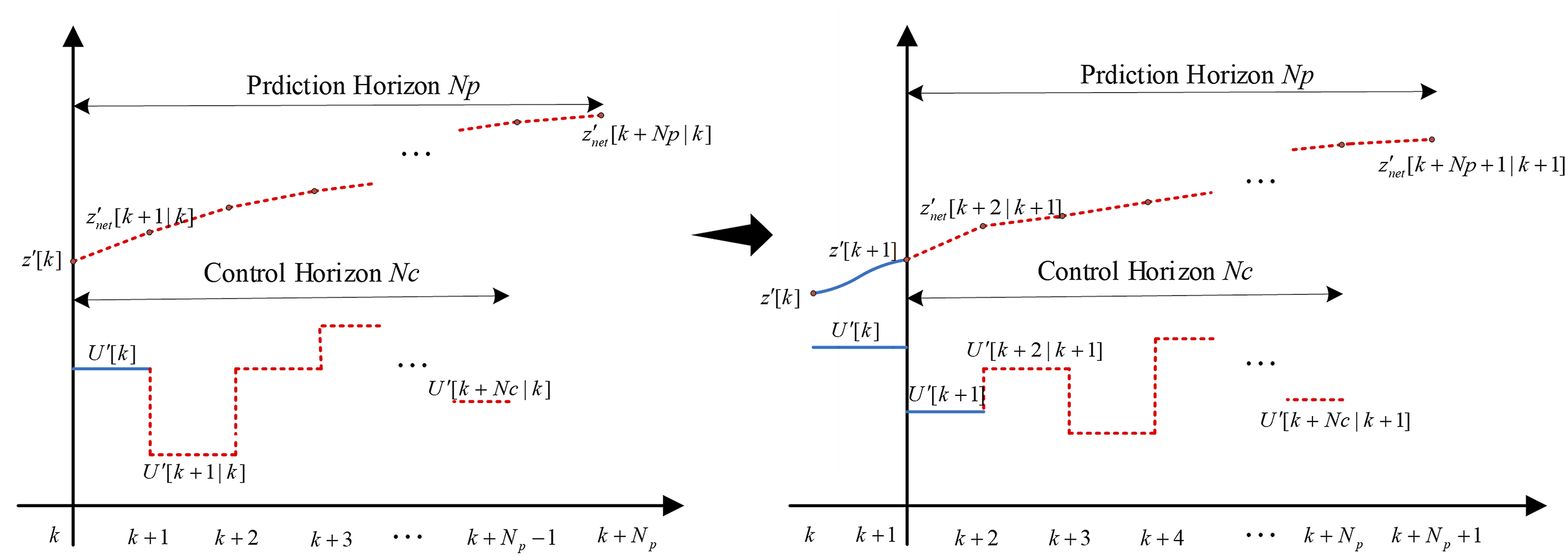

The minimization of J_pnet can be accomplished by using the PSO algorithm, which originates from the investigation of bird flock foraging behavior. PSO is a stochastic search algorithm that relies on population collaboration and enables rapid convergence towards the minimum value of equation (24).

Intelligent reduced-order control architecture for structural systems

The computational flow diagram of the entire reduced-order control system is illustrated in Figure 3. Function $H$ represents the reduced-order function derived from the discrete state-space equation of the system, which serves as a prediction function in predictive control. To obtain this function, the neural network is employed during the offline phase to identify the structural system, resulting in the neural network identification function $H_{n e t}$ . The dataset required for neural network training, denoted as $H_{n e t}$ , is composed of stimulus signals $U^{'} (k)$ and the corresponding structural response data $z^{'} (k)$ .

Figure 3.

Block diagram of reduced-order predictive control system based on neural network.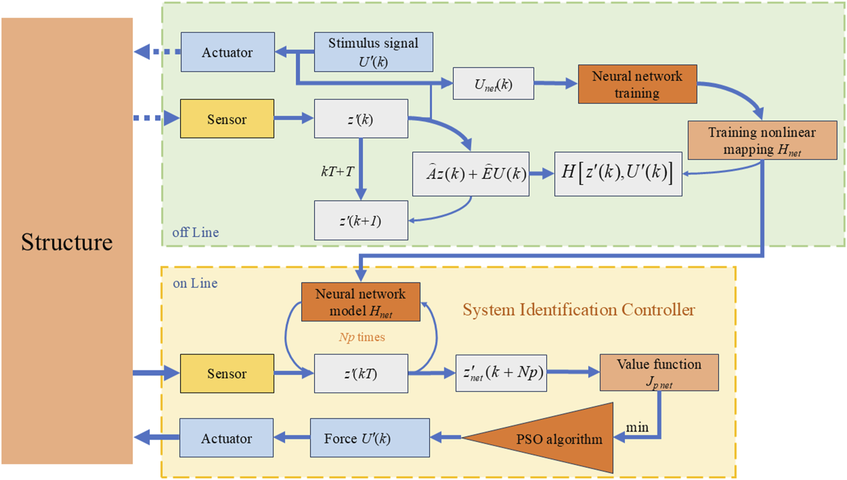

In the actual control process, the neural network-derived mapping H_net, trained offline, approximates the original nonlinear function H, thereby serving as the predictive function. During the online control phase, sensor-acquired data undergoes Np iterations through $H_{n e t}$ for prediction $z_{n e t}^{'}$ . Based on these predictions, the value function $J_{P n e t}$ is calculated. The control system continuously adjusts the input value $U^{'} (k)$ utilizing a PSO algorithm to search for the $U^{'} (k)$ that minimizes $J_{P n e t}$ . Finally, the optimized $U^{'} (k)$ is input to the structure via an actuator, forming a closed-loop control system.

Numerical example

System description

Tower cranes are essential in various engineering projects; however, their susceptibility to vibrations poses significant threats to safety and performance. Despite the high cost associated with active control methods, studying them is important for improving crane safety.

In this study, a finite element model of a tower crane is utilized to validate the proposed method, employing 3D beam and shell elements. A control simulation environment is developed based on this model by incorporating Active Mass Dampers at specific points on the crane to efficiently stabilize it when exposed to external disturbances.

The objective of this research is to demonstrate the effectiveness of the proposed active control method in reducing tower crane vibrations, thereby enhancing safety and efficiency in construction and industrial environments.

The vibration control model of the tower crane, including the Active Mass Damper (AMD) actuator and sensors, is illustrated in Figure 4. The AMD actuator propels as mass block through a piston, utilizing the reaction force of the mass block to apply excitation to the tower crane structure. For a detailed explanation of the underlying principles, please refer to Reference 30. These sensors are responsible for monitoring displacement and velocity at key points. Real-time input forces applied by AMD actuators at specific locations are calculated by the controller. To ensure comprehensive monitoring, sensors are distributed throughout the crane structure. The design of these actuators prioritizes minimal quantity and easy installation. Additionally, various impact loads are imposed on the jib to simulate potential operational disturbances or sudden rope failure.

Figure 4.

Schematic diagram of tower crane vibration control.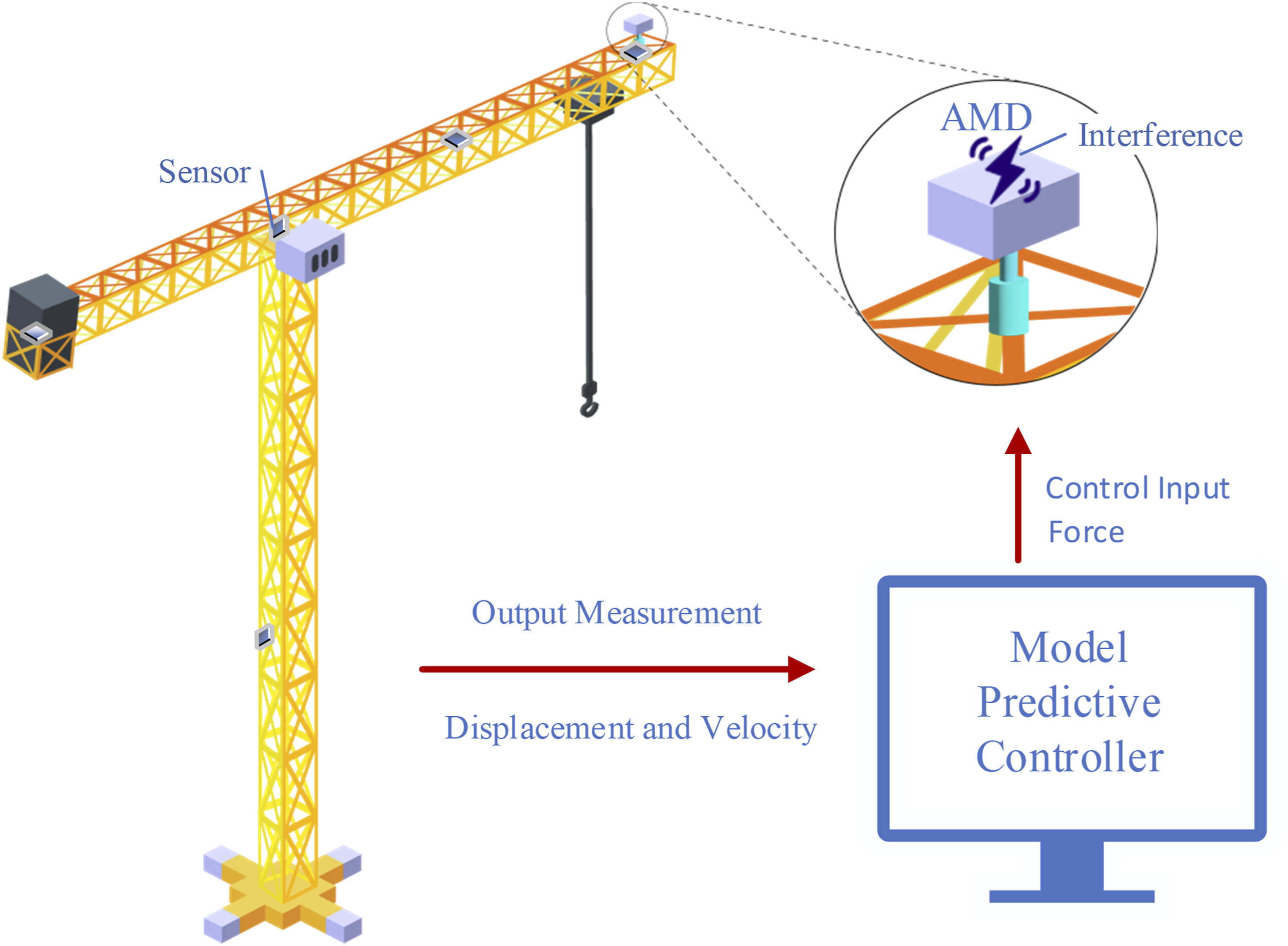

Finite element modeling description

To validate the aforementioned control method, this study conducted finite element modeling research on an ultra-large tower crane located at a construction site. The tower crane under investigation is depicted in Figure 5(a), with its overall dimensions clearly indicated. The total height of the tower crane measures 154.27 m, with a maximum independent height of 146 m. The center distance of the main chord is 3.72 m×3.72 m, while the jib and balance arm have lengths of 77.2 m and 20.55 m, respectively. This particular crane exhibits a truss structure for both the tower and jib end, comprising main chords, horizontal braces, and diagonal braces as illustrated in Figure 5(b) and (c). All main chords, horizontal braces, and diagonal braces of the tower are constructed using square tube structures connected through welding techniques to ensure alignment between their centroids and structural lines depicted in Figure 5(b) and (c). The diagonal braces of the jib end are constructed using circular tube structures. Detailed information regarding cross-sectional dimensions and material properties of these square tubes can be found in Tables 1 and 2.

Figure 5.

Actual photo of the tower crane and schematic diagram of standard section structure.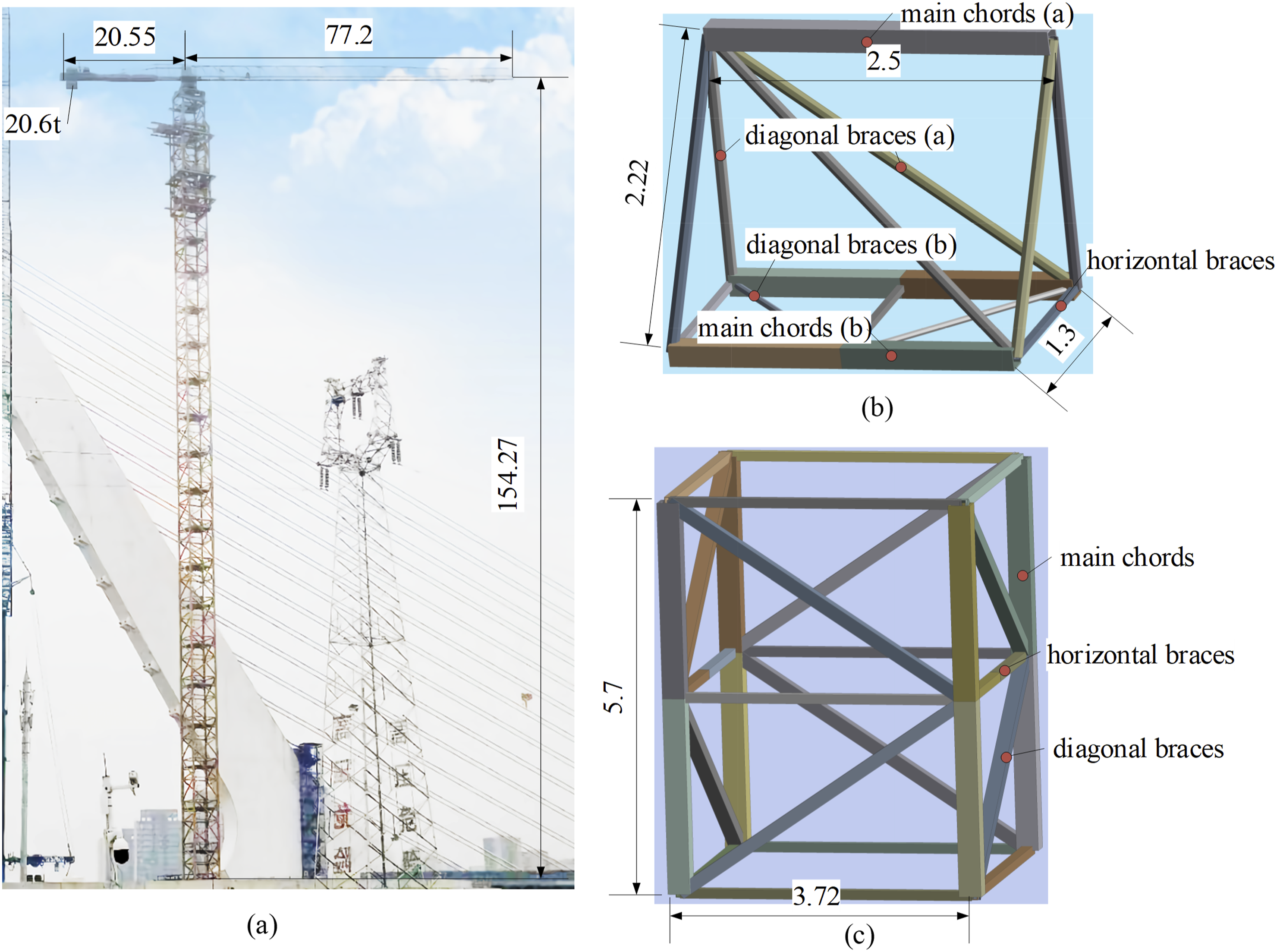

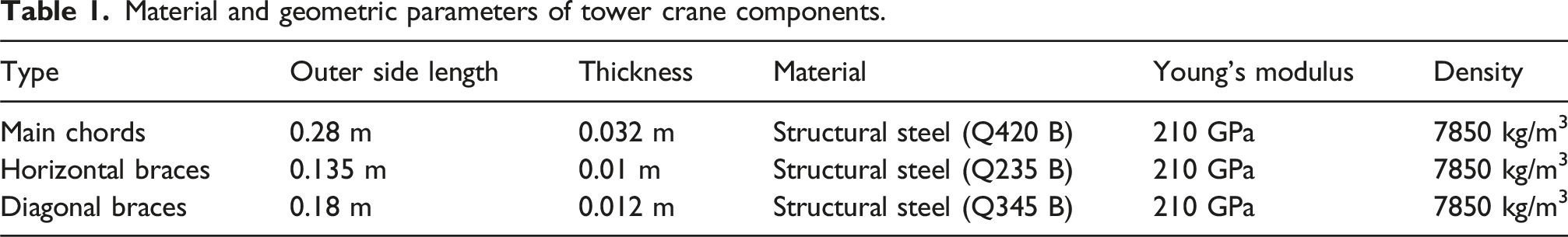
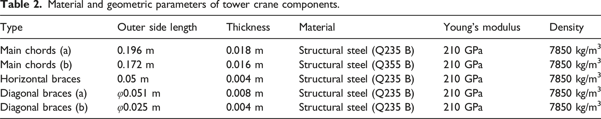
Table 1.

Material and geometric parameters of tower crane components.

Type	Outer side length	Thickness	Material	Young’s modulus	Density
Main chords	0.28 m	0.032 m	Structural steel (Q420 B)	210 GPa	7850 kg/m³
Horizontal braces	0.135 m	0.01 m	Structural steel (Q235 B)	210 GPa	7850 kg/m³
Diagonal braces	0.18 m	0.012 m	Structural steel (Q345 B)	210 GPa	7850 kg/m³

Table 2.

Material and geometric parameters of tower crane components.

Type	Outer side length	Thickness	Material	Young’s modulus	Density
Main chords (a)	0.196 m	0.018 m	Structural steel (Q235 B)	210 GPa	7850 kg/m³
Main chords (b)	0.172 m	0.016 m	Structural steel (Q355 B)	210 GPa	7850 kg/m³
Horizontal braces	0.05 m	0.004 m	Structural steel (Q235 B)	210 GPa	7850 kg/m³
Diagonal braces (a)	φ0.051 m	0.008 m	Structural steel (Q235 B)	210 GPa	7850 kg/m³
Diagonal braces (b)	φ0.025 m	0.004 m	Structural steel (Q235 B)	210 GPa	7850 kg/m³

In the schematic diagram, the tower crane parts are constructed using structural steel, which is characterized by a Young’s modulus of 210 GPa and a density of 7850 kg/m³. The balancing weight is determined to be 20.6 t while considering a natural damping coefficient of 2%.

The accuracy and reliability of the finite element model of a tower crane directly affect the precision of the model analysis results. Due to the inherent complexity in the operational structure of a tower crane, it is not feasible for the calculation model to perfectly align with real-world conditions. In order to strike a balance between convenience and accuracy in analysis and computation, it becomes imperative to simplify both structural aspects and working conditions while assuming correctness and reliability in the finite element model of a tower crane since this assumption significantly influences subsequent model analysis results.

The tower body and upper section are modeled using beam element 188, while the rotary part is simulated using Shell63 element 63. The rigid connection and hinge between them are accurately replicated according to real-world operating conditions. The density of the primary stressed components is adjusted to be 1.1 times their original density, whereas the mass of the tower crane jacket is applied to the top two standard sections and replaced with an equivalent density value. Concentrated masses such as counterweights, mechanisms, and trolley hooks are represented by discrete mass points for simulation purposes.

ANSYS software generates the finite element model, as shown in Figure 6, providing both a comprehensive overview and detailed perspectives. Five critical positions have been meticulously selected for analysis: mid-tower, tower top, balance arm end, mid-boom, and boom end. Each location is equipped with speed and displacement sensors to capture real-time measurements. Subsequently, these sensor readings at each time instance are merged into a vector, that is

z^{'} (k - 1) = {[x 1, x 2, x 3, x 4, x 5, v 1, v 2, v 3, v 4, v 5]}^{T}

(25)

In equation (25), the active control actuator is installed at the distal end of the tower crane’s jib. The force exerted by the actuator on the tower crane is denoted as u1. During the neural network system identification process, no control force is applied; instead, the actuator serves to introduce an excitation force to the tower crane, where u1 corresponds to

U_{v}^{'}

in equation (13).

Figure 6.

Finite element model of tower crane.

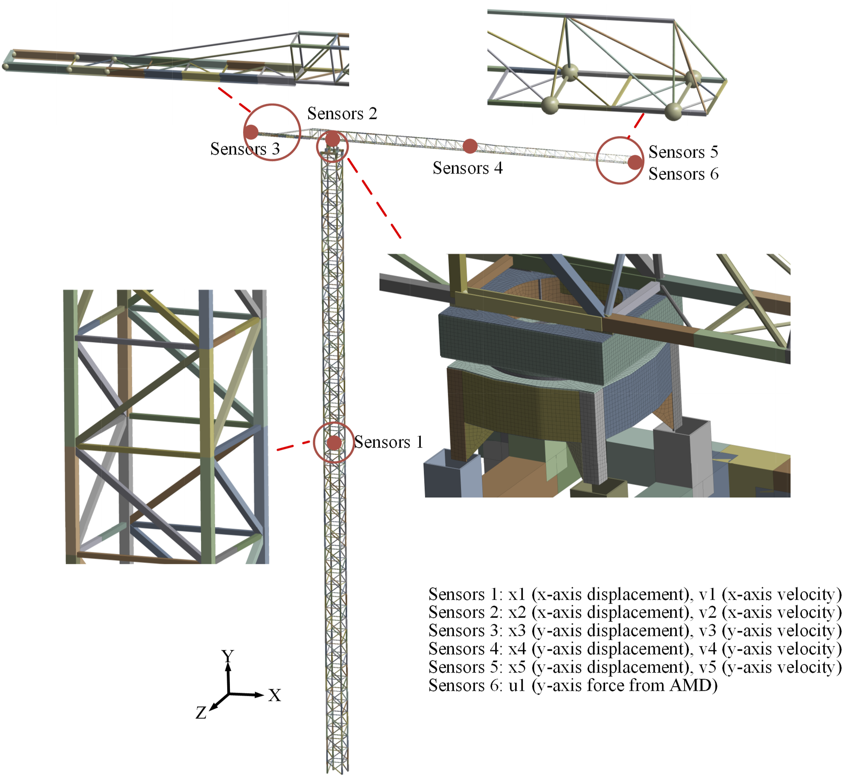
In equation (25), it is recommended to install an active control actuator exclusively at the far end of the jib, where the force exerted by the actuator on the tower crane is denoted as u1. This model should be imported into Adams as a flexible body for accurate data collection via joint simulation using both Adams and Simulink.

Based on the theoretical derivation of optimal input signals in system identification from Reference 30, it is evident that employing Gaussian white noise as the input signal can ensure superior identification outcomes. Assuming a maximum stress capacity of 50000N for the AMD actuator, u1 is designated as a Gaussian white noise signal (with a mean of 0 and variance of 2.25×10⁸), measured in units of N. Here, u1 undergoes changes every 0.1s and is used for neural network system identification purposes. The system sampling time T is set to 0.01s for simulation, with a simulation duration lasting 20s.

In Figure 7, subfigure (a) depicts the magnitude of the input force, while subfigure (b) shows the time-domain curves for x1, x2, x3, x4, and x5 recorded by the displacement sensors. Subfigure (c) displays the time-domain curves for v1, v2, v3, v4, and v5 obtained from velocity sensors.

Figure 7.

Response curves of input force and corresponding sensor positions in the tower crane.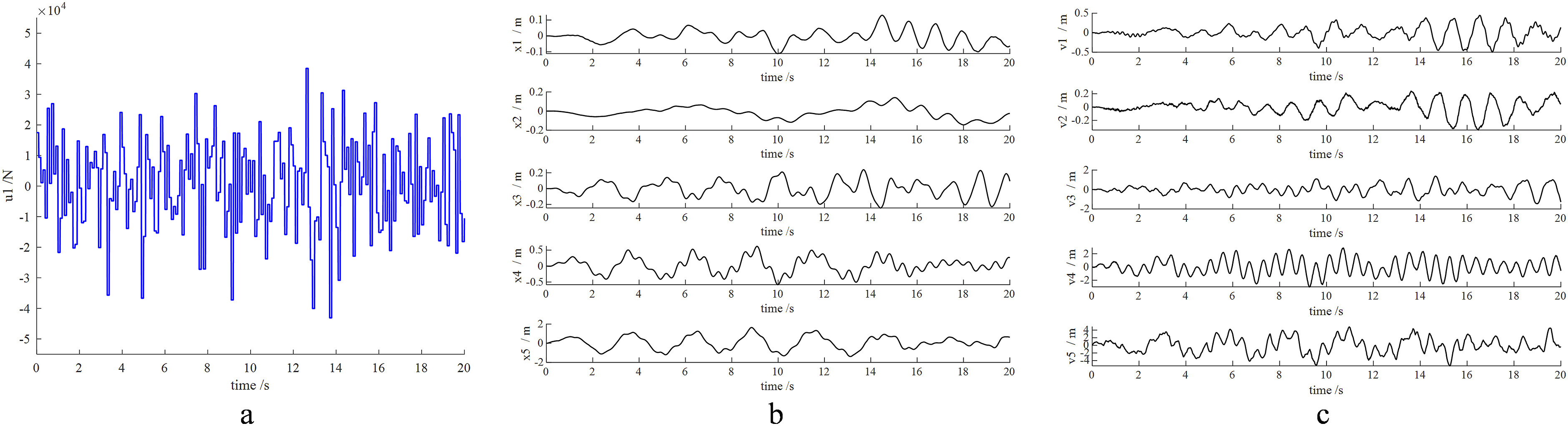

The neural network is trained using u1 as well as the corresponding measurements of x1 to x5 and v1 to v5.

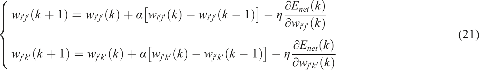
The process of training a neural network is as follows:

1. The number of hidden layer nodes in the neural network is set to 10, and the number of output nodes is also set to 10 (equal to the number of data outputs from the simulation model). The initial values of $w_{i^{'} j^{'}}$ and $w_{j^{'} k^{'}}$ are randomly initialized from a normal distribution with a mean of 0 and a variance of 1.

2. A new vector (totaling 11 elements) is formed by combining the input u1(k-1) from the previous time step (k-1) with $z^{'} (k - 1)$ from equation (25).

3. The newly obtained vector from step 2 serves as the input $U_{n e t} (k - 1)$ to the neural network as per equation (14).

4. The method described in section “Neural network system identification” is employed to calculate the total value function J and continuously adjust the weights $w_{i^{'} j^{'}}$ and $w_{j^{'} k^{'}}$ until J falls below a predefined error threshold $ε$ (in this case, $ε$ = 10^-5). Once this condition is met, it indicates that neural network training has been completed successfully (if desired quality is not achieved, retraining may be necessary).

The tower crane system input u1 in this study is subjected to variations as Gaussian white noise signal, sine wave signal, and step signal with sudden unloading for the purpose of validating the trained neural network model. Here, u1 changes every 0.1 s while maintaining a fixed system sampling time of T = 0.01 s. The data collection method employed for neural network prediction resembles rolling prediction, as shown in Figure 8.

Figure 8.

Illustrates the rolling data acquisition method.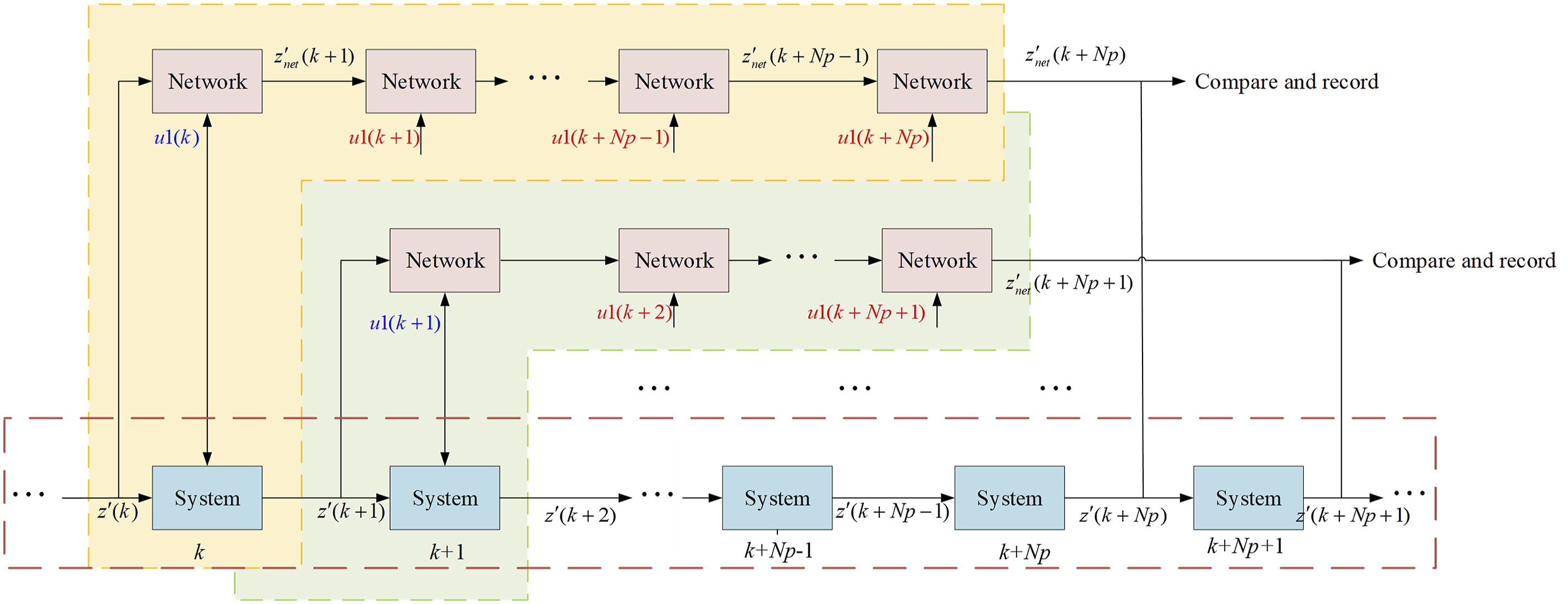

Model of neural network validation

To validate the trained neural network model, the tower crane system underwent testing with a range of input signals, including Gaussian white noise, sinusoidal signals, and step signals (representing sudden unloading). The system was sampled at intervals of 0.1 s.

The three signal types mentioned above represent three typical operational conditions observed in tower cranes. White noise excitation is commonly employed to simulate the random disturbances encountered by tower cranes during operation. Sinusoidal excitation, on the other hand, corresponds to the uneven dynamic loads generated by the motor while lifting or lowering loads. Step excitation specifically refers to impact loads that arise when the lifting rope suddenly breaks during load hoisting operations. These scenarios are extensively investigated by researchers in the field of tower crane engineering.

The data prediction method of the neural network bears resemblance to the rolling prediction used in Model Predictive Control (MPC), enabling real-time comparison between predicted and actual system responses, thereby assessing the model’s accuracy and its potential for effective real-time control.

As shown in Figure 8, the dashed box represents the iterative process of tower crane vibration simulation, while the yellow and green boxes illustrate the iterative procedures within the neural network. The specific data acquisition method is as follows:

1. At time step k, input the system state values and input values into the neural network for Np-step prediction. This advances the simulation time by Np⋅T.

2. Compare the predicted results with the actual system outputs after Np steps and record the discrepancies.

3. Label these two datasets as the neural network’s predicted values and the actual system values at time step k + Np.

4. Repeat steps 1∼3 iteratively to perform rolling data acquisition until the final simulation time.

This rolling data acquisition mimics the predictive steps in MPC. By adopting this method, the neural network’s prediction accuracy at each time step—from the initial prediction to the end of the simulation—is systematically recorded during tower crane vibration analysis.

Input of Gaussian white noise signals

Figure 9 illustrates the prediction results of the neural network for a Gaussian white noise input signal (mean 0, variance 10^8). The predictions are compared with actual system outputs for different horizons of 1, 10, 20, and 30 steps.

Figure 9.

Neural network prediction results under Gaussian white noise signal.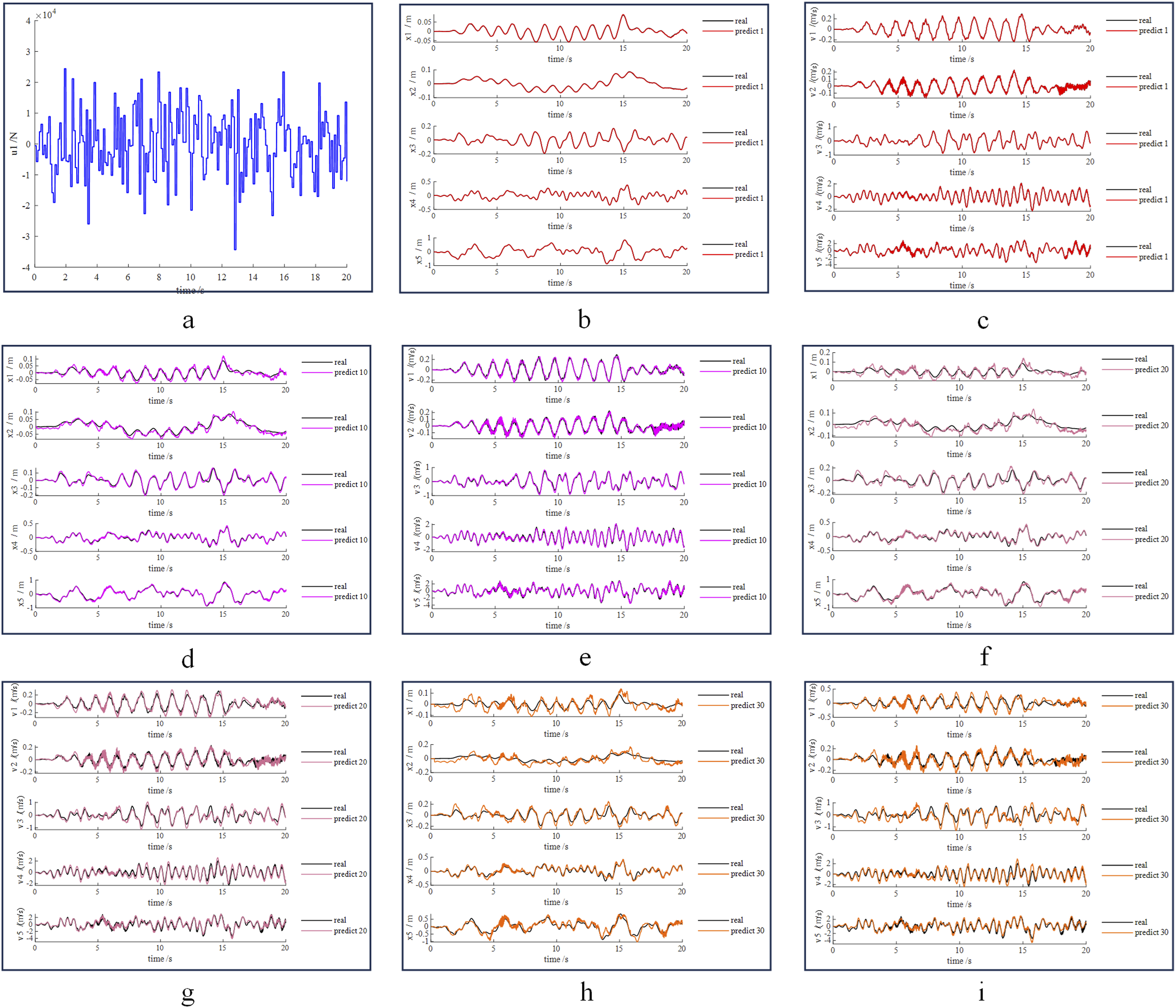

Accuracy levels vary across different prediction horizons, with short-term predictions (1 step) demonstrating excellent accuracy for all variables and exhibiting nearly overlapping predicted and actual curves. Medium-term predictions (10–20 steps) begin to show slight divergence, especially for variables x1 and x2, accompanied by increased noise in the predicted curves while maintaining overall accurate trends. Long-term predictions (30 steps) exhibit larger deviations in amplitude predictions for most variables, particularly at peak and valley points. However, the main vibration frequencies remain consistent with the actual curves, indicating precise prediction of dominant low-frequency vibrations of the tower crane. Notably, even at longer horizons, variables x4, x5, v4, and v5 maintain high prediction accuracy.

Input of sinusoidal signals

The prediction results of the neural network for a sine wave input signal (amplitude 20000, frequency π) are illustrated in Figure 10. A comparative analysis is conducted between the predictions and actual system outputs across different horizons, including 1, 10, 20, and 30 steps.

Figure 10.

The neural network prediction results when u1 is a sine signal.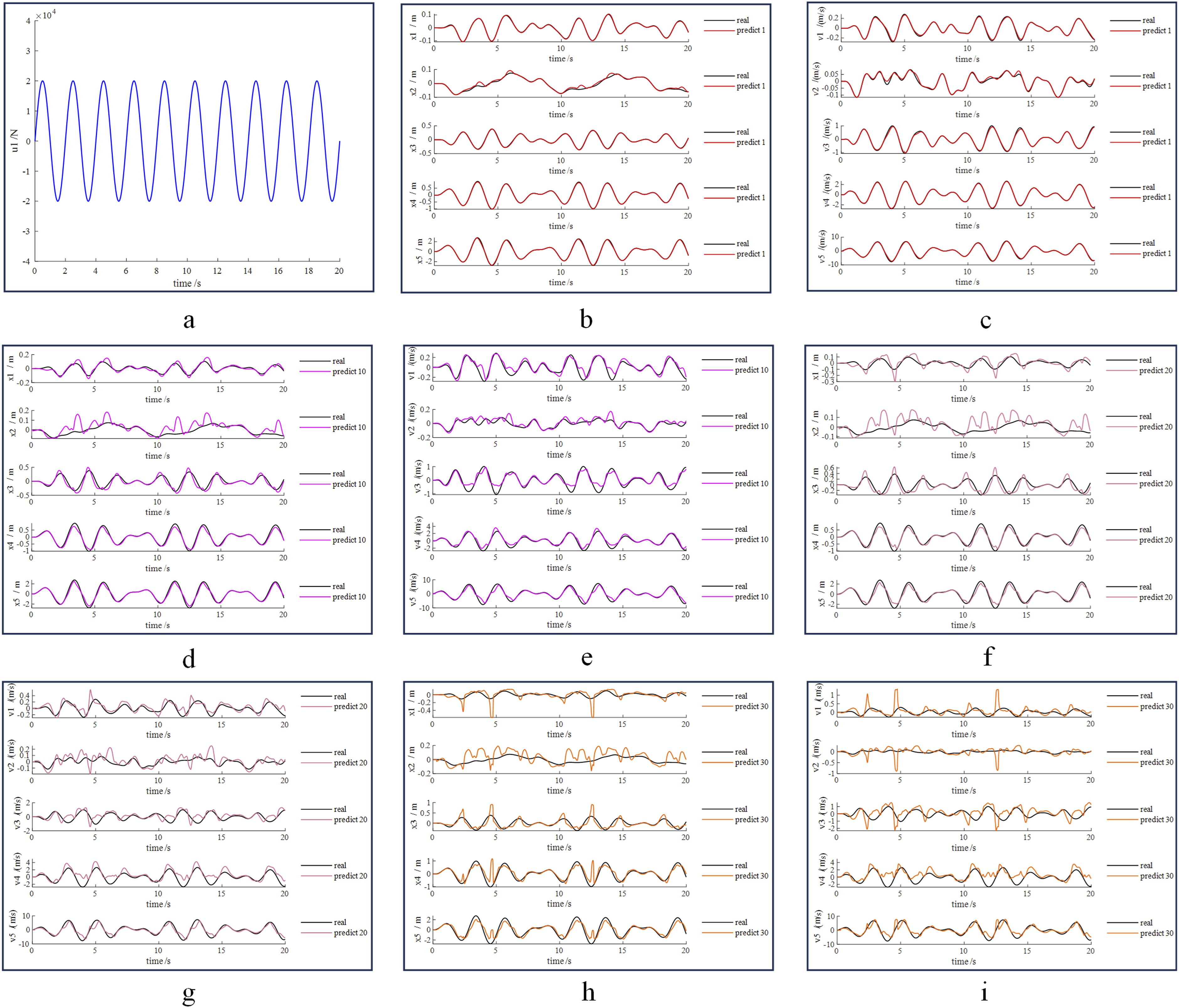

Across different prediction horizons, key observations reveal varying levels of accuracy. For short-term predictions (1 step), the majority of variables (x1, x3, x4, x5, v1, v3, v4, v5) show exceptional accuracy with curves that almost completely overlap; nonetheless, slight deviations are observed in x2 and v2. As the prediction horizon extends to 10–20 steps, significant oscillations become evident in x2 and v2 along with minor deviations in other variables. In long-term predictions (30 steps), all variables demonstrate substantial oscillations that progressively increase in frequency.

Overall performance analysis indicates that the neural network excels in predicting states for x5 and v5, while exhibiting less accurate predictions for x2 and v2 across all horizons.

Input of step signals

Figure 11 presents the prediction results of the neural network for a step signal input, where the signal drops from 50000 to 0 within 0.1 s. The predictions are compared against actual system outputs for different horizons, namely, 1, 10, 20, and 30 steps. This analysis complements previous investigations on white noise and sine wave inputs (Figures 9 and 10).

Figure 11.

The neural network prediction results when u1 is the initial impulse signal.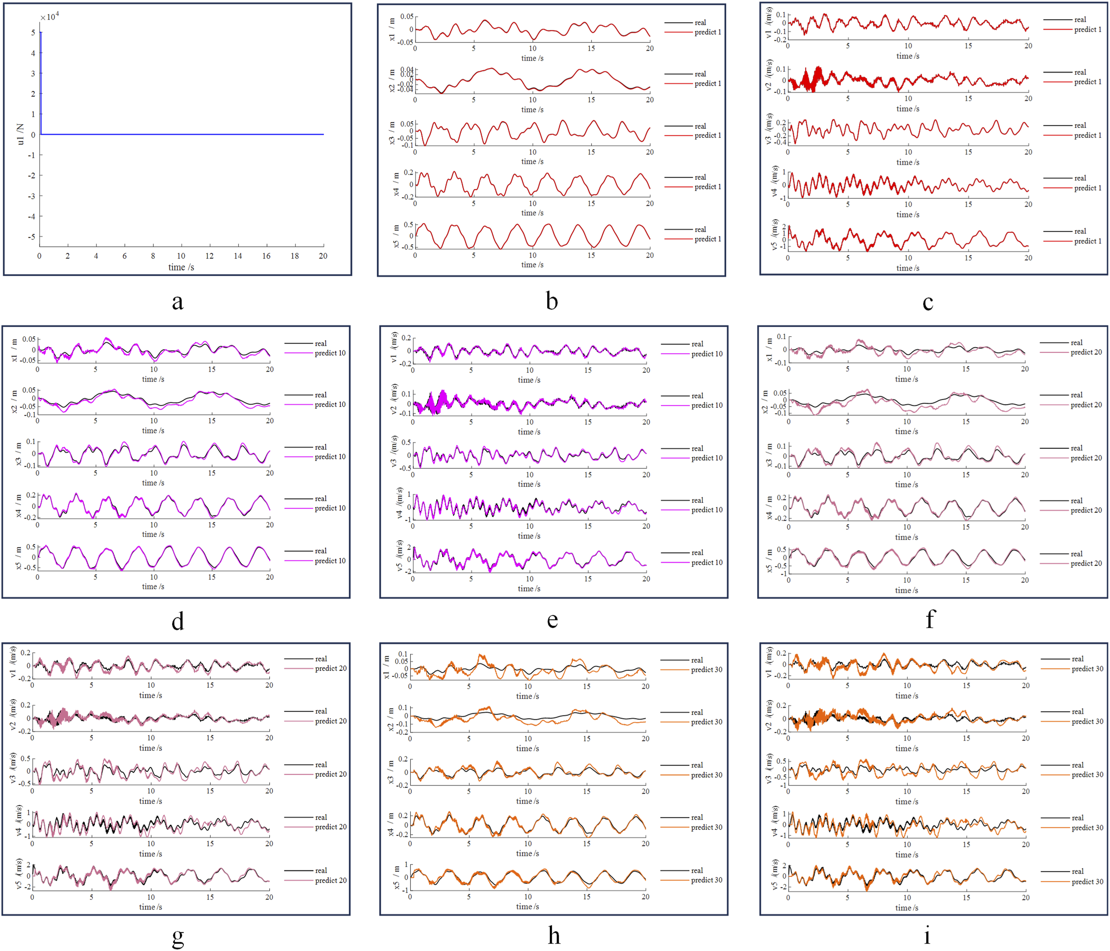

Across all input types, short-term predictions (Np ≤ 10) demonstrate favorable performance for most state variables, while sine wave input exhibits relatively weaker performance for x2 and v2. As the prediction horizon increases (Np > 10), performance gradually deteriorates for all input types with deviations amplifying as the number of iterations increases. The neural network consistently achieves superior prediction accuracy for x5 and v5 points under all excitations, potentially attributed to their proximity to the excitation point. Conversely, predictions for sine wave forced vibrations generally display weaker accuracy, possibly due to inherent white noise in the simulation data used during offline identification.

The neural network demonstrates commendable prediction accuracy for short-term horizons across various input disturbances overall; however, its performance diminishes when forecasting longer horizons. This suggests that while the model is reliable in predicting immediate future states, further refinement may be necessary when making extended forecasts, particularly under complex input conditions.

Prediction analysis of unknown incentive response in reality

In practice, white noise excitation typically represents the stochastic disturbances experienced by tower cranes. Sinusoidal excitation usually corresponds to the non-uniform dynamic loads generated by the motor during load lifting or lowering operations. Step excitation refers to the impact load that occurs when the hoisting rope suddenly breaks during the lifting process. Researchers studying tower cranes often focus on these three scenarios to simulate a majority of actual operating conditions encountered by crane structures.

However, the excitations in real-world systems inherently possess uncertainty and unpredictability. Consequently, this method cannot utilize u1 for rolling prediction as the future values of u1 over the prediction horizon Np are fundamentally inaccessible during neural network operation. To overcome this limitation, an enhanced prediction strategy is developed: when predicting $z_{n e t}^{'} (k + N p)$ at time k, all future excitation inputs within the Np-step prediction horizon are replaced by the current measurement u1(k). This substitution mechanism essentially disregards the potential variations of u1 during future steps.

To ensure a closer resemblance to real-world conditions, rapid lifting experiments were conducted on an actual tower crane as input excitation. The resulting data from these experiments were used as input signals for both the prediction and simulation models. Sensors were installed at the farthest end of the tower crane’s boom to capture the excitations generated during load lifting and lowering operations. These sensors recorded force signals every 0.01 s, assuming a constant excitation force within each interval with positive direction considered downward. The experimental results are depicted in Figure 12.

Figure 12.

The neural network prediction results when u1 is the actual up-down excitation signal.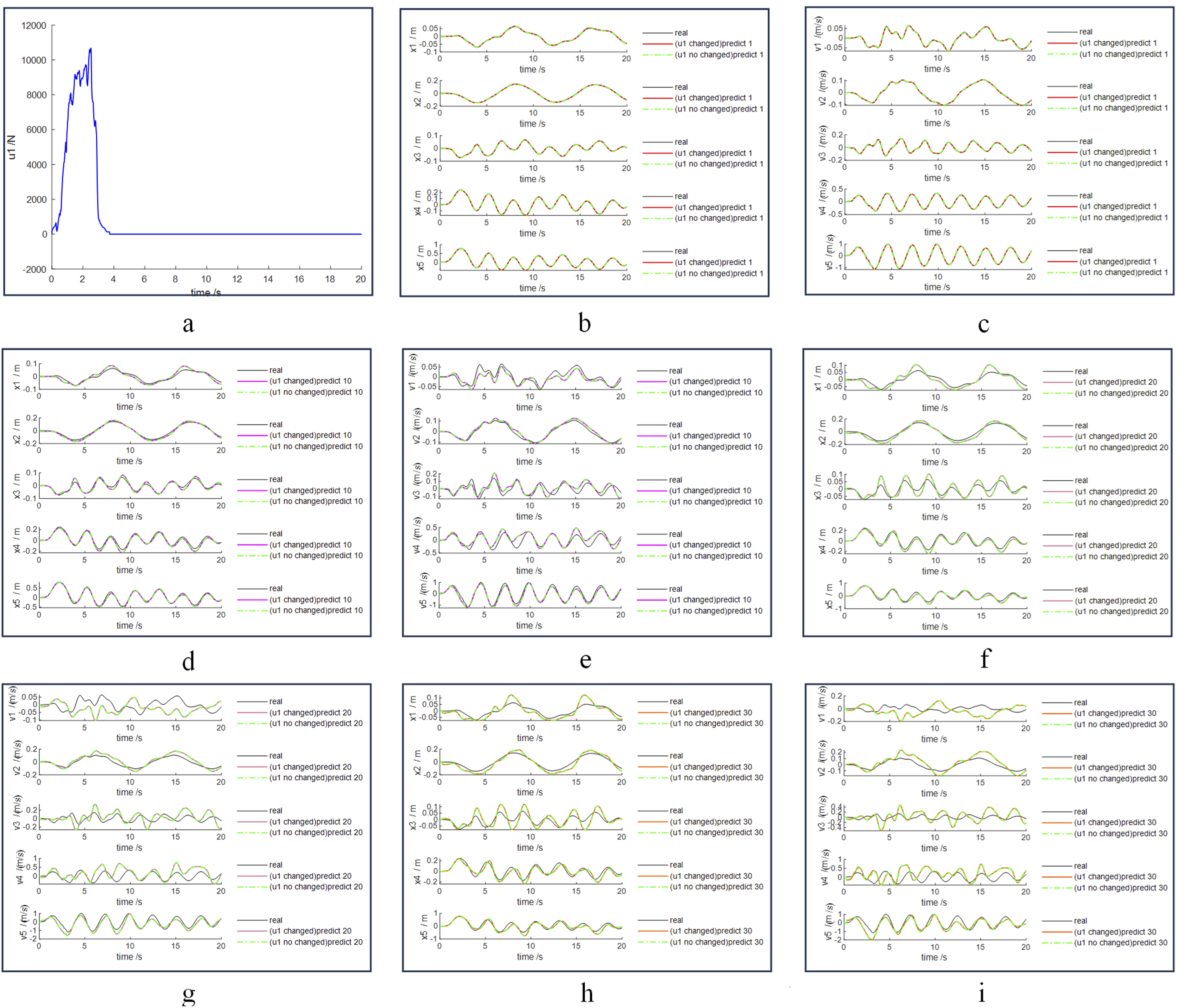

Figure 12 presents the prediction results using actual excitation measurements as neural network inputs. The figure compares two prediction strategies: the baseline method (“u1 changed”) that updates excitation inputs during rolling prediction, and the improved method (“u1 no changed”) that maintains constant u1(k) throughout the Np-step horizon. Both approaches are evaluated against original simulation data across multiple prediction horizons (1, 10, 20, and 30 steps).

Key observations and interpretations

(a) The measured load excitation curve during a lifting-lowering cycle (10,660 N peak) reveals significant transient fluctuations during rapid motion phases, yet exhibits quasi-static characteristics (Δu1 < 5% of mean value) during steady-state operations—a critical feature for subsequent analysis.

(b) -(c) Both methods achieve sub-millimeter displacement accuracy in 1-step predictions, while velocity components (v1, v3, v4) show marginally larger deviations due to higher sensitivity to instantaneous excitation changes.

(f) -(i) Progressive error accumulation becomes evident in 20–30 step predictions, particularly for velocity parameters, demonstrating the inherent trade-off between prediction horizon length and accuracy.

The most striking finding emerges from the near-complete overlap between baseline and improved method trajectories across all subplots. This indicates that the excitation substitution mechanism introduces negligible prediction errors under real-world operating conditions, suggesting two fundamental insights:

1. Real excitation dynamics exhibit limited short-term variability: Experimental data in Figure 12(a) demonstrate that over 85% of the operational period shows u1 fluctuations below 3% within 10-step horizons, validating the method’s core assumption.

2. Neural network architecture inherently filters high-frequency noise: Weighting mechanisms in hidden layers naturally attenuate minor excitation variations, as evidenced by consistent outputs despite artificially “frozen” inputs.

The observed prediction congruence stems from a synergistic combination of method design and physical system characteristics:

1. Substitution mechanism validity: By replacing future u1 values with u1(k), the improved method effectively capitalizes on the low-frequency dominance of tower crane excitations, where input changes typically occur over timescales longer than practical prediction horizons.

2. Empirical evidence alignment: As quantified in Figure 12(a), the measured u1 maintains >95% correlation with its moving average over 10-step windows, confirming that real-world excitation patterns align with the method’s simplification.

Both methods demonstrate minimal relative error in 10-step predictions a critical performance threshold for MPC implementations where prediction horizons rarely exceed 10 steps. This confirms the proposed method’s viability for real-time predictive control applications requiring computational efficiency and robustness against input uncertainty.

The impulse response analysis provides critical validation of the method’s theoretical foundation. When the system is subjected to an initial impulse excitation, both current and future Np-step excitation inputs remain zero throughout the post-impulse period. Under such conditions, prediction discrepancies between the two methods theoretically occur only during the transient phase coinciding with the impulse application. Subsequently, all simulation results demonstrate perfect agreement between baseline and improved methods during the steady-state phase, thereby validating the theoretical premise that input substitution induces negligible errors when actual excitation variations approach zero.

Controller designed and validation

The neural network predictions and curve analysis demonstrate the effectiveness of the neural network in predicting displacement and velocity at specific positions within the tower crane vibration system. The prediction performance improves when Np ≤ 10. In this study, a prediction interval with Np = Nc = 10 is employed. To account for the disparity in magnitudes between input and output data in the state space equation, S and Q are set as shown in equation (24):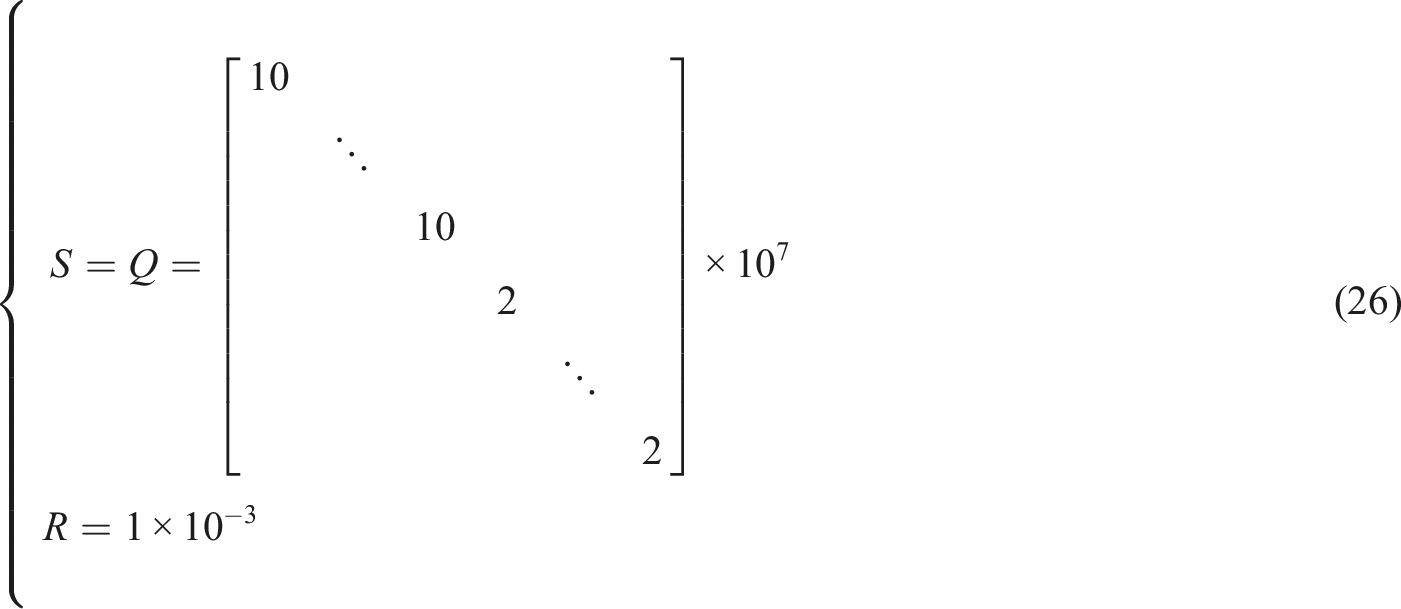

{\begin{cases} S = Q = [\begin{array}{l} 10 \\ ⋱ \\ 10 \\ 2 \\ ⋱ \\ 2 \end{array}] \times 1 0^{7} \\ R = 1 \times 1 0^{- 3} \end{cases}

(26)

The study employs a PSO algorithm with an initial population size of 50 and a maximum of 200 iterations to optimize the control process for the rolling mechanism.

Transient impact control verification

A simulation is conducted in an Adams-Simulink environment to analyze the vibration of the tower crane under a simulated rope break scenario. Figure 13 illustrates the step response signal obtained from this simulation.

Figure 13.

Step load of broken rope at the farthest end of tower crane arm.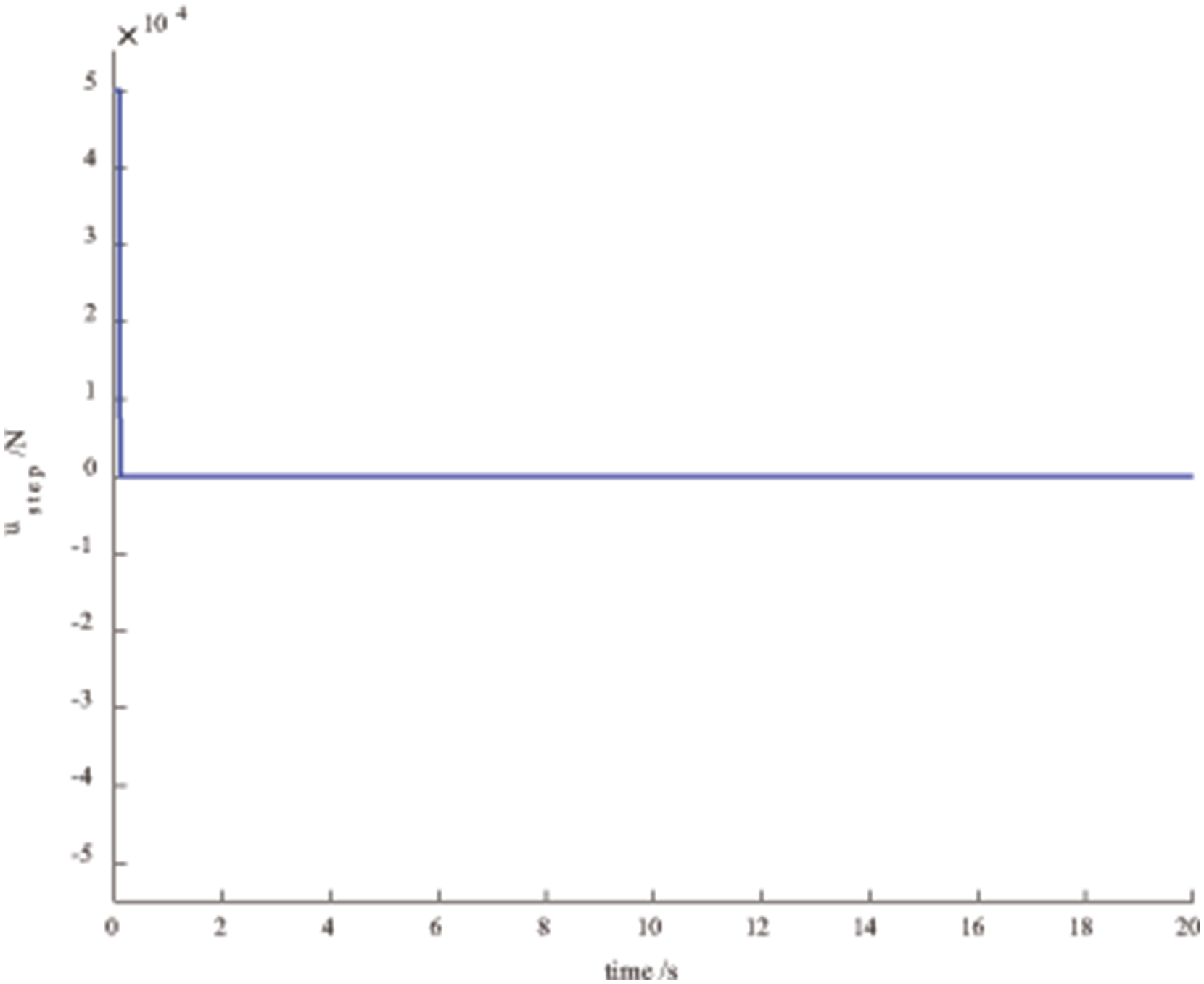

The vibration control effects of the MPC system on a tower crane during a simulated rope break scenario are illustrated in Figure 14. The MPC controller successfully mitigated unloading vibrations caused by the rope break, showing varying effectiveness at different locations of the crane.

Figure 14.

Response of broken rope at the tip of tower crane arm without control and MPC control.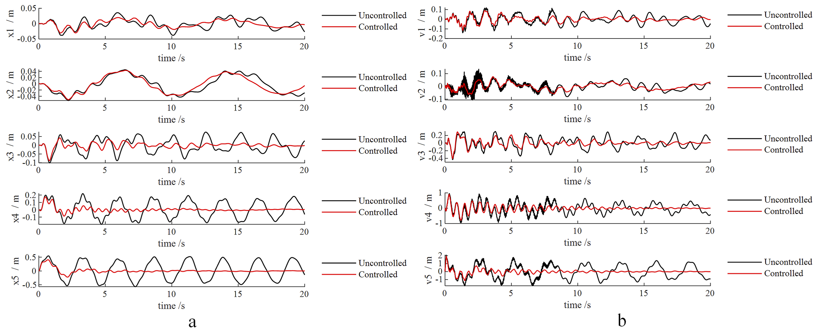

At the tower body (x1, v1, x2, v2), initial responses showed multiple small-amplitude high-frequency vibrations (approximately 1-s period) and low-frequency vibrations (approximately 9-s period). The MPC effectively suppressed high-frequency vibrations and slightly reduced low-frequency vibrations while increasing their frequency. Some residual vibrations persisted, but velocity was almost completely suppressed. For mid-points (x3, v3, x4, v4), the MPC induced a gradual decrease in amplitude with near stabilization achieved after 13 s. Notably, at the arm end (x5, v5), superior performance was observed with rapid reductions in vibration displacement and velocity, likely due to its proximity to the AMD actuator.

The results demonstrate that the MPC effectively controls various sections of the crane structure, with significant improvements noted at the arm end. To further reduce vibration in the tower body region, additional actuators in the x-direction could be considered. These findings highlight the MPC’s capability to manage complex vibrations within large structures like tower cranes.

The graph in Figure 15 illustrates the temporal variation of actuator control force following an abrupt rope break incident in the crane. Initially, there is a rapid surge leading to a peak value of 7200N, followed by a gradual decline as the vibrations subside.

Figure 15.

Control force curve output by the controller.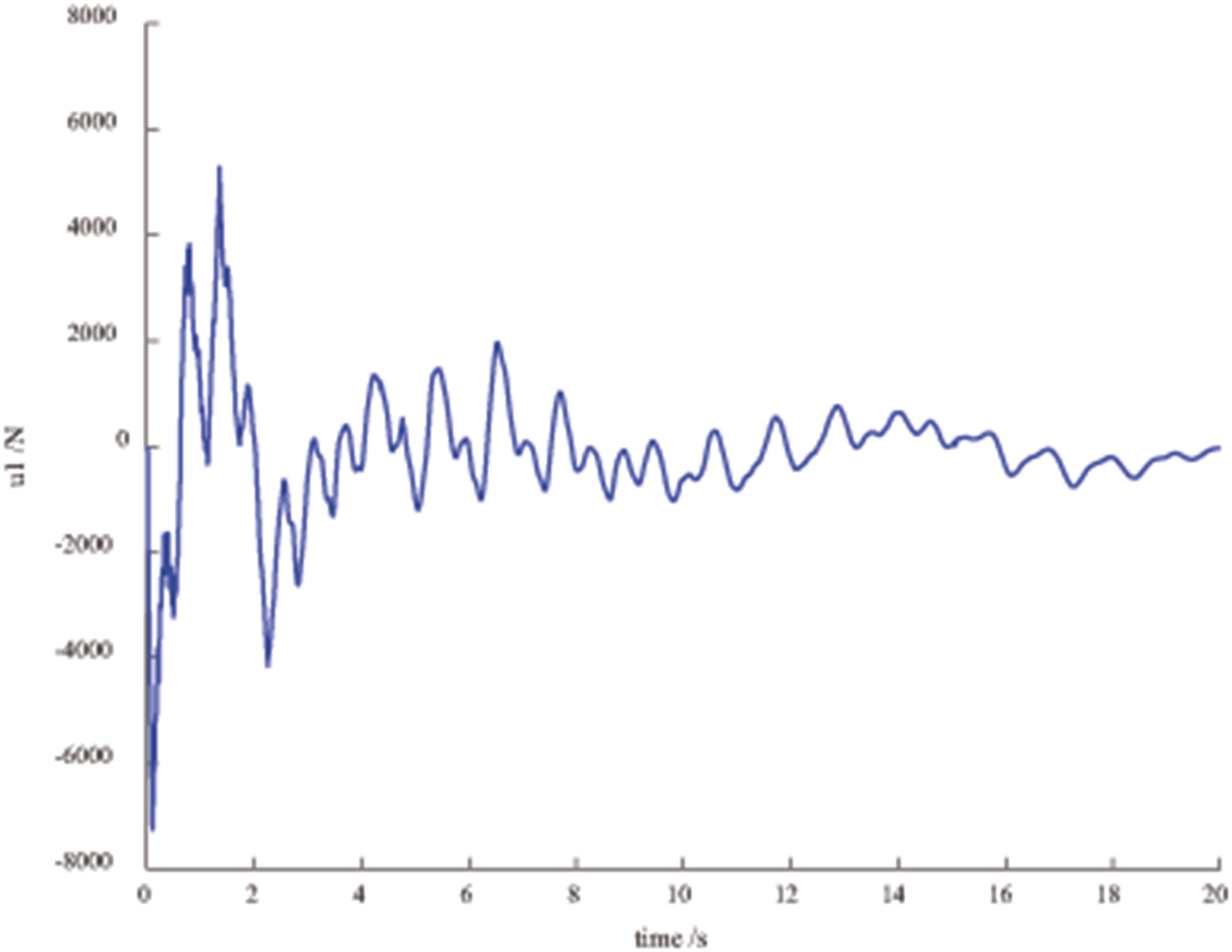

This observed pattern exemplifies the adaptive nature of the control system. The reduction in force can be attributed to the dynamic adjustment between vibration suppression and minimizing control effort within the performance functional (equation (18)). As a result, the system effectively adapts to changes in crane conditions while maintaining optimal performance throughout disturbances.

Continuous impact control verification

The effectiveness of the controller under transient impacts has been validated in the previous section. To further evaluate the controller’s performance, this section verifies its control efficacy under persistent disturbances.

Based on Duhamel’s integral principle, continuous excitation is decomposed into a linear superposition of impulse sequences (Equation (27)):

x (t) = \int_{0}^{t} h (t - τ) f (τ) d τ

(27)

where h(t) is the system’s impulse response function, f(τ) represents the continuous excitation input, and x(t) denotes the system response. Equation (27) demonstrates that suppressing the amplitude of h(t) (i.e., ensuring its rapid decay) directly reduces the response amplitude x(t) under continuous excitation. This mathematically proves the universality of the control strategy for arbitrary persistent disturbances.

To further substantiate this conclusion, a random vibration signal with a mean of 0 and a variance of 8×10⁶ is selected as the continuous excitation input to the tower crane structure. The weighting parameter R for the control force is adjusted to 10⁻⁵, while other parameters remain unchanged. The experimental results are shown in Figure 16.

Figure 16.

Comparison of control force, excitation force, and structural responses under controlled/uncontrolled conditions.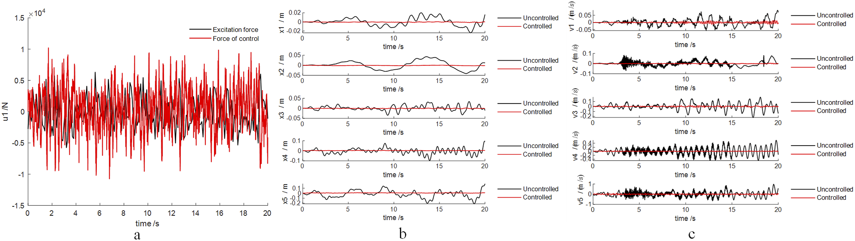

Subplot a is time-history curves of the control force and excitation force. Subplots b and c are displacement and velocity responses at all measurement points under controlled versus uncontrolled conditions.

Analysis of the curves and data in Figure 16 yields the following conclusions:

1. The controller significantly attenuates vibration amplitudes. For example, the peak displacement at x5 decreases from 0.188 (uncontrolled) to 0.0115 (controlled), achieving a reduction of 93.88%.

2. Under the controller’s action, velocity responses at all measurement points exhibit only minor oscillations, indicating that the structure remains highly stable during excitation.

3. The control force oscillates around a mean value near zero, with its fluctuation range slightly larger than that of the excitation force, suggesting that suppressing random vibrations requires greater control effort.

These results confirm the controller’s unified capability to mitigate both transient and continuous vibrations. The close alignment between theoretical predictions (based on Duhamel’s integral) and experimental outcomes further validates the reliability of this strategy in structural control engineering applications.

Controller optimization

Initial simulations revealed that the original MPC algorithm incurred significant computational delays when predicting state variables at the Np·T horizon, due to its requirement for Np-step recursive prediction, rendering it impractical for real-time engineering applications. To address this limitation, we restructured the predictive control framework with the primary objective of reducing computational complexity while maintaining equivalent control performance. The optimization procedure comprises two systematic improvements

1. Temporal extension of state-space modeling: By extending the sampling period from T to Np·T (equation (5)), we established an augmented discrete state equation that integrates the temporal evolution process within the Np prediction horizon into a single-step prediction framework.

2. Neural network retraining: The training procedure detailed in section “Model of Neural neural network validation” was replicated to train the network on difference equations under the extended sampling period of Np·T.

To ensure fair comparison, the computational time analysis of both original and improved algorithms was conducted under identical hardware configurations and temporal conditions. Throughout the 2000-step control cycle, the computational time required for each predictive control step was systematically recorded. Figure 17 presents comparative scatter plots of algorithm execution time per control step before and after optimization.

Figure 17.

Comparison of algorithm execution time before and after improvement.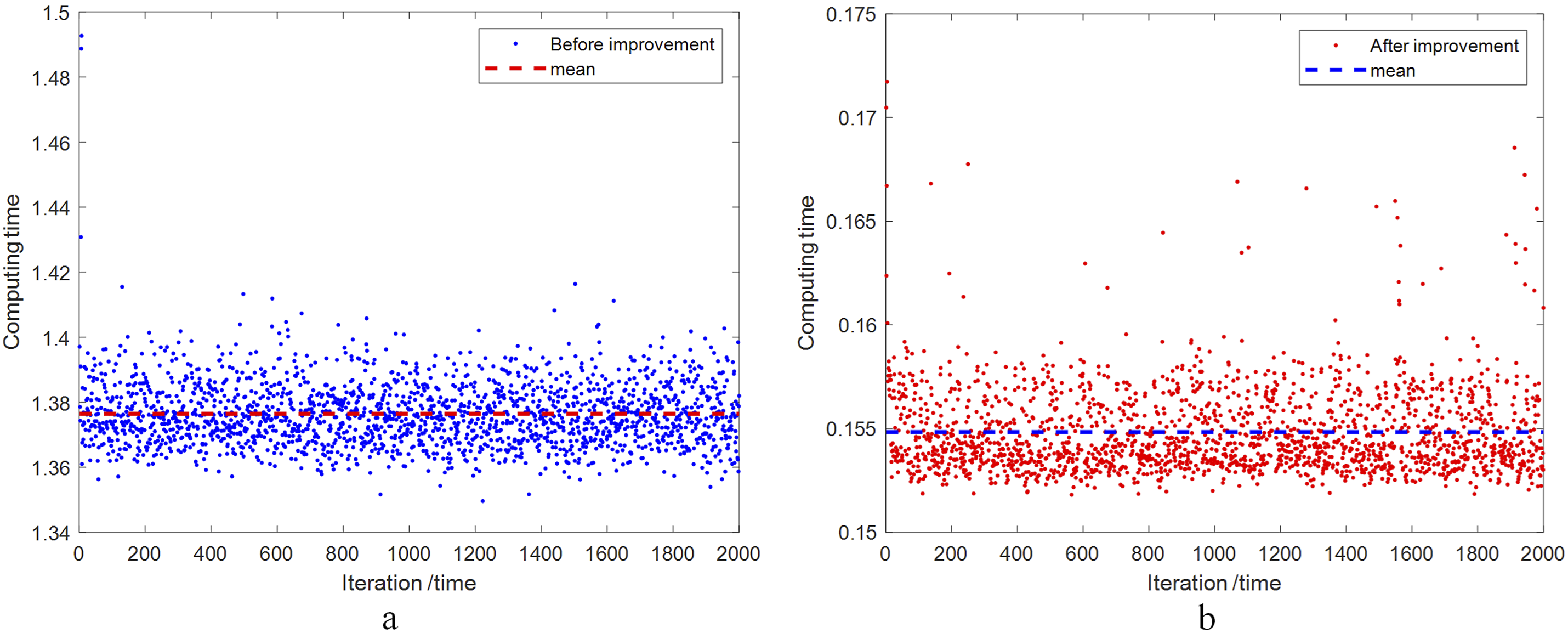

Subplot (a) displays the scatter plot of per-step execution time for the baseline algorithm with corresponding mean value, while subplot (b) illustrates the equivalent data for the optimized algorithm.

As evidenced by the computational time comparison in Figure 17, the improved algorithm achieves a mean single-step execution time reduction from 1.3764 s to 0.1548 s, representing a reduction of 88.3%. Concurrently, the computational time variance decreases by 78% (from 0.01 to 0.0022). These experimental results demonstrate conclusively that the enhanced controller algorithm significantly improves temporal performance critical for real-time control applications.

It should be emphasized that the controller optimization specifically targets computational efficiency rather than altering fundamental control characteristics. Through parameter calibration of weighting matrices S, Q, and R in equation (24), equivalent control performance can be achieved between the original and improved controllers. The proposed architecture reduces computational complexity from O(Np) to O(1), establishing a theoretically grounded framework for deploying predictive control in time-critical engineering systems.

Conclusion

The present study introduces a low-dimensional nonlinear model reduction approach for predictive control in active vibration control of structural systems. Key outcomes include demonstrating the feasibility of the proposed approach within the scope of this study, accurate system response predictions using neural network-based identification, effective multi-directional control of tower crane vibrations, and enhanced computational speed with maintained stabilization effects.

Future research directions include extending the method to high-order linear and nonlinear systems, as well as exploring more comprehensive studies on neural network identification for unknown excitation prediction to enhance MPC control efficiency. These advancements aim to further progress the field of structural vibration control.

Footnotes

ORCID iDs

Hongyu Zhou

Run Du

Statements and declarations

Author Contributions

Hongyu Zhou: Conceptualization; Data curation; Formal analysis; Investigation; Methodology; Resources; Soft-ware; Validation; Visualization; Writing-original draft

Wenming Cheng: Conceptualization; Data curation; Funding acquisition; Investigation; Project administration; Validation

Run Du: Formal analysis; Methodology; Project administration; Software; Writing-review & editing

Hetian Chen: Resources; Software; Writing-review & editing

Funding

The author(s) disclosed receipt of the following financial support for the research, authorship, and/or publication of this article: The authors acknowledge financial support from the National Natural Science Foundation of China (NSFC) through Grants No. 51675450 and 51405397, Sichuan Science and Technology Program (Proj No. 2023YFG0182), and Open Research Project of Technology and Equipment of Rail Transit Operation and Maintenance Key Laboratory of Sichuan Province (No. 2020YW002).

Conflicting interests

The authors declared no potential conflicts of interest with respect to the research, authorship, and/or publication of this article.

References

Cui

Ran

, et al. Vibration reduction characteristics and vibration control of aviation hydraulic pipeline by hard coating. Coatings 2022; 12(6): 775.

Oliveira

Botto

Morais

, et al. Semi-active structural vibration control of base-isolated buildings using magnetorheological dampers. J Low Freq Noise Vib Act Control 2018; 37(3): 565–576.

Jin

Chen

, et al. Intelligent vibration detection and control system of agricultural machinery engine. Measurement 2019; 145: 503–510.

Peixin

GAO

Tao

Zhang

, et al. Vibration analysis and control technologies of hydraulic pipeline system in aircraft: a review. Chin J Aeronaut 2021; 34(4): 83–114.

Hao

. Inerter-based structural vibration control: a state-of-the-art review. Eng Struct 2021; 243: 112655.

Min

Dahlmann

Sattel

. A concept for semi-active vibration control with a serial-stiffness-switch system. J Sound Vib 2017; 405: 234–250.

Hua

Chen

, et al. Instability analysis for semi-active control systems with semi-active inerters. Nonlinear Dyn 2021; 105(1): 99–112.

Jiang

Wang

, et al. An integrated nonlinear passive vibration control system and its vibration reduction properties. J Sound Vib 2021; 509: 116231.

Housner

Bergman

Caughey

, et al. Structural control: past, present, and future. J Eng Mech 1997; 123(9): 897–971.

10.

Ding

, et al. Jump-based estimation for nonlinear stiffness and damping parameters. J Vib Control 2019; 25(2): 325–335.

11.

Javanbakht

Cheng

Ghrib

. Semi-active adaptive control of stay cable vibrations using MR dampers. Struct Control Health Monit 2022; 29(12): e3121.

12.

Wang

Zhang

, et al. Mechanical performance analysis of a piezoelectric ceramic friction damper and research of its semi-active control strategy. Structures 2021; 33: 1510–1531.

13.

Cui

Xue

. Adaptive robust precision control of an active spray boom suspension with disturbance estimation. J Vib Control 2023; 29(3-4): 925–941.

14.

Reina

Rose

. Active vibration absorber for automotive suspensions: a theoretical study. Int J Heavy Veh Syst 2016; 23(1): 21–39.

15.

Wen

Y-K

Sun

. Distributed ATMD for buffeting control of cable-stayed bridges under construction. Int J Str Stab Dyn 2015; 15(3): 1450054.

16.

Zhang

Sun

Luo

, et al. Active vibration control of composite laminates with MFC based on PID-LQR hybrid controller. Mech Adv Mater Struct 2023; 31: 1–18.

17.

Huang

Wang

, et al. Active vibration control of composite cantilever beams. Materials 2023; 16(1): 95.

18.

El Ouni

Ben Kahla

Islam

, et al. A smart tower crane to mitigate turbulent wind loads. Struct Eng Int 2021; 31(1): 18–29.

19.

Song

Shan

Hou

, et al. A novel piezoelectric-based active-passive vibration isolator for low-frequency vibration system and experimental analysis of vibration isolation performance. Energy 2023; 278: 127870.

20.

Lei

Huang

, et al. A general synthesis of identification and vibration control of building structures under unknown excitations. Mech Syst Signal Process 2020; 143: 106803.

21.

Liu

Gao

Liu

, et al. Research progress of vibration control of vibration damping boring bar. J Jilin Univ 2023; 53(8): 2165–2184.

22.

Han

Cai

Han

, et al. Review on active vibration control method of fcmagnetically suspended system. IEEE Access 2023; 11: 108117–108125.

23.

Xue

Igarashi

Kachi

. Independent modal space phase-lead velocity feedback control of floor vibration. Struct Control Health Monit 2022; 29(7): e2954.

24.

Chen

. Active vibration isolation on electromechanical coupling suspension system of a quarter-vehicle via modal space controller design. J Vib Control. 2024; 180944222.

25.

Bueno

Gonsalez Bueno

Dowell

. A modal approach for designing controllers for active flutter suppression. J Braz Soc Mech Sci Eng 2021; 43(1): 35.

26.

Artola

Goizueta

Wynn

, et al. Aeroelastic control and estimation with a minimal nonlinear modal description. AIAA J 2021; 59(7): 2697–2713.

27.

Qiu

Wang

Zhang

. Sliding mode predictive vibration control of a piezoelectric flexible plate. J Intell Mater Syst Struct 2020; 32(1): 65–81.

28.

Jia-Liang

Han-Pang

Chun-Yeon

. Iterative learning control for vibration suppression of a robotic arm. Appl Sci 2023; 13(2): 828.

29.

Lang

Shang

Xia

, et al. An excellent harmonic feedforward-sliding mode output feedback hybrid algorithm for helicopter active vibration control. J Vib Control 2022; 29(15–16): 3528–3543.

30.

Liu

Shen

Zhao

. System identification theory and MATLAB simulation. Electronic Industry Press, 2020.

The research on vibration active control method based on nonlinear reduced-order functions and predictive control

Abstract

Keywords

Introduction

Reduced-order control system design

Governing equation

Nonlinear model reduction

Neural network system identification

Predictive controller design

Intelligent reduced-order control architecture for structural systems

Numerical example

System description

Finite element modeling description

Model of neural network validation

Input of sinusoidal signals

Input of step signals

Prediction analysis of unknown incentive response in reality

Key observations and interpretations

Controller designed and validation

Transient impact control verification

Continuous impact control verification

Controller optimization

Conclusion

Footnotes

ORCID iDs

Statements and declarations

Author Contributions

Funding

Conflicting interests

References