Sage Journals: Discover world-class research

Abstract

Objective: Blood pressure (BP) is a vital factor for human health and survival, and its elevation and fluctuations can have dangerous consequences on an individual’s well-being. Traditional BP measurement methods—including cuff-based devices and invasive arterial catheters—are unsuitable for continuous monitoring in daily life: cuffs are intermittent and uncomfortable, whereas arterial lines provide continuous data but are invasive and confined to clinical settings (e.g., ICUs/ORs). In response to this requirement, we propose a cuff-less, continuous, and noninvasive system for BP measurement using photoplethysmograph (PPG) signals and machine learning (ML) algorithms. Methods: In this investigation, we analyzed PPG signals acquired from a diverse cohort, with participants ranging in age from 21 to 86 years and including both healthy subjects and those with health conditions. The data underwent rigorous preprocessing and feature extraction procedures. To address computational efficiency and mitigate overfitting, we applied five distinct feature selection methods to refine the feature set. Subsequently, each method’s selected features were independently trained and tested using five ML regression algorithms to estimate systolic blood pressure (SBP) and diastolic blood pressure (DBP). Results: Our findings reveal that the ensemble-based extra trees (ET) algorithm, coupled with the SelectFromModel feature selection approach, surpassed competing algorithms in estimative performance. The ET algorithm achieved notably low root mean squared errors (RMSEs) of 5.21 for SBP and 2.65 for DBP, demonstrating its exceptional capability in the estimation of BP. Conclusion: The proposed approach demonstrates strong potential for accurate, non-invasive BP estimation. These findings have important implications for the development of wearable and mobile health technologies that support continuous, real-time BP monitoring for the prevention and management of hypertension and cardiovascular diseases.

Keywords

blood pressure photoplethysmograph machine learning feature extraction feature selection regression

Introduction

In the current healthcare landscape, the importance of effective blood pressure (BP) management is increasingly critical, especially considering its direct link to major health concerns such as cardiovascular diseases (CVDs), stroke, kidney failure, and peripheral arterial disease.¹ High BP, commonly known as hypertension, is a silent yet widespread health concern.² This urgency is underscored by striking global statistics. According to the World Health Organization (WHO), hypertension—a key risk factor for these conditions—affects approximately 1.28 billion adults aged 30–79 years worldwide.³ Alarmingly, about 46% of adults with hypertension are unaware of their condition.³ This contributes to increasing CVDs mortality rates,² projected to rise from 246 to 264 per one million from 2015 to 2030,^4,5 These figures highlight the imperative need for consistent and effective BP monitoring and management strategies. Such strategies are essential, not only for individual health but also for alleviating the broader public health burden posed by hypertension and its associated diseases. Despite the imperative need for consistent and effective BP monitoring, the prevalent methods for measuring BP, ranging from invasive procedures to noninvasive cuff-based techniques, present considerable challenges for continuous monitoring.

The invasive methods, involving the insertion of a thin tube into a vein, pose significant risks such as infection, localized bleeding, vein blockage, and potential damage to vein walls.⁶ This procedure demands a specialized medical team, expensive equipment, and may cause discomfort for patients.⁶ On the other hand, noninvasive cuff-based methods for BP measurement, while more accessible, are not without drawbacks. These techniques typically involve arterial occlusion, rendering them impractical for continuous monitoring purposes. Furthermore, the pressure exerted by these cuff-based methods can cause discomfort for some individuals. To overcome these challenges and usher in a new era of continuous and noninvasive BP measurement, innovative approaches have emerged, including wearable devices, mobile health applications, ultrasound technology, and hybrid approaches.^7–9 Specifically, mobile health applications have gained significant attention for their potential to enable continuous monitoring of BP using smartphones and wearable devices. These applications can collect real-time data, analyze it using cloud-based systems, and provide immediate feedback to users, fostering better adherence to BP management strategies and promoting long-term health monitoring outside of clinical environments. One promising method that has gained significant attention in the scientific community involves signal processing techniques based on photoplethysmography (PPG).^10–22

Plethysmography encompasses different types, each employing specific transducers to measure blood volume changes, which may vary across devices.²³ These include air plethysmography, strain-gauge plethysmography, electrical impedance plethysmography, and optical plethysmography, among others. Optical plethysmograms, categorized as PPG signals, provide volumetric measurements.²³ PPG signals provide a wealth of cardiovascular information, including blood oxygen levels, heart rate, blood volume changes, arterial stiffness, and valuable data for BP estimation,^24,25 Given their intricate nature and susceptibility to artifacts, a meticulous analysis is imperative for ensuring precise interpretation.²³

Typically, obtaining PPG signals involves the use of uncomplicated optical sensors equipped with both a light emitting diode (LED) and a corresponding photodetector. There are two distinct modes for PPG devices: transmission mode and reflection mode.²³ In transmission mode, the photodetector and LED are positioned on opposite sides of the tissue, allowing light to pass through. On the other hand, reflection mode involves installing the LED and photodetector on the same side of the tissue, enabling signal recording from backscattered light.²⁶ In extracting PPG waveforms, red, green, and infrared light are frequently employed. While red and infrared light have the ability to penetrate tissues to a depth of approximately 2.5 mm, green light has a lower penetration capacity of less than 1 mm,^27,28 Specifically, red light falls within the 600–750 nm wavelength range, while infrared light occupies the 850–950 nm wavelength range.²³ As a result, infrared light is commonly employed for acquiring PPG signals in BP measurement.²⁴ PPG has demonstrated its efficacy as a highly viable alternative for BP measurement methods.²³

As detailed in,²⁹ Martinez et al. investigated the correlation of arterial blood pressure (ABP) and PPG signals in both temporal and spectral domains. Their findings revealed that PPG possesses informational features consistent with ABP, with a waveform closely resembling that of ABP, suggesting PPG as a viable alternative to ABP. For understanding of PPG waveforms and their clinical relevance, refer to Figure 1. This figure illustrates a typical PPG waveform, emphasizing its three critical components: the systolic peak (indicating maximum arterial pressure during the cardiac cycle), the dicrotic notch (a minor dip post-systolic peak signifying aortic valve closure), and the diastolic peak (representing the minimal arterial pressure during cardiac relaxation).³⁰ Notably, these key points correspond to those observed in invasive BP measurement methods. Therefore, this correlation between the PPG waveform components and the key indicators in invasive BP measurement underscores the potential of PPG as a clinically significant, non-invasive tool for accurate BP monitoring. This alignment not only validates the effectiveness of PPG in capturing essential BP data but also highlights its advantage in offering a more patient-friendly and less cumbersome alternative to traditional methods.

Figure 1.

Illustration of a typical PPG waveform highlighting the systolic peak, dicrotic notch, and diastolic peak.

Recent research has introduced various methodologies for estimating BP from PPG signals. As detailed in,³¹ some of these algorithms employ waveform analysis combined with PPG-derived biometrics for BP estimation. Their efficacy has been assessed across a diverse population, varying in age, height, and weight. Upon calibration, PPG demonstrates considerable potential for monitoring BP fluctuations, presenting notable health and economic benefits. As detailed in,³² a bio-inspired mathematical model is introduced that employs comprehensive mathematical analysis of PPG signals for the estimation of systolic blood pressure (SBP) and diastolic blood pressure (DBP). This model marks a significant advancement in the domain of non-invasive BP monitoring, illustrating the potential of integrating mathematical precision with biomedical applications. Its emphasis on a bio-inspired approach offers a novel perspective in understanding and interpreting cardiovascular dynamics, potentially leading to more accurate and patient-friendly BP monitoring techniques.

Machine learning (ML) algorithms can be instrumental in analyzing PPG signals for BP estimation. A critical aspect of applying these ML techniques is feature engineering. PPG signals offer a diverse range of extractable features, including temporal characteristics, frequency-domain attributes, and morphological aspects,^28,33,34 Extensive research has explored a broad spectrum of features in this context. For instance, the study referenced in³⁵ extracted a total of 46 distinct features, whereas another investigation³⁶ employed 35 features. Furthermore, a separate study³⁷ utilized a composite set of features, encompassing time-domain, frequency-domain, and morphological characteristics, to enhance the model’s predictive accuracy. BP estimation can also be effectively achieved through models based on electrocardiogram (ECG) and PPG signals. These models leverage the combined data from ECG and PPG to enhance the accuracy of BP measurements. In the domain of BP estimation utilizing models based on ECG and PPG, these models predominantly rely on key features like Pulse Arrival Time (PAT) and Pulse Transit Time (PTT).³⁸

PTT has been a focal point in studies,^39,40 for predicting SBP and DBP levels. Research in⁴¹ expanded the scope by incorporating a combination of PAT and heart rate for BP prediction. This approach demonstrated superior predictive capabilities for SBP and DBP compared to using PTT alone, indicating the potential of integrating multiple physiological parameters for more accurate estimations. Further advancing the field, the beat-to-beat optical BP measurement technique, as detailed in,⁴² represents a significant leap. This method was exclusively developed using PPG signals obtained from fingertips. It involved extracting key features such as amplitudes and cardiac phase components through fast Fourier transformation (FFT). These features were then employed in training an artificial neural network (ANN), highlighting the evolving complexity and precision of non-invasive BP monitoring techniques and their potential in continuous and real-time health monitoring scenarios.

In the realm of BP monitoring through non-invasive methods, ML algorithms have shown promising results. A study outlined in⁴³ particularly highlights the efficacy of the support vector machine (SVM) algorithm, which exhibited superior accuracy in BP estimation compared to both linear regression and ANN methods. This finding underscores the potential of advanced ML techniques in the precise analysis of BP data. Building on this understanding, Chowdhury et al.²⁸ conducted a comprehensive analysis of PPG signals. In their study, a variety of features extracted from these signals were used to train and evaluate different ML algorithms. Notably, the integration of Gaussian process regression (GPR) with the ReliefF feature selection method demonstrated remarkable effectiveness, outperforming other algorithms in the accurate estimation of both SBP and DBP. This progression in research highlights the continuous evolution and refinement of ML applications in non-invasive cardiovascular monitoring.

The burgeoning field of deep learning (DL)⁴⁴ has recently catalyzed significant advancements in various medical applications. Among these, the study by Su et al.⁴⁵ addresses a critical issue in current BP estimation models derived from PPG signals—the challenge of accuracy degradation due to frequent calibration needs. To tackle this, they introduced a deep recurrent neural network (RNN) model, incorporating long short-term memory (LSTM) algorithms, tailored for time-series analysis of BP data. This model utilized both PPG and ECG data as inputs, showcasing the integration of multiple physiological signals in enhancing model accuracy. Complementing this approach, Gotlibovych et al.⁴⁶ explored the potential of using raw PPG data in detecting arrhythmias, achieving considerable success. This accomplishment not only reinforces the utility of PPG data in cardiovascular monitoring but also suggests the feasibility of employing raw PPG signals directly as inputs for DL models. Further extending the application of DL in this realm, a study by Slapničar et al.⁴⁷ developed a novel spectro-temporal deep neural network. This network was unique in its approach, taking not only the PPG signal but also its first and second derivatives as inputs, thus providing a more comprehensive analysis of the signal’s properties. Collectively, these studies highlight the progressive integration of DL techniques in the analysis of PPG signals, opening new avenues for accurate, non-invasive cardiovascular monitoring.

One of the significant challenges in applying DL techniques is the extensive time and computational resources required for model training. To address this limitation and explore more efficient alternatives, we focused on ML regression algorithms that are less computationally demanding while still offering strong predictive performance. Specifically, we investigated and compared five ensemble and tree-based ML regressors—Decision Tree (DT), Random Forest (RF), Extra Trees (ET), Gradient Boosting (GB), and CatBoost (CB). Among these, ensemble methods like ET and RF help reduce overfitting and enhance generalization by aggregating multiple decision trees. This comparative approach enabled us to systematically evaluate the trade-offs between training efficiency and estimation accuracy across different models.

In our research, we aimed to overcome several limitations identified in previous studies, employing strategies that reinforce the strengths of our approach:

• Sole Utilization of PPG Signals: Diverging from some previous studies that incorporated both PPG and ECG data, our methodology exclusively relies on PPG signals. This focus not only simplifies the computational requirements but also enhances the efficiency and applicability of our approach in practical scenarios.

• Larger Sample Size: We expanded our research to include a more extensive number of subjects compared to some past studies, enhancing the robustness and generalizability of our findings.

• Employing ML Algorithms: Rather than relying on a single technique, our study systematically compares distinct ML algorithms. This comparative approach allows us to assess the trade-offs between computational efficiency and predictive accuracy, providing a more balanced perspective on model performance.

As a result of implementing these strategies, our study achieved improved outcomes in the separate estimation of SBP and DBP, reflecting the efficacy of our chosen methodologies and algorithm. Thus, our research demonstrates the potential of utilizing PPG signals and ML techniques for BP estimation. Furthermore, it successfully overcomes prior constraints observed in previous studies, such as limited sample sizes, reliance on both PPG and ECG signals, and the high training time associated with DL models, presenting a hopeful trajectory for practical implementation in cardiovascular monitoring and assessment.

The article is organized as follows: Section 2 offers an overview of the methodology, Section 3 discusses the results, Section 4 provides the discussion, and Section 5 provides the conclusion.

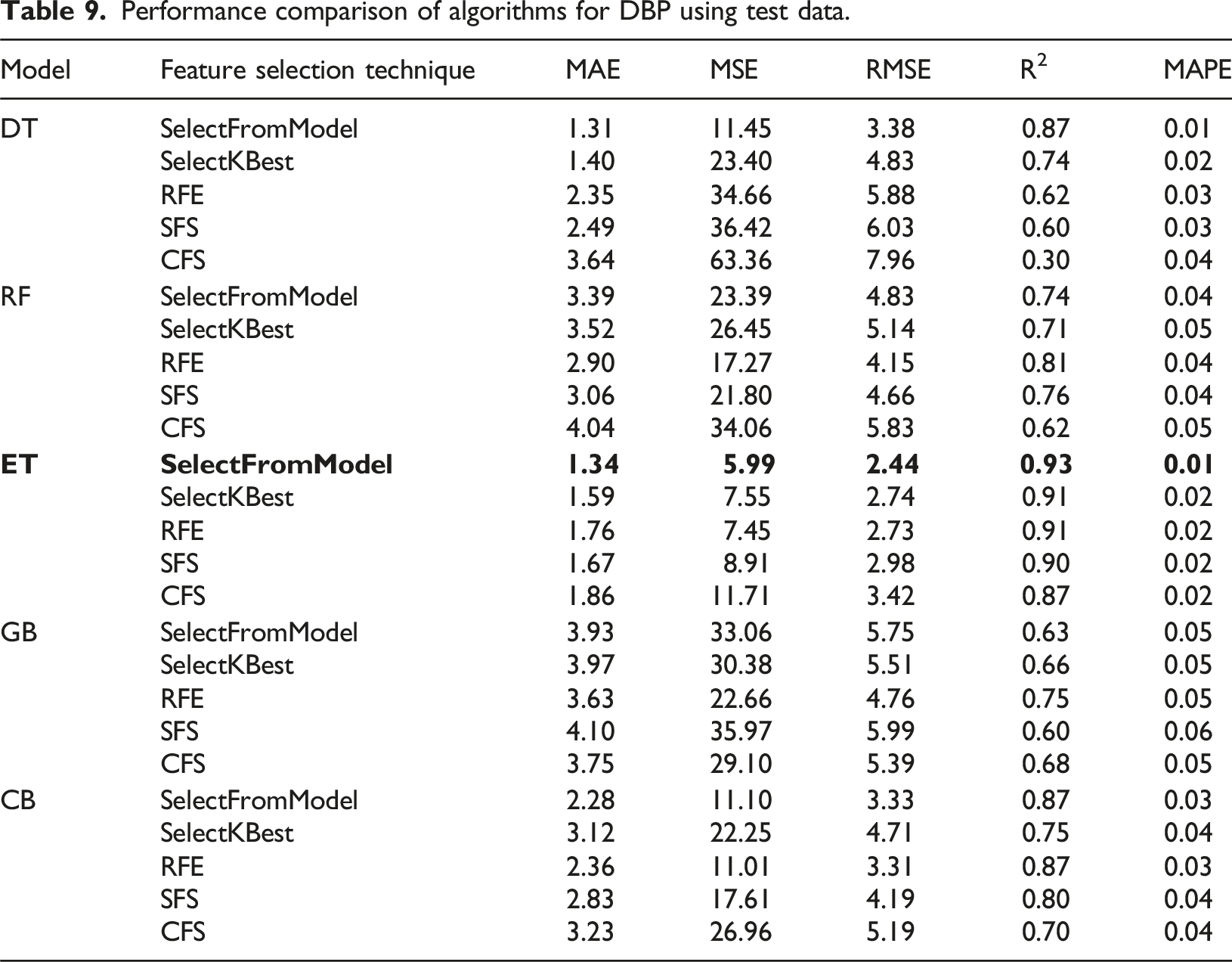
Material and methods

This section provides a comprehensive overview of the steps used to estimate BP, including the data used, signal preprocessing techniques, feature extraction methods, as well as feature selection techniques and the ML algorithms employed. Figure 2 illustrates the initial phase of our methodology, which entailed a rigorous assessment of PPG signals quality to confirm their reliability for further analysis. The PPG signals were then subjected to a series of preprocessing steps to prepare them for feature extraction. Subsequent to the extraction process, feature selection techniques were applied to both reduce computational complexity and minimize the risk of overfitting. The resulting dataset was shuffled and randomly divided into two subsets: 80% was dedicated to training the ML algorithms, and the remaining 20% was reserved for evaluating algorithmic performance. The training and evaluation of the ML algorithms were conducted using a 10-fold cross-validation approach to ensure robustness and generalizability of our model.

Figure 2.

Methodological flowchart: From PPG signals quality assessment to ML algorithms evaluation.

Database description and collection protocol

The dataset underpinning our investigation, procured from Liang et al.,²⁴ is a publicly accessible compendium of data from 219 adults, ranging in age from 21 to 86 years, with a near-equal gender distribution of 48% male and 52% female participants. These individuals were involved in experimental sessions lasting about 15 min each, during which they were first acclimatized to the environment for 10 min to ensure a stabilized physiological state. Comfortably seated and with minimal interference, participants then underwent the data collection phase. In this phase, raw PPG signals were directly recorded from the participants. Each subject had three separate non-overlapping PPG recordings, each lasting 2.1 s (2100 samples at a sampling rate of 1 kHz with 12-bit resolution).²⁴ Immediately after the three PPG acquisitions, blood pressure was measured using a sphygmomanometer by a trained nurse. The entire PPG acquisition and BP measurement process lasted approximately 3 min. The PPG signal was sourced from the left index finger’s tip, and BP measurement were meticulously taken from the right forearm. In total, the database therefore contains 657 raw PPG segments (3 segments × 219 participants). Of these, 282 high-quality segments were selected and used in the present study; additional details of the selection procedure are provided in later sections.

In addition to the rich demographic spectrum, the breadth of health statuses among the participants—ranging from healthy to various pathological conditions—was a decisive factor in selecting this database. This diversity is critical for our research on physiological variations, as it allows for a nuanced analysis of PPG signals across a broad spectrum of the population. Figure 3 exemplifies this by showcasing PPG waveforms from four distinct individuals of varying ages and health conditions, with Table 1 elaborating on the database specifics. Younger, healthy subjects with normal BP present PPG waveforms with all characteristic features, such as the dicrotic notch and diastolic peak, visibly intact. In contrast, PPG waveforms from older or ailing subjects exhibit discernible deviations, with these features becoming increasingly subdued or altered—a testament to the physiological impacts of aging and health deterioration.²³ Such variations underscore the necessity for advanced analytical techniques, which our study seeks to address.

Figure 3.

Illustrative PPG signal variability across different health profiles: This figure is pivotal in demonstrating the diversity of PPG signals across a spectrum of ages and health conditions, underscoring the relevance and necessity of our study. Panel (a) shows the PPG signal of a 25-year-old healthy woman with normal BP, serving as a baseline reference. Panel (b) presents the signal from a 59-year-old man with prehypertension and cerebrovascular disease, illustrating the alterations in the PPG signal due to cardiovascular changes. Panel (c) depicts the signal of a 63-year-old woman with stage 1 hypertension and type 2 diabetes, further highlighting the PPG signal’s sensitivity to varying health states. Lastly, panel (d) exhibits the signal from a 78-year-old man with stage 2 hypertension and a history of cerebral infarction, showcasing the pronounced signal differences in advanced cardiovascular conditions.

Table 1.

Demographic and health characteristics of the study population⁴⁸.

Physical parameter	Statistical information
Females	115 (52%)
Males	104 (48%)
Weight (kg)	60 ± 11
Height (cm)	161 ± 8
Age (years)	57 ± 15
Body Mass Index (BMI) (kg/m²)	23 ± 4
SBP (mm Hg)	127 ± 20
DBP (mm Hg)	71 ± 11
Heart rate (beats/min)	73 ± 10
Hypertension	57 (26%)
Diabetes	38 (17.3%)
Vascular Infarction	29 (13.2%)

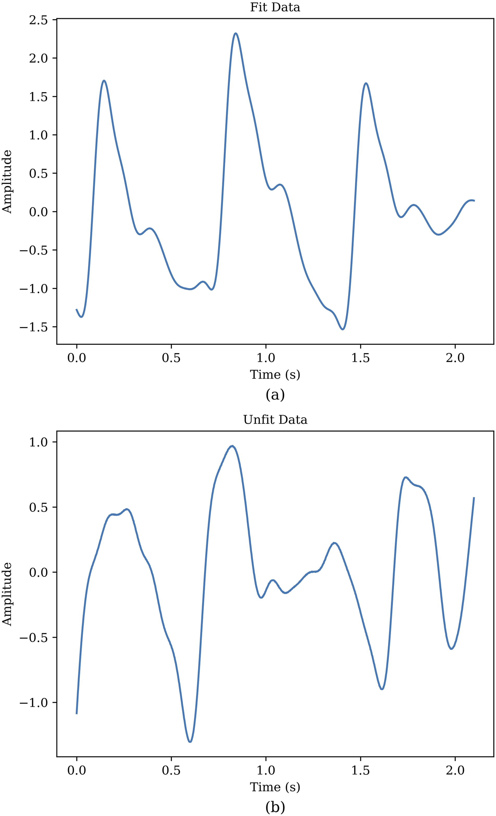
However, a challenge arose when assessing the quality of PPG signals in the dataset. Out of the total 657 signals, a considerable number exhibited low quality and were deemed unsuitable for feature extraction. To address this issue, Liang et al.⁴⁸ employed a signal quality index (SQI) based on skewness, the formula for which is presented in equation (1), to identify suitable signals. The results of their research are documented in a separate file accompanying the database. The application of this SQI, followed by a rigorous quality assurance process that filtered the data based on skewness, led to the retention of 282 signals for our analysis. Signals with aberrant or non-standard PPG waveforms, or those lacking distinct features necessary for accurate interpretation, were systematically excluded. It is worth noting that the retained subset covers the same age range and diversity of health conditions as the original dataset. This meticulous selection process, while reducing the number of usable signals, significantly enhanced the reliability and validity of the subsequent analyses, ensuring that only high-quality data were utilized in our study. Figure 4 provides a comparative visualization, delineating both the exemplar and the disqualified signals, thereby illustrating the stringent selection criteria employed to ensure the integrity of our study’s data pool.

S = \frac{1}{N} {\sum_{i = 1}^{N} (x_{i} - μ / σ)}^{3}

(1)

where:

• S represents the Skewness of the PPG signal.

• N is the number of samples in the PPG signal.

• x_i refers to the i-th sample value in the PPG signal.

• μ denotes the mean value of the PPG signal.

• σ signifies the standard deviation of the PPG signal.

Figure 4.

Comparative analysis of fit and unfit PPG waveforms. Panel (a) displays a fit waveform exhibiting clear diastolic and systolic peaks with distinct features. Panel (b) depicts an unfit waveform where the key features are less pronounced or absent, indicating lower signal quality.

Preprocessing of PPG signals

Before feature extraction, the raw PPG signals went through various preprocessing steps including normalization, filtering and baseline correction, which are as follows:

Normalization

In order to derive valuable insights from the signals, it was imperative to normalize the signal data. This study employed the Z-score technique for signal normalization, which involved transforming the signals into amplitude-limited data by centering them around their mean and scaling them by their standard deviation. This normalization process ensures that the signals have a consistent scale and facilitates meaningful comparisons and analysis across different data points. It was noticed that the implementation of other preprocessing techniques became more straightforward following the normalization process.

Z = \frac{x - μ}{σ}

(2)

where:

• Z is the normalized PPG signal value.

• x is the raw PPG signal value to be normalized.

• μ is the mean of the PPG signal values.

• σ is the standard deviation of the PPG signal values.

Filtering

In our analysis, we observed the presence of high-frequency and low-frequency noise components in the signals obtained from the database.²⁴ To address the occurrence of noise components, various filters were tested for filtering PPG signals^48–52 and removing unwanted noise (including moving average filter, Butterworth filter, wavelet de-noising filter, and Chebyshev filter⁴⁸). Ultimately, we applied a Chebyshev II filter to the signals, designed with a filter order of four and a cutoff frequency of 12 Hz. This was implemented in Python 3.9.13 using the SciPy library (v1.9.3). Figure 5 illustrates both the normalized raw signal and the filtered signal, highlighting the effectiveness of this filtering process.

Figure 5.

Comparison of normalized raw PPG signal with the filtered signal over time.

Baseline correction

The PPG waveform often exhibits baseline wandering as a result of respiratory activity, occurring within a frequency range of 0.15 to 0.5 Hz.^53–55 Consequently, it is crucial to effectively filter the signal to eliminate this baseline wandering while retaining essential information. To achieve this, we employed a polynomial fit to identify the signal’s underlying trend. Subsequently, we subtracted this trend from the signal to obtain the baseline-corrected signal,²⁸ as depicted in Figure 6. We experimented with polynomial degrees ranging from 3 to 6, and found that a degree of 5 provided the best result. This was implemented in Python 3.9.13 using the NumPy library (v1.23.5).

Figure 6.

Comparison of the filtered PPG signal with baseline wandering and the signal after detrending process.

Feature extraction

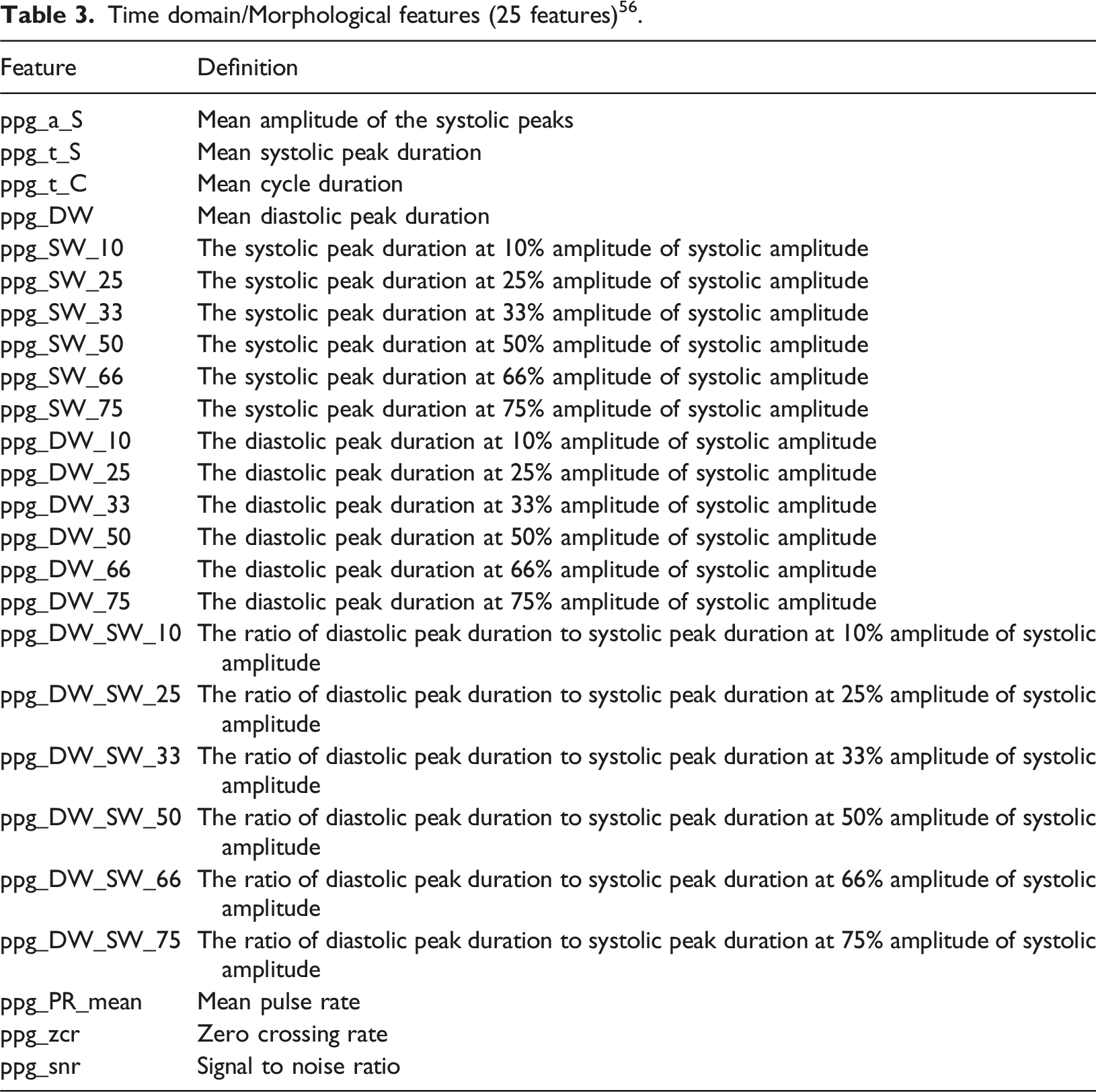
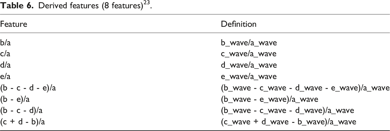
The feature extraction process was conducted in three distinct parts. Firstly, a comprehensive set of features was extracted using the BIOBSS⁵⁶ library in Python. BIOBSS, a Python package created on Feb 2, 2023, can be succinctly described as a biological signal processing and feature extraction library. Features extracted in this phase are reported in Tables 3–5, which focus on time-domain, morphological, frequency-domain, and statistical characteristics of the PPG signals.

Secondly, another set of features was derived using a series of specifically designed formulas²³ These formulas were carefully chosen to capture characteristics and nuances of the PPG signals, enhancing the depth of the feature extraction process. Features derived from these formulas are reported in Tables 2 and 6. Finally, we formed a separate set of features using participants demographic information collected at the beginning of the database registration process and reported with the database file. These demographic features, such as age, sex, BMI, and medical history, are reported in Table 7. A total of 71 features were extracted, which are reported in Tables 2–7.

Table 2.

Signal key points as feature set (12 features)²³.

Feature	Definition
O_wave	Systolic notch
S_wave	Systolic main peak
N_wave	Diastolic notch or dicrotic notch
D_wave	Dicrotic peak or diastolic peak
w_wave	The maximum slope peak in systolic of VPG waveform
y_wave	The global minima slope in systolic of VPG waveform
z_wave	The maximum slope peak in diastolic of VPG waveform
a_wave	Early systolic positive wave
b_wave	Early systolic negative wave
c_wave	Late systolic reincreasing wave
d_wave	Late systolic redecreasing wave
e_wave	Early diastolic positive wave

Table 3.

Time domain/Morphological features (25 features)⁵⁶.

Feature	Definition
ppg_a_S	Mean amplitude of the systolic peaks
ppg_t_S	Mean systolic peak duration
ppg_t_C	Mean cycle duration
ppg_DW	Mean diastolic peak duration
ppg_SW_10	The systolic peak duration at 10% amplitude of systolic amplitude
ppg_SW_25	The systolic peak duration at 25% amplitude of systolic amplitude
ppg_SW_33	The systolic peak duration at 33% amplitude of systolic amplitude
ppg_SW_50	The systolic peak duration at 50% amplitude of systolic amplitude
ppg_SW_66	The systolic peak duration at 66% amplitude of systolic amplitude
ppg_SW_75	The systolic peak duration at 75% amplitude of systolic amplitude
ppg_DW_10	The diastolic peak duration at 10% amplitude of systolic amplitude
ppg_DW_25	The diastolic peak duration at 25% amplitude of systolic amplitude
ppg_DW_33	The diastolic peak duration at 33% amplitude of systolic amplitude
ppg_DW_50	The diastolic peak duration at 50% amplitude of systolic amplitude
ppg_DW_66	The diastolic peak duration at 66% amplitude of systolic amplitude
ppg_DW_75	The diastolic peak duration at 75% amplitude of systolic amplitude
ppg_DW_SW_10	The ratio of diastolic peak duration to systolic peak duration at 10% amplitude of systolic amplitude
ppg_DW_SW_25	The ratio of diastolic peak duration to systolic peak duration at 25% amplitude of systolic amplitude
ppg_DW_SW_33	The ratio of diastolic peak duration to systolic peak duration at 33% amplitude of systolic amplitude
ppg_DW_SW_50	The ratio of diastolic peak duration to systolic peak duration at 50% amplitude of systolic amplitude
ppg_DW_SW_66	The ratio of diastolic peak duration to systolic peak duration at 66% amplitude of systolic amplitude
ppg_DW_SW_75	The ratio of diastolic peak duration to systolic peak duration at 75% amplitude of systolic amplitude
ppg_PR_mean	Mean pulse rate
ppg_zcr	Zero crossing rate
ppg_snr	Signal to noise ratio

Table 4.

Frequency domain features (8 features)⁵⁶.

Feature	Definition
ppg_pow	Power of the signal at a given range of frequencies
ppg_rpow	Ratio of the powers of the signal at given ranges of frequencies
ppg_p_1	The amplitude of the first peak from the FFT of the signal
ppg_f_1	The frequency at which the first peak from the FFT of the signal occurred
ppg_p_2	The amplitude of the second peak from the FFT of the signal
ppg_f_2	The frequency at which the second peak from the FFT of the signal occurred
ppg_p_3	The amplitude of the third peak from the FFT of the signal
ppg_f_3	The frequency at which the third peak from the FFT of the signal occurred

Table 5.

Statistical features (9 features)⁵⁶.

Feature	Definition
ppg_mean	Average value of the signal
ppg_median	Middle value of the signal
ppg_std	Standard deviation of the signal
ppg_pct_25	25th percentile of the signal
ppg_pct_75	75th percentile of the signal
ppg_mad	Mean absolute deviation of the signal
ppg_skewness	Skewness of the signal
ppg_kurtosis	Kurtosis of the signal
ppg_entropy	Entropy of the signal

Table 6.

Derived features (8 features)²³.

Feature	Definition
b/a	b_wave/a_wave
c/a	c_wave/a_wave
d/a	d_wave/a_wave
e/a	e_wave/a_wave
(b - c - d - e)/a	(b_wave - c_wave - d_wave - e_wave)/a_wave
(b - e)/a	(b_wave - e_wave)/a_wave
(b - c - d)/a	(b_wave - c_wave - d_wave)/a_wave
(c + d - b)/a	(c_wave + d_wave - b_wave)/a_wave

Table 7.

Demographic features (9 features).

Feature
Age
Sex
BMI
Height
Weight
Heart rate
Diabetes
Cerebral infarction
Cerebrovascular disease

Feature selection

In this study, we utilized five feature selection techniques: SelectFromModel,⁵⁷ SelectKBest,⁵⁷ Recursive Feature Elimination (RFE),⁵⁷ Sequential Feature Selection (SFS),⁵⁷ and Correlation-Based Feature Selection (CFS).⁵⁸ These techniques were implemented leveraging Python’s built-in functions. Their primary role was to identify the most relevant features for our analysis. Below, we provide a brief description of each of these feature selection techniques.

SelectFromModel

SelectFromModel is a feature selection technique commonly used in ML. It works by training a ML model (e.g., a DT or a linear model) and then selecting the most important features based on the model’s internal feature importance scores⁵⁷ This method allows you to choose features that contribute the most to the model’s estimation performance, thus reducing the dimensionality of the data while preserving relevant information.

SelectKBest

SelectKBest is a simple and straightforward feature selection technique. It evaluates each feature’s individual statistical significance with respect to the target variable using statistical tests like mutual information regression.⁵⁷ Then, it selects the top K features with the highest scores. This method is particularly useful when you want to specify a fixed number (K) of features to retain.

Recursive Feature Elimination

RFE is an iterative feature selection technique. It starts with all features and recursively removes the least important ones. The importance of features is determined by training a model and examining feature weights or coefficients. RFE continues to eliminate features until the desired number or a predetermined threshold is reached⁵⁷ This method is effective for selecting a subset of features while maintaining model performance.

Sequential Feature Selection

SFS is an iterative technique that systematically adds or removes features from the model. It works by selecting or excluding features one at a time based on their contribution to model performance. The process involves evaluating different feature subsets to identify the most informative combination. During each iteration, SFS considers the influence of each feature on the predictive power of the model. This method is valuable for finding the optimal subset of features that maximizes model accuracy while minimizing dimensionality.⁵⁷

Correlation-based Feature Selection

CFS functions as a feature selection technique, assessing the correlation between features and the target variable. It measures how well each feature is related to the outcome of interest. Additionally, CFS assesses the intercorrelations among features to avoid redundancy. Features that have high correlations with the target variable and low correlations with each other are selected, resulting in a subset of relevant and non-redundant features.⁵⁸

These feature selection techniques are crucial for improving the performance and interpretability of ML algorithms by identifying and retaining the most informative features while reducing the risk of overfitting, where models become too specialized to the training data and perform poorly on new, unseen data.

Machine learning algorithms

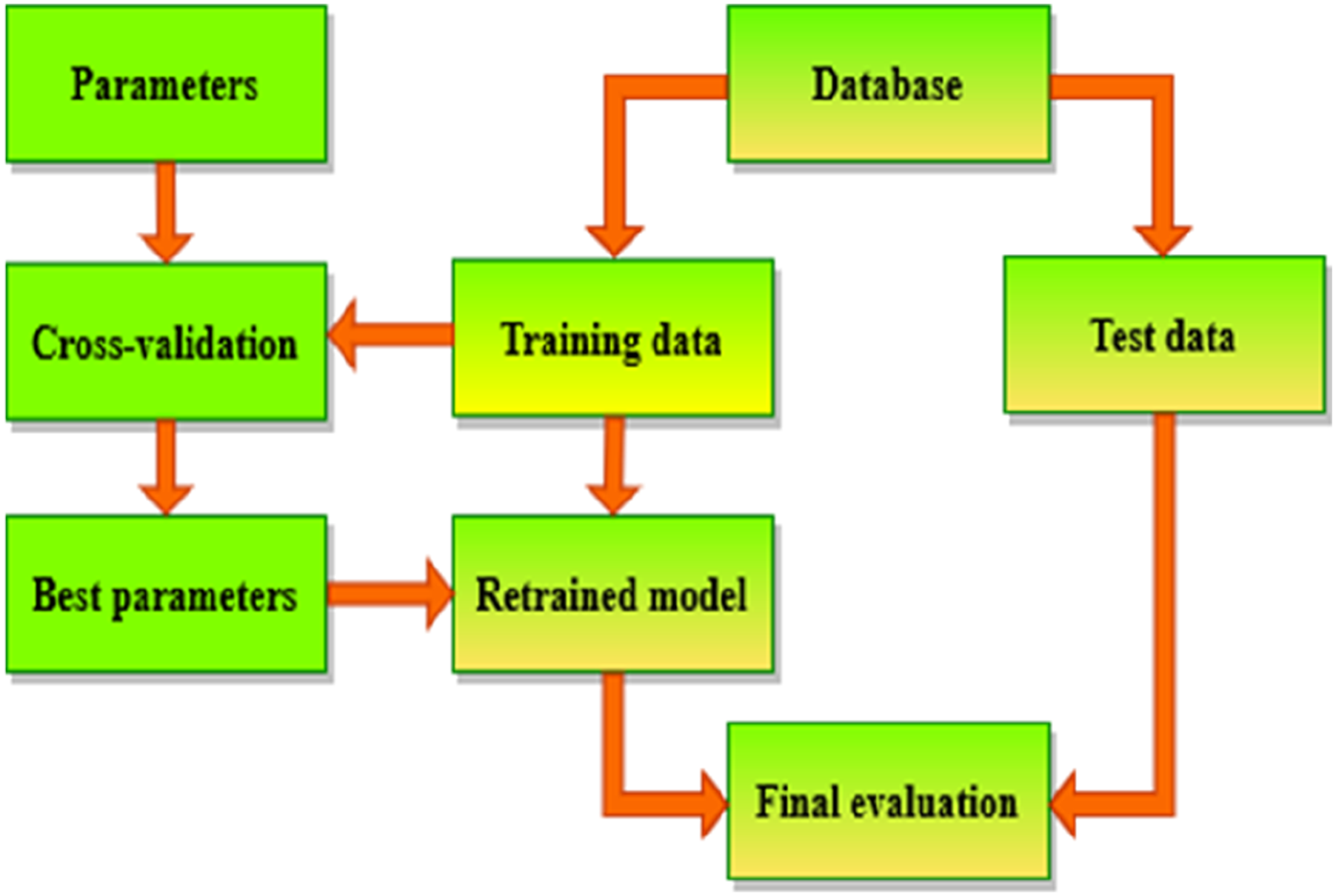
After extracting features and using feature selection methods, we trained and evaluated 10 different algorithms using 10-fold cross-validation, and in the following, we report the results of five of the best ones. The obtained data were shuffled and then randomly divided into two subsets: 80% for training, and 20% for evaluating algorithm performance. Here’s an explanation of the 10-fold cross-validation method,⁵⁹ and the whole process is shown in Figure 7:

(1) Train data Splitting:

-The train dataset is divided into 10 equal-sized folds.

(2) Training and Validation:

- The model is trained and evaluated 10 times, each time using a different fold as the validation set and the remaining 9 folds as the training set.

- In the first iteration, the first fold is used as the validation set, and the model is trained on the remaining 9 folds. In the second iteration, the second fold is used as the validation set, and so on.

(3) Performance Metrics:

- Performance metrics are recorded for each iteration.

(4) Average Performance:

- The performance metrics from all 10 iterations are averaged to obtain a more reliable estimate of the model’s performance.

(5) Parameter Tuning:

- If the model has hyperparameters that need to be tuned, this process is repeated for different combinations of hyperparameters.

(6) Best Parameters Selection:

- The hyperparameters that result in the best average performance across the 10 folds are selected.

(7) Final Model Training:

-The final model is trained on the entire dataset using the selected hyperparameters.

(8) Model Evaluation:

-The performance of the final model is evaluated on a test set that was not used during training or cross-validation.

Figure 7.

Flowchart of cross-validation workflow in model training.

We evaluated the performance of ML algorithms in BP estimation using five criteria,^28,60 In this context, ‘ŷ’ represents the predicted data, ‘y’ represents the actual data, and ‘n’ represents the number of samples.

Mean absolute error

Mean absolute error (MAE) is a valuable metric, particularly in the context of regression analysis. It serves as a straightforward and intuitive measure for evaluating the overall accuracy of a predictive model. Specifically, MAE measures the average absolute difference between the predicted values and the actual target values in the dataset. Lower MAE values indicate a higher level of accuracy, implying that the model’s predictions closely align with the true values. MAE is less sensitive to outliers compared to other metrics like Mean squared error (MSE).

M A E = \frac{1}{n} \sum_{i = 1}^{n} | y - \hat{y} | = \frac{1}{n} \sum_{i = 1}^{n} | e_{i} |

(3)

Mean squared error

MSE is another metric used in regression analysis, and it differs from MAE in how it measures the accuracy of a predictive model. While MAE calculates the average absolute differences between the predicted and actual values, MSE takes the average of the squared differences. This squaring of differences has two primary effects: it emphasizes larger errors due to the square operation, and it penalizes outliers more significantly. Consequently, MSE tends to be more sensitive to outliers compared to MAE.

M S E = \frac{1}{n} \sum_{i = 1}^{n} {(y - \hat{y})}^{2} = \frac{1}{n} \sum_{i = 1}^{n} e_{i}^{2}

(4)

Root mean squared error

Root mean squared error (RMSE) is the square root of the MSE and provides a measure of the average magnitude of the errors in the same units as the target variable. It is a more interpretable metric than MSE because it is on the same scale as the original data. RMSE is widely used for evaluating the overall accuracy of a regression model.

R M S E = \sqrt{M S E}

(5)

R-squared

R-squared (R²) is a useful metric for evaluating the goodness of fit of a regression model. It provides insights into how well the model explains the variance in the data. R² ranges from 0 to 1, with 1 indicating that the model explains all the variance, and 0 indicating that the model provides no improvement over a simple mean prediction. It is a measure of goodness-of-fit and helps assess how well the model fits the data.

R^{2} = 1 - \frac{\sum_{i = 1}^{n} {(y - \hat{y})}^{2}}{\sum_{i = 1}^{n} {(y - \bar{y})}^{2}}

(6)

Mean absolute percentage error

Mean absolute percentage error (MAPE) is a relative error metric that calculates the average percentage difference between the predicted values and the actual values. It measures the accuracy of the model in terms of a percentage error, which can be helpful for understanding the magnitude of errors relative to the actual values.

M A P E = \frac{100}{n} \sum_{i = 1}^{n} | \frac{(y - \hat{y})}{y} | = \frac{100}{n} \sum_{i = 1}^{n} | \frac{e_{i}}{y} |

(7)

These evaluation criteria can be implemented using Python functions.⁶⁰ Assessing ML algorithms yields valuable insights regarding their capability to accurately estimate BP, assisting in the identification of the top performing model for the given task.

The explanation of the five selected algorithms is as follows:

Decision tree Regressor

The DT Regressor is a simple, tree-based model used for regression tasks. It recursively splits the data into subsets based on the features to predict a continuous target variable.⁶¹ While DTs can be prone to overfitting and may not capture complex relationships in the data, they are highly interpretable and easy to understand. In the context of ensemble methods like RF or gradient boosting (GB), DTs are often used as base learners to improve predictive performance.⁶²

Random forest Regressor

The RF Regressor is an ensemble learning method that builds multiple DTs and combines their predictions to make more accurate and stable predictions. It reduces overfitting and provides an unbiased estimate of the target variable.⁶³ RF regressors are less prone to overfitting compared to individual DTs and can handle high-dimensional data well. They work well for various regression tasks and are relatively easy to use and tune.⁶⁴

Extra trees Regressor

The ET Regressor is an ensemble ML model that belongs to the family of DT-based algorithms. It is an extension of the RF algorithm. This model builds multiple DTs using bootstrapped samples and random feature subsets. It takes a random subset of features at each split, which adds an extra layer of randomness compared to RF. The model combines the predictions of these individual trees to make a final prediction.⁶⁵ ET is known for its high level of randomness and often provides robust and accurate predictions. It is suitable for a wide range of regression problems.⁶⁶

Gradient boosting Regressor

The GB Regressor is another ensemble learning method that builds an ensemble of DTs in a sequential manner. It aims to minimize the error of the previous tree by adding a new tree that focuses on the residual errors. GB is a powerful algorithm for regression tasks, as it can capture complex relationships in the data and achieve high predictive accuracy. However, it may be more computationally expensive and require careful tuning of hyperparameters.⁶⁷

CatBoost Regressor

The CB Regressor is a specific type of GB algorithm. Functioning as a boosting ensemble algorithm, it iteratively constructs DTs, each time correcting the errors made by the previous trees. CB is particularly proficient in managing categorical variables, obviating the need for extensive preprocessing. It excels in handling high-cardinality categorical features as well. The model is designed to automatically manage missing data and consistently provides robust performance across a variety of regression tasks.⁶⁸

In this study, hyperparameters were carefully selected and tested for each algorithm to optimize performance. Below, we describe the key hyperparameters for each algorithm.

criterion:

This hyperparameter determines the function used to measure the quality of a split in a node. It determines how the algorithm chooses the best feature and threshold to divide the data at each node to improve the model’s predictive accuracy.

max_depth:

It controls the maximum depth of the individual trees. Setting it to ‘None’ means there is no restriction on the depth, and the trees can grow until they contain a minimum number of samples per leaf (controlled by ‘min_samples_leaf’) or until all leaves are pure.

max_features:

It determines the maximum number of features to consider for splitting a node. When set to ‘1.0’, it means all features are considered for each split.

min_samples_leaf:

It sets the minimum number of samples required to be at a leaf node. In this case, it’s set to ‘1’, meaning that a leaf node must have at least one sample.

min_samples_split:

It sets the minimum number of samples required to split an internal node. In this case, it’s set to ‘2’, meaning that a node must have at least two samples to be split.

n_estimators:

This value determines how many decision trees the model will create during the training process. In ensemble methods, multiple trees are trained on different subsets of the data and then their predictions are combined to produce the final output. By using more trees, the model can reduce the variance of predictions and improve generalization, often leading to more accurate results.

loss_function:

It defines the objective function used during the training process.

border_count:

It determines the number of splits for the categorical feature handling. This parameter helps control how the algorithm handles the data when it encounters categorical variables, which can affect the model’s performance and complexity.

These hyperparameters control various aspects of algorithms,⁶⁹ and their values can be adjusted based on the characteristics of the data and the desired behavior of the model. Fine-tuning these hyperparameters can often improve the performance of the model on specific tasks.

Results

This section provides a summary of ML algorithms’ performance in our study. All the preprocessing steps required for signals processing, as well as other essential procedures, were implemented to prepare the input data for these algorithms. As previously mentioned, using the features selected by each of the five feature selection methods, 10 different ML algorithms were trained and evaluated separately for SBP and DBP using 10-fold cross-validation. Tables 8 and 9 display the optimal results obtained from integrating the five feature selection methods with each of the top five algorithms (DT, RF, ET, GB, and CB) on test data specifically for SBP and DBP. According to the results obtained, the ET algorithm, in combination with the SelectFromModel feature selection method, demonstrated the best performance. A comparison of predicted outputs with the actual target for the best result is shown in Figure 8 for SBP and DBP, respectively.

Table 8.

Performance comparison of algorithms for SBP using test data.

Model	Feature selection technique	MAE	MSE	RMSE	R²	MAPE
DT	SelectFromModel	6.10	157.1	12.53	0.54	0.05
	SelectKBest	5.19	115.5	10.74	0.66	0.04
	RFE	6.77	136.9	11.70	0.59	0.05
	SFS	4.52	86.66	9.30	0.74	0.03
	CFS	3.29	80.56	8.97	0.76	0.02
RF	SelectFromModel	6.68	71.50	8.45	0.79	0.05
	SelectKBest	5.82	57.96	7.61	0.83	0.04
	RFE	6.54	76.83	8.76	0.77	0.05
	SFS	5.57	57.37	7.57	0.83	0.04
	CFS	5.08	52.29	7.23	0.84	0.04
ET	SelectFromModel	2.53	25.11	5.01	0.92	0.02
	SelectKBest	2.73	28.29	5.31	0.91	0.02
	RFE	3.35	29.84	5.46	0.91	0.02
	SFS	2.64	29.11	5.39	0.91	0.02
	CFS	2.17	30.36	5.51	0.91	0.02
GB	SelectFromModel	6.87	80.85	8.99	0.76	0.05
	SelectKBest	5.94	67.59	8.22	0.80	0.04
	RFE	6.49	83.65	9.14	0.75	0.05
	SFS	6.02	63.99	7.99	0.81	0.05
	CFS	6.43	71.39	8.44	0.79	0.05
CB	SelectFromModel	4.57	42.08	6.48	0.87	0.03
	SelectKBest	3.58	31.83	5.64	0.90	0.02
	RFE	5.23	54.67	7.39	0.84	0.04
	SFS	4.23	38.86	6.23	0.88	0.03
	CFS	4.89	64.10	8.00	0.81	0.04

Table 9.

Performance comparison of algorithms for DBP using test data.

Model	Feature selection technique	MAE	MSE	RMSE	R²	MAPE
DT	SelectFromModel	1.31	11.45	3.38	0.87	0.01
	SelectKBest	1.40	23.40	4.83	0.74	0.02
	RFE	2.35	34.66	5.88	0.62	0.03
	SFS	2.49	36.42	6.03	0.60	0.03
	CFS	3.64	63.36	7.96	0.30	0.04
RF	SelectFromModel	3.39	23.39	4.83	0.74	0.04
	SelectKBest	3.52	26.45	5.14	0.71	0.05
	RFE	2.90	17.27	4.15	0.81	0.04
	SFS	3.06	21.80	4.66	0.76	0.04
	CFS	4.04	34.06	5.83	0.62	0.05
ET	SelectFromModel	1.34	5.99	2.44	0.93	0.01
	SelectKBest	1.59	7.55	2.74	0.91	0.02
	RFE	1.76	7.45	2.73	0.91	0.02
	SFS	1.67	8.91	2.98	0.90	0.02
	CFS	1.86	11.71	3.42	0.87	0.02
GB	SelectFromModel	3.93	33.06	5.75	0.63	0.05
	SelectKBest	3.97	30.38	5.51	0.66	0.05
	RFE	3.63	22.66	4.76	0.75	0.05
	SFS	4.10	35.97	5.99	0.60	0.06
	CFS	3.75	29.10	5.39	0.68	0.05
CB	SelectFromModel	2.28	11.10	3.33	0.87	0.03
	SelectKBest	3.12	22.25	4.71	0.75	0.04
	RFE	2.36	11.01	3.31	0.87	0.03
	SFS	2.83	17.61	4.19	0.80	0.04
	CFS	3.23	26.96	5.19	0.70	0.04

Figure 8.

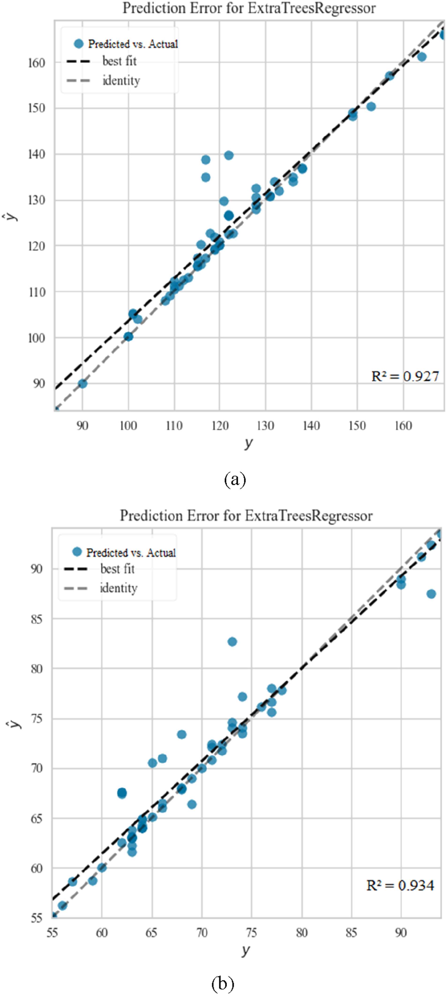
Comparative analysis of predicted (ŷ) Versus actual (y) values for BP estimation using ET: (a) illustrates the best result obtained for Systolic BP prediction, while (b) depicts the best result for Diastolic BP prediction.

We tested various hyperparameters using 10-fold cross-validation across all algorithms. The optimal hyperparameters of algorithms, which achieved favorable results for both SBP and DBP, are presented in Table 10.

Table 10.

Selected hyperparameters and their explored ranges for algorithms.

Algorithm	Hyperparameter	Selected value	Range explored
DT	criterion	squared_error	-
	max_depth	None	[None, 5, 10, 15, 20]
	max_features	None	[None, 0.1, 0.4, 0.7, 1.0]
	min_samples_leaf	1	[1, …, 10]
	min_samples_split	2	[2, …, 10]
RF	criterion	squared_error	-
	max_depth	None	[None, 5, 10, 15, 20]
	max_features	1.0	[0.1, 0.4, 0.7, 1.0]
	min_samples_leaf	1	[1, …, 10]
	min_samples_split	2	[2, …, 10]
	n_estimators	100	[50, …, 150]
ET	criterion	squared_error	-
	max_depth	None	[None, 5, 10, 15, 20]
	max_features	1.0	[None, 0.1, 0.4, 0.7, 1.0]
	min_samples_leaf	1	[1, …, 10]
	min_samples_split	2	[2, …, 10]
	n_estimators	100	[50, …, 150]
GB	criterion	friedman_mse	-
	max_depth	3	[None, 3, 5, 10, 15, 20]
	max_features	None	[None, 0.1, 0.4, 0.7, 1.0]
	min_samples_leaf	1	[1, …, 10]
	min_samples_split	2	[2, …, 10]
	n_estimators	100	[50, …, 150]
CB	loss_function	RMSE	-
CB	border_count	254	[64, 128, 254, 512]

In the second phase of our study, to ensure the reliability of our results, we redivided the data differently from the initial selection used for training and evaluation. This time, we set aside a distinct 20% of the data for testing, which was different from the previous split, leading to a corresponding change in the training dataset. We retrained and evaluated the models from scratch, utilizing the optimal hyperparameters identified through cross-validation in the initial phase, and employing the features selected by any of the feature selection methods used previously. The performance of each algorithm on the new test data for SBP and DBP are presented in Tables 11 and 12. It can be seen that the ET algorithm in combination with the SelectFromModel feature selection method (actually with the features that were selected by this method in the previous step) gives the best results. The comparison between the predicted output and the actual target for the best results is illustrated separately for SBP and DBP in Figure 9.

Table 11.

Performance comparison of algorithms for SBP using test data.

Model	Feature selection technique	MAE	MSE	RMSE	R²	MAPE
DT	SelectFromModel	3.19	72.66	8.52	0.82	0.02
	SelectKBest	6.63	163.0	12.77	0.61	0.05
	RFE	6.28	172.3	13.12	0.58	0.05
	SFS	2.94	51.36	7.16	0.87	0.02
	CFS	2.52	74.35	8.62	0.82	0.02
RF	SelectFromModel	5.74	78.42	8.85	0.81	0.04
	SelectKBest	6.28	86.84	9.31	0.79	0.05
	RFE	7.08	110.3	10.50	0.73	0.06
	SFS	6.04	71.64	8.64	0.82	0.04
	CFS	5.50	75.40	8.68	0.81	0.04
ET	SelectFromModel	2.55	29.33	5.41	0.93	0.02
	SelectKBest	3.38	59.58	7.71	0.85	0.02
	RFE	4.81	80.15	8.95	0.80	0.04
	SFS	2.49	33.67	5.80	0.91	0.02
	CFS	2.11	44.88	6.69	0.89	0.02
GB	SelectFromModel	6.65	97.35	9.86	0.76	0.05
	SelectKBest	6.81	111.1	10.54	0.73	0.05
	RFE	7.99	109.5	10.46	0.73	0.06
	SFS	6.67	85.71	9.25	0.79	0.05
	CFS	7.29	115.4	10.74	0.72	0.05
CB	SelectFromModel	4.19	46.36	6.80	0.88	0.03
	SelectKBest	4.53	65.03	8.06	0.84	0.03
	RFE	5.75	72.09	8.49	0.82	0.04
	SFS	4.52	47.32	6.87	0.88	0.03
	CFS	4.82	63.22	7.95	0.84	0.03

Table 12.

Performance comparison of algorithms for DBP using test data.

Model	Feature selection technique	MAE	MSE	RMSE	R²	MAPE
DT	SelectFromModel	1.71	25.50	5.05	0.78	0.02
	SelectKBest	3.14	65.00	8.06	0.44	0.04
	RFE	2.57	40.01	6.32	0.66	0.03
	SFS	3.00	43.45	6.59	0.63	0.04
	CFS	2.25	27.72	5.26	0.76	0.03
RF	SelectFromModel	3.43	25.89	5.08	0.78	0.04
	SelectKBest	3.12	25.47	5.04	0.78	0.04
	RFE	3.84	33.25	5.76	0.71	0.05
	SFS	3.93	29.76	5.45	0.74	0.05
	CFS	3.39	30.49	5.52	0.74	0.04
ET	SelectFromModel	1.40	8.29	2.87	0.93	0.01
	SelectKBest	1.65	12.45	3.52	0.89	0.02
	RFE	2.61	19.02	4.36	0.84	0.03
	SFS	1.56	8.81	2.96	0.92	0.02
	CFS	2.09	22.14	4.70	0.81	0.03
GB	SelectFromModel	3.92	32.70	5.71	0.72	0.05
	SelectKBest	4.08	35.72	5.97	0.69	0.05
	RFE	4.30	36.00	6.00	0.69	0.06
	SFS	4.18	37.77	6.14	0.67	0.05
	CFS	4.44	40.16	6.33	0.66	0.06
CB	SelectFromModel	2.36	14.31	3.78	0.87	0.03
	SelectKBest	2.65	17.44	4.17	0.85	0.03
	RFE	3.62	29.43	5.42	0.75	0.05
	SFS	2.89	17.59	4.19	0.85	0.04
	CFS	3.50	27.46	5.24	0.76	0.05

Figure 9.

Comparative analysis of predicted (ŷ) Versus Actual (y) Values for BP Estimation Using ET: (a) illustrates the best result obtained for Systolic BP prediction, while (b) depicts the best result for Diastolic BP prediction.

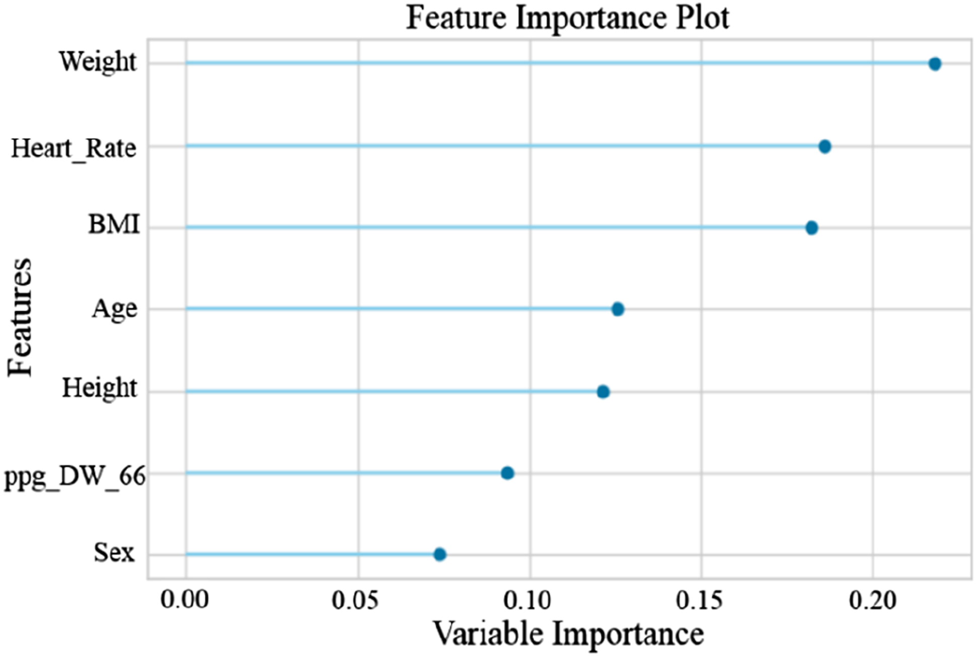
The findings of the experiments emphasize the effectiveness of the ET algorithm in BP estimation. The SelectFromModel feature selection technique focuses on the most relevant and distinct aspects of the data, and by identifying 10 key features for SBP and seven critical features for DBP from the set of extracted features, it results in the ET algorithm achieving the resultant outcomes. The 10 features selected by the SelectFromModel feature selection method for SBP include Age, Heart rate, BMI, Weight, Sex, Height, ppg_DW_SW_75, ppg_DW_SW_50, Cerebrovascular disease, and Diabetes. Additionally, seven features selected by this method for DBP include Weight, Heart Rate, BMI, Age, Height, ppg_DW_66, and Sex.

By employing the recursive feature elimination with cross validation (RFECV) method, we assessed the significance of each feature for SBP and DBP, and their corresponding graphs are depicted in Figures 10 and 11. As evident, Age is the most critical feature in estimating SBP,^70–74 while Weight plays a significant role in DB^75–79 estimation. These results align with the findings of several mentioned studies. It should be noted that the scale of variable importance in Figures 10 and 11 is normalized between 0 and 1, where a value of 1 indicates the most important feature relative to the others in the model. This does not imply that the feature is perfect or flawless, but rather that it contributes the most to the prediction accuracy compared with other features. Values closer to 0 indicate features with less relative impact, though they may still carry useful information.

Figure 10.

Importance of ten features for estimating SBP – A graphical representation highlighting the significance of various features in the accurate estimation of SBP.

Figure 11.

Importance of seven features for estimating DBP – A graphical representation highlighting the significance of various features in the accurate estimation of DBP.

Discussion

In general, comparing similar works in this field is challenging due to variations in databases, applied methods, and evaluation criteria. Some studies reported the lowest errors using small selected subsets of public or private data, while others worked on large-scale databases with higher error rates. Looking at each of the related works in Table 13, Kim et al.³⁹ conducted a comparison between ANN and multiple regression as methods for BP estimation; however, their study was confined to a mere 45 subjects. They utilized both PPG and ECG signals, and did not estimate DBP. In their study, Kachuee et al.⁴⁰ introduced an approach that utilizes physiological parameters, ML, and signal processing algorithms, employing the PTT method along with specific time-domain PPG features. It’s worth noting that they utilized the MIMIC II dataset, which differs from the dataset used in our work. From our perspective, the MIMIC dataset lacked well-rounded distribution in various aspects. Considering that a large number of people were examined, it has a high error. Cattioli et al.⁴¹ introduced a BP estimation algorithm using a small dataset (34 recordings for 25 subjects), incorporating both ECG and PPG signals. Zhang et al.⁴³ applied the SVM and neural network approach, achieving better results with SVM compared to their previous work on 32 subjects.

Table 13.

Comparing the performance with prior research.

Authors	Database	Signals	Method	Performance criteria	SBP	DBP
Kim et al.³⁹	180 recordings (45 subjects)	PPG & ECG	Multiple nonlinear regression	MAE	5.67	-
				MSE	-	-
				RMSE	-	-
				R²	-	-
				MAPE	-	-
Kim et al.³⁹	180 recordings (45 subjects)	PPG & ECG	ANN	MAE	4.53	-
				MSE	-	-
				RMSE	-	-
				R²	-	-
				MAPE	-	-
Kachuee et al.⁴⁰	MIMIC II (1000 subjects)	PPG & ECG	SVM	MAE	12.38	6.34
				MSE	-	-
				RMSE	-	-
				R²	-	-
				MAPE	-	-
Cattivelli et al.⁴¹	MIMIC (25 subjects)	PPG & ECG	Proprietary algorithm	MAE	-	-
				MSE	70.05	35.08
				RMSE	-	-
				R²	-	-
				MAPE	-	-
Zhang et al.⁴³	32 patients	Only PPG	ANN	MAE	11.89	8.83
				MSE	-	-
				RMSE	-	-
				R²	-	-
				MAPE	-	-
Zhang et al.⁴³	32 patients	Only PPG	SVM	MAE	11.64	7.62
				MSE	-	-
				RMSE	-	-
				R²	-	-
				MAPE	-	-
Su et al.⁴⁵	84 subjects	PPG & ECG	LSTM	MAE	-	-
				MSE	-	-
				RMSE	3.73	2.43
				R²	-	-
				MAPE	-	-
Slapničar et al.⁴⁷	MIMIC III (510 subjects)	Only PPG	DL (Spectro-temporal ResNet)	MAE	9.43	6.88
				MSE	-	-
				RMSE	-	-
				R²	-	-
				MAPE	-	-
Zadi et al.⁸⁰	15 subjects	Only PPG	ARMA models	MAE	-	-
				MSE	-	-
				RMSE	6.49	4.33
				R²	-	-
				MAPE	-	-
Chowdhury et al.²⁸	PPG-BP (222 signals, 126 subjects)	Only PPG	GPR	MAE	3.02	1.74
				MSE	45.49	12.89
				RMSE	6.74	3.59
				R²	0.90	0.92
				MAPE	-	-
Our study	PPG-BP (282 signals, 137 subjects)	Only PPG	ET	MAE	2.54	1.37
				MSE	27.22	7.14
				RMSE	5.21	2.65
				R²	0.93	0.93
				MAPE	0.02	0.01

Su et al.⁴⁵ used DL, in their work they used both PPG and ECG signals of a small database and obtained low error due to the small number of subjects. Slapničar et al.⁴⁷ worked with the MIMIC III dataset and achieved reasonable estimation accuracy using DL spectro-temporal ResNet algorithm. Zadi et al.⁸⁰ used a very small dataset (only 15 people) to calculate SBP and DBP, and estimates were obtained from the PPG signal as input to fifth-order autoregressive moving average (ARMA) models. Chowdhury et al.²⁸ used our selected dataset but considered fewer people and signals. They achieved their results by extracting features from signals and using the GPR algorithm, while we were able to achieve better results with more people and signals and different and fewer inputs and a distinct algorithm.

As far as we know, no work has extracted all of our features and achieved such a low error rate using the SelectFromModel feature selection method and the ET machine learning algorithm. Table 13 provides a comparative summary of the mentioned works with our study based on evaluation parameters: MAE, MSE, RMSE, R², and MAPE (The results reported in Table 13 are the average results of two phases of our study).

It is essential to emphasize that the standard evaluation of BP measuring devices, as proposed by the Association for the Advancement of Medical Instrumentation (AAMI),^28,81 was conducted with high accuracy in our study. As indicated in Table 14, the AAMI standard deems the results of the ET algorithm for both SBP and DBP acceptable.

Table 14.

Comparison of study results with the AAMI standard for BP measurements.

		Mean (mmHg)	SD (mmHg)	Subject
AAMI⁸¹	BP	≤5	≤8	≥85
Our study	SBP MAE	2.54	4.54	137
Our study	DBP MAE	1.37	2.27	137

In general, in this research, in addition to achieving better results, our goal was to eliminate the limitations of previous studies. Compared to some studies, we examined a larger number of participants and the selected data set shows a good representation of people in different age groups, including healthy and unhealthy people of both sexes. Furthermore, we used only PPG signals, simplifying the complexities encountered in a series of studies. Finally, we used ML algorithms, which require less training time compared to DL models.

Our research effectively learned the underlying algorithms and infrastructures in the dataset using the selected features as input to the ET algorithm. The success of the ET algorithm can be attributed to several factors, including:

(1) ET is an ensemble learning method that builds several DTs and combines their predictions. This helps reduce overfitting and improve generalization to new and unseen data.

(2) The algorithm uses a random subset of features for each DT, which increases diversity among trees and can improve performance.

(3) PPG signals can still have noise despite the pre-processing steps, and this affects the extracted features. Ensemble methods such as ET are generally robust against noisy data because they consider multiple models and can effectively deal with outliers.

(4) PPG signals often show complex and non-linear patterns. DT-based algorithms, including ET, are able to capture nonlinear relationships between features and the target variable, making them suitable for such data.

Additionally, SelectFromModel helped enhance the performance by selecting only the most relevant features from the dataset, eliminating irrelevant or less impactful ones. This further optimized the model by ensuring that it focuses on the most important features, improving both its efficiency and accuracy.

This study demonstrates promising results in BP estimation using PPG signals. However, there are several aspects that can be explored in future research to further enhance the model’s applicability and generalizability.

First, this study primarily utilizes the Figshare database as the primary data source. While the dataset provides a reasonable level of diversity, it may not fully encompass all demographic groups or rare clinical conditions. Although the proposed model has shown strong performance under the given conditions, future work could benefit from the inclusion of larger, more representative datasets that capture a broader range of demographic and clinical characteristics. Incorporating datasets that represent diverse populations, including various age groups, ethnicities, and patients with rare conditions, would help assess the model’s robustness and improve its performance across different clinical scenarios.

Additionally, this study focuses on BP estimation using PPG signals in controlled environments, where factors such as sensor calibration and signal quality are optimized. In real-world applications, however, challenges such as sensor quality, motion artifacts, noise levels, and skin-tone variability can impact signal accuracy and lead to less reliable measurements. For instance, poor sensor calibration or suboptimal skin contact can introduce inaccuracies, while noise from environmental factors, such as ambient light or electrical interference, can degrade signal fidelity. Furthermore, variations in skin tone can affect the absorption and reflection of light, especially in devices using light-based sensors, which could result in significant variations in signal strength and quality across different individuals.

To further improve the model’s performance, it is crucial to evaluate the system’s effectiveness in real-world, less controlled settings. This includes addressing challenges related to motion artifacts, sensor calibration, and noise interference, which are inherent in everyday usage. Moreover, future work will focus on incorporating datasets annotated for skin tone and ethnicity to systematically investigate the impact of optical and physiological diversity on PPG signal quality and BP estimation accuracy. External validation using diverse datasets that capture real-world variability could help affirm the model’s translational value and demonstrate its effectiveness across various populations and environmental conditions.

While the limitations mentioned above do not impact the validity of our current findings, addressing these challenges in future studies could significantly enhance the generalizability, robustness, and practical utility of the proposed approach.

Conclusions

In this research, the authors have proposed and implemented a methodology for estimating SBP and DBP using features extracted from the PPG signal and ML algorithms. The research effectively demonstrates the estimation of patients’ BP without resorting to cuff-based pressure measurement or invasive techniques, thereby overcoming the drawbacks associated with both invasive and non-invasive cuff-based measurements.

The entire process, encompassing the preprocessing of PPG fingertip signals, feature extraction, feature reduction, and the training and evaluation of algorithms, was comprehensively discussed. Various preprocessing techniques were applied to the raw signals. This system used time-domain, frequency-domain and statistical features along with demographic data and features obtained from different formulas. To address computational complexity, different feature selection methods were utilized. The SBP and DBP were trained separately because they often had different key properties. Ten different ML algorithms were trained and evaluated for SBP and DBP. The combination of the SelectFromModel feature selection method and the ET machine learning algorithm yielded the most favorable outcomes. The ET algorithm achieved a noteworthy R² score of 0.93 for both SBP and DBP.

In future work, DL algorithms can be used with larger datasets to generate a better prediction model. The trained model can be used in the development of prototypes for wearable or portable BP monitoring devices based on commercial light-based sensors, such as PPG, to estimate blood pressure. Such a system can contribute to continuous BP monitoring and help prevent critical health conditions due to sudden changes.

Footnotes

ORCID iDs

Bahram Tarvirdizadeh

Khalil Alipour

Ethical considerations

Given the nature of this research, which involved the analysis of existing, publicly available data without direct involvement of human or animal subjects, formal ethical approval was not required.

Funding

The authors received no financial support for the research, authorship, and/or publication of this article.

Declaration of conflicting interests

The authors declared no potential conflicts of interest with respect to the research, authorship, and/or publication of this article.

References

Fuchs

Whelton

. High blood pressure and cardiovascular disease. Hypertension 2020; 75(2): 285–292.

Koivistoinen

Lyytikäinen

Aatola

, et al. Pulse wave velocity predicts the progression of blood pressure and development of hypertension in young adults. Hypertension 2018; 71(3): 451–456.

World Health Organization . Hypertension [Internet]. WHO, 2023. [cited 2024 Jan 21]. Available from: https://www.who.int/news-room/fact-sheets/detail/hypertension

Ribas Ripoll

Wojdel

Romero

, et al. ECG assessment based on neural networks with pretraining. Appl Soft Comput 2016; 49: 399–406.

Roth

Forouzanfar

Moran

, et al. Demographic and epidemiologic drivers of global cardiovascular mortality. N Engl J Med 2015; 372(14): 1333–1341.

Meidert

Saugel

. Techniques for non-invasive monitoring of arterial blood pressure. Front Med 2018; 4: 231.

Goldberg

Levy

. New approaches to evaluating and monitoring blood pressure. Curr Hypertens Rep 2016; 18(6): 49.

Konstantinidis

Iliakis

Tatakis

, et al. Wearable blood pressure measurement devices and new approaches in hypertension management: the digital era. J Hum Hypertens 2022; 36(11): 945–951.

Tomitani

Hoshide

Kario

. Novel blood pressure monitoring methods: perspectives for achieving “perfect 24-h blood pressure management”. Hypertens Res 2023; 46(8): 2051–2053.

10.

Al Fahoum

Abu Al-Haija

Alshraideh

. Identification of coronary artery diseases using photoplethysmography signals and practical feature selection process. Bioengineering 2023; 10(2): 249.

11.

Teng

Zhang

. Continuous and noninvasive estimation of arterial blood pressure using a photoplethysmographic approach. In: Proceedings of the 25th Annual International Conference of the IEEE Engineering in Medicine and Biology Society (IEEE Cat No 03CH37439). IEEE, 2003.

12.

McCombie

Reisner

Asada

. Adaptive blood pressure estimation from wearable PPG sensors using peripheral artery pulse wave velocity measurements and multi-channel blind identification of local arterial dynamics. In: 2006 International Conference of the IEEE Engineering in Medicine and Biology Society. IEEE.

13.

Zhang

Wei

. A LabVIEW based measure system for pulse wave transit time. In: 2008 International Conference on Information Technology and Applications in Biomedicine. IEEE, 2008.

14.

Liu

Xiao

, et al. A novel interpretable feature set optimization method in blood pressure estimation using photoplethysmography signals. Biomed Signal Process Control 2023; 86: 105184.

15.

Poon

Zhang

. Cuff-less and noninvasive measurements of arterial blood pressure by pulse transit time. In: 2005 IEEE engineering in medicine and biology 27th annual conference. IEEE, 2006.

16.

Loh

Faust

, et al. Application of photoplethysmography signals for healthcare systems: an in-depth review. Comput Methods Progr Biomed 2022; 216: 106677.

17.

Castaneda

Esparza

Ghamari

, et al. A review on wearable photoplethysmography sensors and their potential future applications in health care. Int J Biosens Bioelectron 2018; 4(4): 195–202.

18.

Hasanpoor

Motaman

Tarvirdizadeh

, et al. Stress detection using ppg signal and combined deep cnn-mlp network. In: 2022 29th National and 7th International Iranian Conference on Biomedical Engineering (ICBME). IEEE, 2022.

19.

Pankaj

Kumar

Komaragiri

, et al. A review on computation methods used in photoplethysmography signal analysis for heart rate estimation. Arch Comput Methods Eng 2022; 29(2): 921–940.

20.

Mohammadi

Tarvirdizadeh

Alipour

, et al. Blood pressure estimation through photoplethysmography and machine learning models. In: 2023 9th International Conference on Control, Instrumentation and Automation (ICCIA). IEEE, 2023.

21.

Mohammadi

Tarvirdizadeh

Alipour

, et al. Noninvasive blood pressure classification based on photoplethysmography using machine learning techniques. In: 2024 32nd International Conference on Electrical Engineering (ICEE). IEEE, 2024.

22.

Mohammadi

Tarvirdizadeh

Alipour

, et al. Cuff-less blood pressure monitoring via PPG signals using a hybrid CNN-BiLSTM deep learning model with attention mechanism. Sci Rep 2025; 15(1): 22229.

23.

Elgendi

. PPG signal analysis: an introduction using MATLAB®. CRC Press, 2020.

24.

Liang

Chen

Liu

, et al. A new, short-recorded photoplethysmogram dataset for blood pressure monitoring in China. Sci Data 2018; 5(1): 180020–180027.

25.

Saleh

Salaheldin

Ismail

, et al. Classification of anemic condition based on photoplethysmography signals and clinical dataset. Biomedical Engineering/Biomedizinische Technik 2025; 70: 359–370.

26.

Tamura

Maeda

Sekine

, et al. Wearable photoplethysmographic sensors—past and present. Electronics 2014; 3(2): 282–302.

27.

Bashkatov

Genina

Kochubey

, et al. Optical properties of human skin, subcutaneous and mucous tissues in the wavelength range from 400 to 2000 nm. J Phys D Appl Phys 2005; 38(15): 2543–2555.

28.

Chowdhury

Shuzan

MNI

Chowdhury

, et al. Estimating blood pressure from the photoplethysmogram signal and demographic features using machine learning techniques. Sensors 2020; 20(11): 3127.

29.

Martínez

Howard

Abbott

, et al.

Can photoplethysmography replace arterial blood pressure in the assessment of blood pressure?

J Clin Med 2018; 7(10): 316.

30.

Finnegan

Davidson

Harford

, et al. Features from the photoplethysmogram and the electrocardiogram for estimating changes in blood pressure. Sci Rep 2023; 13(1): 986.

31.

Xing

Zhang

, et al. An unobtrusive and calibration-free blood pressure estimation method using photoplethysmography and biometrics. Sci Rep 2019; 9(1): 8611.

32.

Rundo

Ortis

Battiato

, et al. Advanced bio-inspired system for noninvasive cuff-less blood pressure estimation from physiological signal analysis. Computation 2018; 6(3): 46.

33.

Park

Seok

Kim

S-S

, et al. Photoplethysmogram analysis and applications: an integrative review. Front Physiol 2022; 12: 808451.

34.

Elgendi

. On the analysis of fingertip photoplethysmogram signals. Curr Cardiol Rev 2012; 8(1): 14–25.

35.

Gaurav

Maheedhar

Tiwari

, et al. Cuff-less PPG based continuous blood pressure monitoring—A smartphone based approach. In: 2016 38th annual international conference of the IEEE engineering in medicine and biology society (EMBC). IEEE, 2016.

36.

Liu

L-M

. Cuffless blood pressure estimation based on photoplethysmography signal and its second derivative. International Journal of Computer Theory and Engineering 2017; 9(3): 202–206.

37.

Rong

. A multi-type features fusion neural network for blood pressure prediction based on photoplethysmography. Biomed Signal Process Control 2021; 68: 102772.

38.

Mohamed

Fletcher

Yongbo

, et al. The use of photoplethysmography for assessing hypertension. npj Digital Medicine 2019; 2(1): 60.

39.

Kim

Cho

, et al. Comparative study on artificial neural network with multiple regressions for continuous estimation of blood pressure. In: 2005 IEEE Engineering in Medicine and Biology 27th Annual Conference. IEEE, 2006.

40.

Kachuee

Kiani

Mohammadzade

, et al. Cuff-less high-accuracy calibration-free blood pressure estimation using pulse transit time. In: 2015 IEEE international symposium on circuits and systems (ISCAS). IEEE, 2015.

41.

Cattivelli

Garudadri

. Noninvasive cuffless estimation of blood pressure from pulse arrival time and heart rate with adaptive calibration. In: 2009 Sixth international workshop on wearable and implantable body sensor networks. IEEE, 2009.

42.

Xing

Sun

. Optical blood pressure estimation with photoplethysmography and FFT-based neural networks. Biomed Opt Express 2016; 7(8): 3007–3020.

43.

Zhang

Feng

. A SVM method for continuous blood pressure estimation from a PPG signal. In: Proceedings of the 9th international conference on machine learning and computing, 2017.

44.

Saad

Saleh

Wahed

, et al. A combined deep learning-regression paradigm for echocardiography-based left ventricle ejection fraction prediction. In: 2024 6th Novel Intelligent and Leading Emerging Sciences Conference (NILES). IEEE, 2024.

45.

Ding

X-R

Zhang

Y-T

, et al. Long-term blood pressure prediction with deep recurrent neural networks. In: 2018 IEEE EMBS International conference on biomedical & health informatics (BHI). IEEE, 2018.

46.

Gotlibovych

Crawford

Goyal

, et al. End-to-end deep learning from raw sensor data: atrial fibrillation detection using wearables. arXiv preprint arXiv:180710707 2018.

47.

Slapničar

Mlakar

Luštrek

. Blood pressure estimation from photoplethysmogram using a spectro-temporal deep neural network. Sensors 2019; 19(15): 3420.

48.

Liang

Elgendi

Chen

, et al. An optimal filter for short photoplethysmogram signals. Sci Data 2018; 5(1): 180076.

49.

Pollreisz

TaheriNejad

. Detection and removal of motion artifacts in PPG signals. Mob Netw Appl 2022; 27(2): 728–738.

50.

Millasseau

Kelly

Ritter

, et al. Determination of age-related increases in large artery stiffness by digital pulse contour analysis. Clin Sci 2002; 103(4): 371–377.

51.

Elgendi

Norton

Brearley

, et al. Detection of a and b waves in the acceleration photoplethysmogram. Biomed Eng Online 2014; 13(1): 139.

52.

Chatterjee

Roy

. PPG based heart rate algorithm improvement with Butterworth IIR Filter and Savitzky-Golay FIR Filter. In: 2018 2nd International conference on electronics, materials engineering & Nano-technology (IEMENTech). IEEE, 2018.

53.

Otsuka

Kawada

Katsumata

, et al. Utility of second derivative of the finger photoplethysmogram for the estimation of the risk of coronary heart disease in the general population. Circ J 2006; 70(3): 304–310.

54.

Sun

Peeters

Bezemer

, et al. Finger and forehead photoplethysmography-derived pulse-pressure variation and the benefits of baseline correction. J Clin Monit Comput 2019; 33(1): 65–75.

55.

Maxwell

. A treatise on electricity and magnetism. Clarendon Press, 1873.

56.

BIOBSS . Welcome to BIOBSS's documentation! BIOBSS, 2023. [cited 2024 Jan 27]. Available from: https://biobss.readthedocs.io/en/latest/

57.

Scikit-learn developers . Feature selection [Internet]. Scikit-learn 1.4.0 Documentation; 2024. [cited 2024 Jan 27]. Available from: https://scikit-learn.org/stable/modules/feature_selection.html

58.

Hall

. Correlation-based feature selection for machine learning [dissertation on the Internet]. Hamilton (New Zealand): University of Waikato, 1999. [cited 2024 Jan 27]. Available from: https://researchcommons.waikato.ac.nz/handle/10289/15043

59.

Scikit-learn developers . Cross-validation: evaluating estimator performance [Internet]. Scikit-learn 1.4.0 Documentation; 2024, [cited 2024 Jan 27]. Available from: https://scikit-learn.org/stable/modules/cross_validation.html

60.

Scikit-learn developers . Regression metrics [Internet]. Scikit-learn 1.4.0 Documentation; 2024. [cited 2024 Jan 27]. Available from: https://scikit-learn.org/stable/modules/model_evaluation.html#regression-metrics

61.

Loh

. Classification and regression trees. WIREs Data Min & Knowl 2011; 1(1): 14–23.

62.

Scikit-learn developers . sklearn.tree.DecisionTreeRegressor [Internet]. Scikit-learn 1.4.0 Documentation; 2024. [cited 2024 Jan 27]. Available from: https://scikit-learn.org/stable/modules/generated/sklearn.tree.DecisionTreeRegressor.html

63.

Breiman

. Random forests. Mach Learn 2001; 45(1): 5–32.

64.

Scikit-learn developers . sklearn.ensemble.RandomForestRegressor [Internet]. Scikit-learn 1.4.0 Documentation; 2024. [cited 2024 Jan 27]. Available from: https://scikit-learn.org/stable/modules/generated/sklearn.ensemble.RandomForestRegressor.html

65.

Geurts

Ernst

Wehenkel

. Extremely randomized trees. Mach Learn 2006; 63(1): 3–42.

66.

Scikit-learn developers . sklearn.ensemble.ExtraTreesRegressor [Internet]. Scikit-learn 1.4.0 Documentation; 2024. [cited 2024 Jan 27]. Available from: https://scikit-learn.org/stable/modules/generated/sklearn.ensemble.ExtraTreesRegressor.html

67.

Scikit-learn developers . sklearn.ensemble.GradientBoostingRegressor [Internet]. Scikit-learn 1.4.0 Documentation; 2024. [cited 2024 Jan 27]. Available from: https://scikit-learn.org/stable/modules/generated/sklearn.ensemble.GradientBoostingRegressor.html

68.

Dorogush

Ershov

Gulin

. CatBoost: gradient boosting with categorical features support. arXiv preprint arXiv:181011363. 2018.

69.

Salaheldin

Abdel Wahed

Talaat

, et al. An evaluation of AI-based methods for papilledema detection in retinal fundus images. Biomed Signal Process Control 2024; 92: 106120.

70.

Singh

Nguyen

Kerndt

, et al. Physiology, blood pressure age related changes. 2019.

71.

Cheng

Zhang

, et al. Age-related changes in the risk of high blood pressure. Front Cardiovasc Med 2022; 9: 939103.

72.

Gurven

Blackwell

Rodríguez

, et al. Does blood pressure inevitably rise with age? Longitudinal evidence among forager-horticulturalists. Hypertension 2012; 60(1): 25–33.

73.

Pinto

. Blood pressure and ageing. Postgrad Med J 2007; 83(976): 109–114.

74.

Izzo

Levy

Black

. Importance of systolic blood pressure in older Americans. Hypertension 2000; 35(5): 1021–1024.

75.

Sabaka

Dukat

Gajdosik

, et al. The effects of body weight loss and gain on arterial hypertension control: an observational prospective study. Eur J Med Res 2017; 22(1): 43.

76.

Harsha

Bray

. Weight loss and blood pressure control (Pro). Hypertension 2008; 51(6): 1420–1425.

77.

Staessen

Fagard

Amery

. The relationship between body weight and blood pressure. J Hum Hypertens 1988; 2(4): 207–217.

78.

Fogari

Zoppi

Corradi

, et al. Effect of body weight loss and normalization on blood pressure in overweight non-obese patients with stage 1 hypertension. Hypertens Res 2010; 33(3): 236–242.

79.

Linderman

, et al. Association of body mass index with blood pressure among 1.7 million Chinese adults. JAMA Netw Open 2018; 1(4): e181271.

80.

Soltan Zadi

Alex

Zhang

, et al. Arterial blood pressure feature estimation using photoplethysmography. Comput Biol Med 2018; 102: 104–111.

81.

Association for the Advancement of Medical Instrumentation . Manual, electronic or automated sphygmomanometers. ANSI/AAMI SP10-2002/A1. Arlington, VA: Association for the Advancement of Medical Instrumentation, 2003.

Exploring the potential of five machine learning regression algorithms for noninvasive blood pressure estimation with photoplethysmography

Abstract

Keywords

Introduction

Material and methods

Database description and collection protocol

Preprocessing of PPG signals

Normalization

Filtering

Baseline correction

Feature extraction

Feature selection

SelectFromModel

SelectKBest

Recursive Feature Elimination

Sequential Feature Selection

Correlation-based Feature Selection

Machine learning algorithms

Mean absolute error

Mean squared error

Root mean squared error

R-squared

Mean absolute percentage error

Decision tree Regressor

Random forest Regressor

Extra trees Regressor

Gradient boosting Regressor

CatBoost Regressor

Results

Discussion

Conclusions

Footnotes

ORCID iDs

Ethical considerations

Funding

Declaration of conflicting interests

References