Sage Journals: Discover world-class research

Abstract

Re-sampling methods to solve class imbalance problems have shown to improve classification accuracy by mitigating the bias introduced by differences in class size. However, it is possible that a model which uses a specific re-sampling technique prior to Artificial neural networks (ANN) training may not be suitable for aid in classifying varied datasets from the healthcare industry. Five healthcare-related datasets were used across three re-sampling conditions: under-sampling, over-sampling and combi-sampling. Within each condition, different algorithmic approaches were applied to the dataset and the results were statistically analysed for a significant difference in ANN performance. The combi-sampling condition showed that four out of the five datasets did not show significant consistency for the optimal re-sampling technique between the f1-score and Area Under the Receiver Operating Characteristic Curve performance evaluation methods. Contrarily, the over-sampling and under-sampling condition showed all five datasets put forward the same optimal algorithmic approach across performance evaluation methods. Furthermore, the optimal combi-sampling technique (under-, over-sampling and convergence point), were found to be consistent across evaluation measures in only two of the five datasets. This study exemplifies how discrete ANN performances on datasets from the same industry can occur in two ways: how the same re-sampling technique can generate varying ANN performance on different datasets, and how different re-sampling techniques can generate varying ANN performance on the same dataset.

Keywords

re-sampling artificial intelligence no-free-lunch artificial neural networks healthcare

Introduction

Artificial intelligence (AI) applications in solving modern-day industrial problems have shown popular success across a wide range of healthcare regions, from clinical imaging¹ to big data genomics² and drug development,³ reporting billions of dollars’ worth of value.⁴ The rapid development of advanced technology and digitization of healthcare paved way for successful and intuitive AI applications in the present day compared to its fruition in the 1950s; where theoretical AI was ahead of its computer hardware counterparts.⁵ Artificial neural networks (ANNs) are a type of AI approach that have been typically used in the healthcare for diagnosis assistance or monitoring of diseases.⁶ Previous research has stated that ANNs increase computational efficiency in comparison to other predictive algorithms⁷ thus becoming a favoured approach in research methodology. However, ANNs do not independently take into account the overall data distribution, and could require re-sampling to be implemented in the dataset pre-processing stages^8,9 if classes are imbalanced.

Imbalanced classes introduce a type of data bias where the amount of data which teaches an AI system to make a specific prediction is unequal to the amount of data used for a separate prediction. The classifier would tend to ignore the minority class with the fewer amount of data, while focussing on increasing the accuracy of classifying the majority class with the larger amount of data.¹⁰ For instance, consider a predictive model trained to provide diagnostic aid for melanoma detection. Hospital databases contain more images that indicate the absence of melanoma over the presence of melanoma. Thus, consider the ratio of melanoma images to be 99:1. By using this dataset, a trained model would falsely report a predictive accuracy of near 99%. The reason this is false is because this result corresponds to the skew towards the melanoma absent classification and the percentage of predictive accuracy applies only to this class. Upon using the model to predict for melanoma present, the predictive accuracy drops significantly below 1% – when in fact, this is the principal classification that requires the highest predictive accuracy. The result of this flaw shows a tendency to the irrelevant events rather than relevant events, as they typically contain the larger amount of data,¹⁰ in a situation were producing a false negative (i.e. missing a diagnosis) is more costly than a false positive. Therefore, the re-sampling method is particularly useful with healthcare data as it often exhibits classification problems with imbalanced classes.⁸ This involves increasing minority classes or decreasing majority classes in order to balance the samples representing each class. A review study found that re-sampling was utilized in 29.6% of class imbalance problems in literature,¹¹ indicating that re-sampling is a popular method to solve class imbalances. Furthermore, electronic medical records have made it possible to investigate the effects of re-sampling on mitigating the problem. For example, previous literature has found success for AI systems in healthcare such as detecting cardiovascular risk,^12,13 detection of Alzheimer’s¹⁴ and detection of Parkinson’s.¹⁵

In current affairs, the most popular procurement of AI in healthcare is for the purposes of aid or assistance. One of the inherent difficulties of AI is the ability to adapt with ever-changing data; it is complicit to assume a single classification model would be capable of providing accurate results across a variety of different data types. If AI systems are utilized to solve problems that they were not designed to solve, the results provided are likely to be inaccurate and thus detrimental to any industrial application. The application of AI in the healthcare industry is an extremely high-risk and highly sensitive area. This is because the solutions are concerned with the health status of an individual, leaving little to no room for error. For example, consider a digital health company that would like to create an application to remotely obtain a patient’s vital signs through a camera lens using photoplethysmography (PPG).¹⁶ An AI system would have to take into account variability in conditions pertinent to the camera, network, lighting and client in real-world settings. If during development, the AI is not fed with a variability of data for these settings, it is possible that the application would either not work or provide inaccurate results. An example of this includes when AI systems are fed data obtained from experiments in a lab setting. Studies have shown PPG to be susceptible to motion artefacts¹⁷ and decrease performance with poor lighting,¹⁸ making it wholly impossible for restless¹⁹ or tremor-prone patients with low lighting at home to make use of the application, whilst at the same time would work perfectly for clients capable of being sedentary with access to decent lighting. It is important to highlight AI systems as not consistently being a one-fits-all solution. AI systems can be heavily influenced by training data, which in itself can be dynamic and multifaceted. That being said, there are considerable benefits from responsibly utilized AI in the healthcare industry. Research has found promising potential in the use of AI in preliminary diagnostic assistance,²⁰ home assessments²¹ and robot-assisted surgeries²² as a few examples. Given the correct precautions, these approaches could prospectively improve on the two most important expenses for hospitals and general practices – time and money.^23,24

In this paper, we demonstrate the importance of responsible AI when mitigating class imbalances, and how neglecting a data-driven approach to re-sampling could lead to sub-optimal predictions. The objective is to convey that the same re-sampling technique across different datasets and different re-sampling techniques on the same dataset is capable of producing different results of the overall ANN performance and subsequently effecting the value of the predictions. There are many existing studies which review re-sampling techniques specifically for healthcare-related domains (such as medical, or disease diagnosis)^11,25,26 and which review different approaches to re-sampling (under-, over- and combi-sampling – also known as middle- or hybrid-sampling).^11,27 Aside from re-sampling, cost-sensitive learning techniques are also effective in addressing the class imbalance problem. Cost-sensitive learning algorithms focus on manipulation at the classifier level rather than the data level (as re-sampling does) and assigns a cost to every misclassification made. Previous literature has shown that combining CSL and re-sampling methods can help reduce misclassification costs and improve classifier performance.²⁸ However, considering the gap in the literature, this study focuses on the algorithmic comparisons within re-sampling techniques (i.e. algorithms within over-sampling, under-sampling and combi-sampling), specifically on healthcare data; which has been seldom reported before.²⁹ Comparisons between the re-sampling techniques or between datasets themselves were not conducted in this study. The remainder of this paper is organized into the following sections: the Methodology section involves the datasets and approaches taken. The Numerical Results section explains the experimental set-up and experimental results. The paper ends with the Discussion and Conclusion, sections whereby the Conclusion also addresses the limitations of the paper and an overview of future work.

Methodology

This section describes the applied datasets, the structure to the experiments conducted and the design of the experimental protocol. A total of five healthcare-related datasets were obtained from the UCI Machine Learning Repository.³⁰ In Table 1, the characteristics of each dataset are displayed including the number of instances, ANN structure, data source (demographic) and labelling (expert guidance).

Table 1.

Characteristics of utilized datasets from the UCI Machine Learning Database.³⁰

Dataset	Instances	ANN Structure Input	ANN Structure Output
Breast cancer	699	9	2
Cardiotocography	2,126	21	3
EEG eye state	14,980	14	2
Heart disease	303	13	2
Parkinson’s	195	22	2
Dataset	Subjects	Demographic	Expert Guidance
Breast cancer	687	USA	Yes
Cardiotocography	6,000	Europe and Australia	Yes
EEG eye state	1	Germany	No
Heart disease	303	USA	Yes
Parkinson’s	31	US	Yes

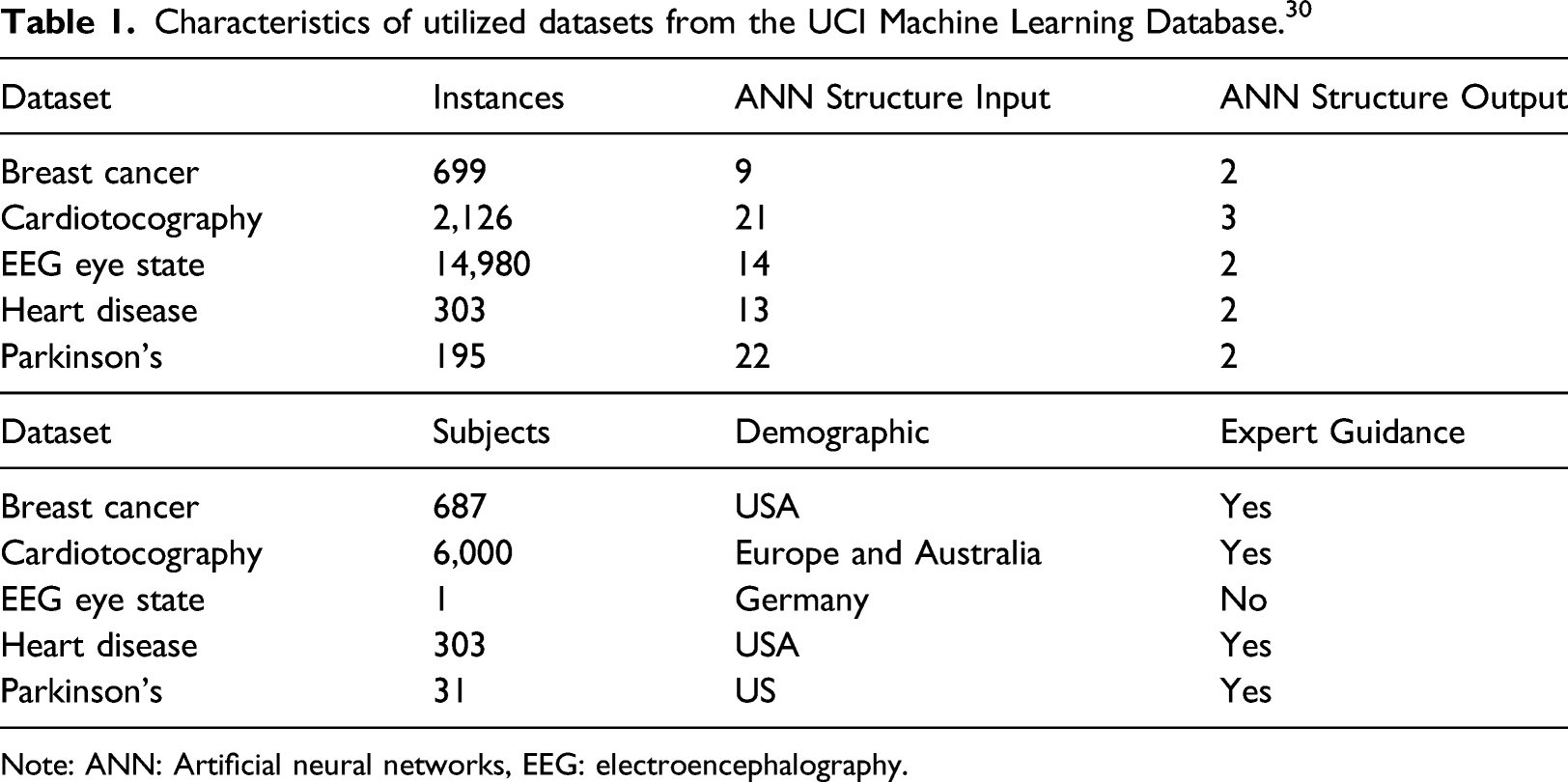
Note: ANN: Artificial neural networks, EEG: electroencephalography.

Dataset characteristics

The first step was to understand how each of the dataset characteristics contributes to the performance of an ANN. For example, in general, the larger the quantity of instances, the more comprehensive the knowledge is that’s obtained from the data³¹ leading to successful training of an ANN. Smaller datasets were included in this study to demonstrate the differences in performance that can occur with different dataset sizes. Similarly, the quality of data can determine successful applicability of an ANN in the real-world, which in these datasets are represented by the demographic and labelling. In the case for the Heart Disease and the Breast Cancer datasets, these contained instances of data which were incomplete. Having calculated approximately 2% of the dataset which had incomplete features, they were removed (pruned) from the dataset prior to ANN training and testing.^32–34 The demographic characteristic describes exactly how many participants and where in the world the data was extracted from, giving us an idea of which would be the most suitable setting in which to apply the ANN once it has been trained. The labelling characteristic allows us to understand how the classes were populated, that is, whether or not a medical professional, or else, determined that an instance belonged to a specific class based on their features, and precisely which features are deemed a necessary component of the instance (ANN structure). These features, are categorized into separate inputs, while the corresponding classifications are separated into outputs. As with the number of instances, it is ideal to recruit participants from a range of geographical sources and backgrounds.

Each characteristic is an important component of the datasets and can ultimately determine the route taken in building an AI system. These datasets were deliberately chosen due to their differences as it provides the necessary variability required to test whether the same re-sampling technique would produce different results across different datasets.

Experimental protocol

The re-sampling conditions included in this experiment were over-sampling (re-sampling smaller classes up to the majority class), under-sampling (re-sampling larger classes down to the minority class), combi-sampling (selecting a convergence point then utilizing both over-sampling and under-sampling techniques on the relevant classes) and a benchmark control of no re-sampling. Previous work implemented the combi-sampling technique using a single convergence point chosen at equal distances between the quantities of the minority and majority classes.³⁵ In this experiment, we extend this research by generating five convergence points, chosen at equal intervals from minority to majority class as illustrated in Table 2 and Figure 1.

Table 2.

Majority and minority class size characteristics from each dataset. Convergence point values represent convergence targets for the combi-sampling conditions in each dataset.

Dataset	Minority	Intermediate class			Majority
Breast cancer	239	-			444
Cardiotocography	176	295			1,655
EEG eye state	6,723	-			8,257
Heart disease	137	-			160
Parkinson’s	48	-			147
Dataset	Convergence point (combi-sampling)
	1	2	3	4	5
Breast cancer	264	315	341	366	418
Cardiotocography	453	730	915	1,192	1,470
EEG eye state	6,914	7,202	7,490	7,777	8,257
Heart disease	139	145	148	151	157
Parkinson’s	66	84	97	115	134

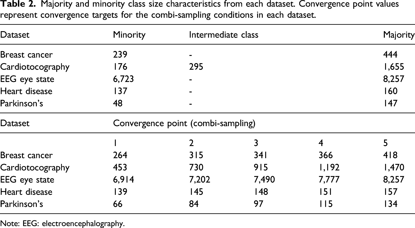
Note: EEG: electroencephalography.

Figure 1.

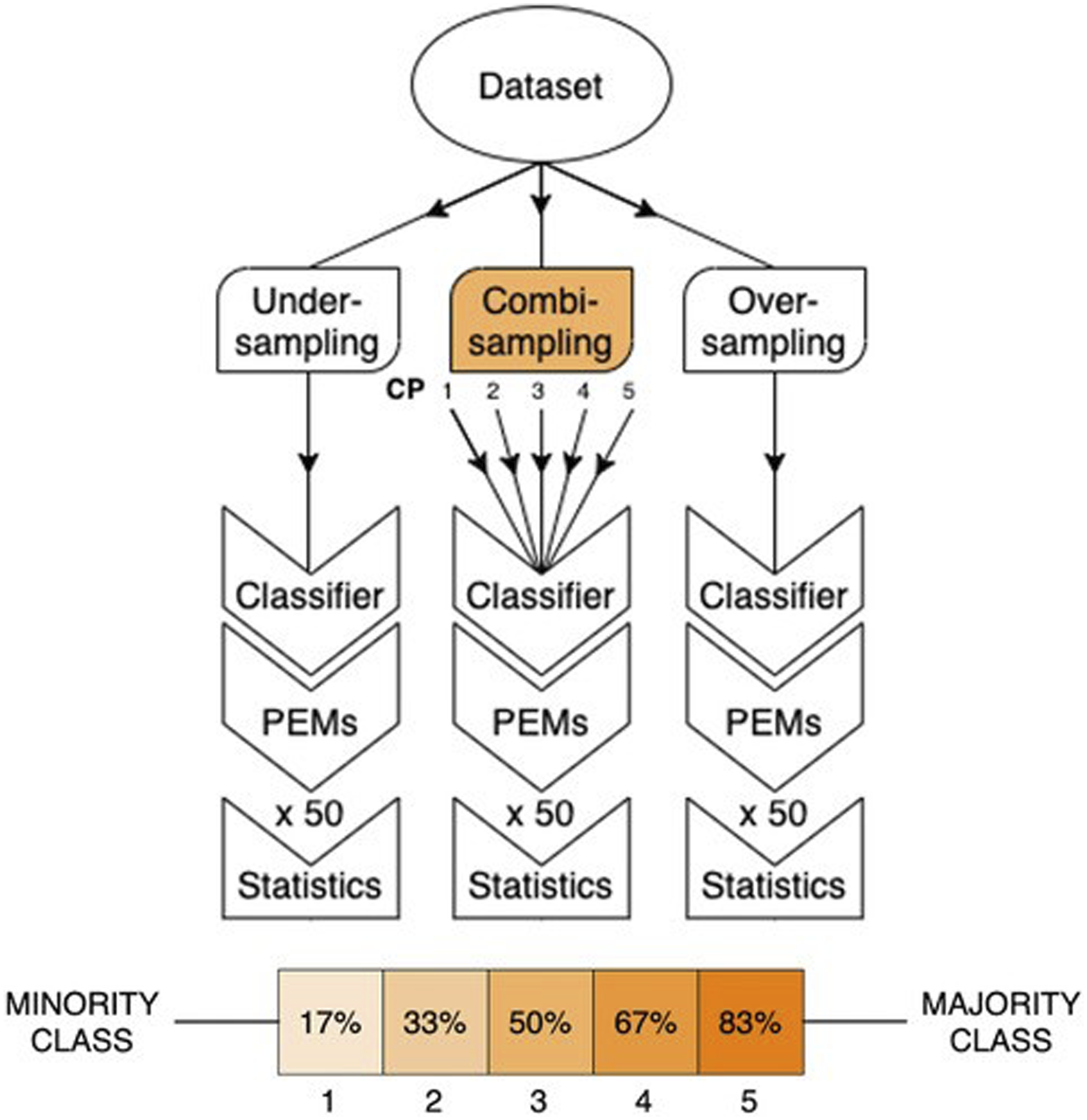
Flowchart graph to illustrate the methodology implemented for each of the re-sampling techniques and convergence points (CP).

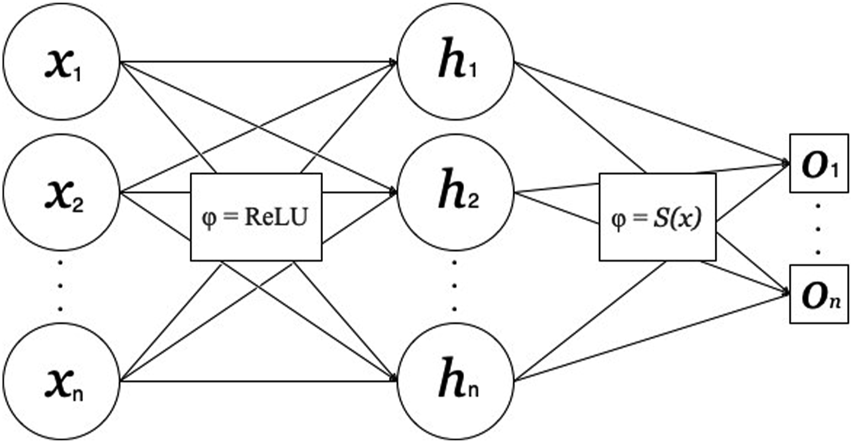
The ANN architecture was made up of an input, hidden and output layer, with the number of input nodes respective of the number of features for each dataset and similarly the number of output nodes respective of the number of classifications Figure 3. This architecture mimics previous procedures involving re-sampling comparisons, specifically involving combi-sampling.³⁵ A single hidden layer with node quantity identical to the input layer was suitable for this experiment.^36,37 An optimizer and loss function were defined for the learning process of the ANN, which was set up using a supervised learning approach. The aim of a loss function is to penalize incorrect predictions made by the ANN during training and successful ANN performance is contingent upon reducing the value of the loss function.³⁸ The optimizer carries out the learning process of updating weights and biases of the ANN (values produced between nodes which carry the patterns from input to output).³⁹ The datasets themselves were evaluated during the selection process of the loss and optimizer functions. For instance, because each dataset consisted of binary classifications, that is, [0 1] and [1 0] or in the case of Cardiotocography, [1 0 0], [0 1 0] and [0 0 1], research suggests that binary cross-entropy was the best suited for the ANN system of this experiment.⁴⁰ Furthermore, a majority of the datasets contain features which were measured on different scales, for example the Heart Disease dataset includes features of cholesterol level, resting blood pressure, age and sex. According to previous research, datasets of this type respond well to an optimizer function known as Adagrad, a gradient descent algorithm which is well-known for dealing with varying data sources within datasets.⁴¹ Each dataset was separated into training and testing subsets, 70% and 30%, respectively,^42–44 where the training subset was used for the learning process of the ANN and the testing subset acted as ‘unseen’ data to extract the performance of the trained ANN.

To determine the effect of each re-sampling condition on the ANN, performance evaluation measures (PEMs) were taken post-training. By implementing more than one PEM, we were able to gain more insight into performance of the ANN model ^45–47 above utilizing only one or two of the four main metrics: sensitivity, specificity, precision and recall. Significance testing of PEMs were conducted between each method in the re-sampling conditions, and each with the benchmark control.

Numerical results

This section describes the experimental results and is divided into two subsections. The first subsection describes the computational set-up defined by the experimental protocol and the second subsection describes the results of each re-sampling experiment arranged by the individual datasets.

Experimental set-up

Re-sampling techniques

An illustration of the 3 different re-sampling techniques used in this experiment is shown in Figure 2. To achieve over-sampling and under-sampling, 2 different algorithm methods were used within each condition. For combi-sampling, each algorithm from the over- and under-sampling techniques were used in conjunction with each other to produce 4 approaches. There were two general technical themes to re-sampling. The first technique was to utilize the existing feature space to derive newly generated datapoints.⁴⁸ These datapoints then acted as the new, re-sampled dataset under-sampled to the minority class. The second technique was to select the existing datapoints from the existing feature space to act as the new, re-sampled dataset until the dataset was the same size as the minority class.⁴⁸

Figure 2.

Diagram illustration using two datasets of different original sizes for the re-sampling techniques: (a) over-sampling, (b) under-sampling and (c) combi-sampling.

Figure 3.

Illustration of the Artificial neural networks architecture used in each re-sampling approach. Number (n) of input (x), hidden (h) and output (o) nodes correspond to the number of features and classes per dataset, respectively. Activation functions demonstrated between layers.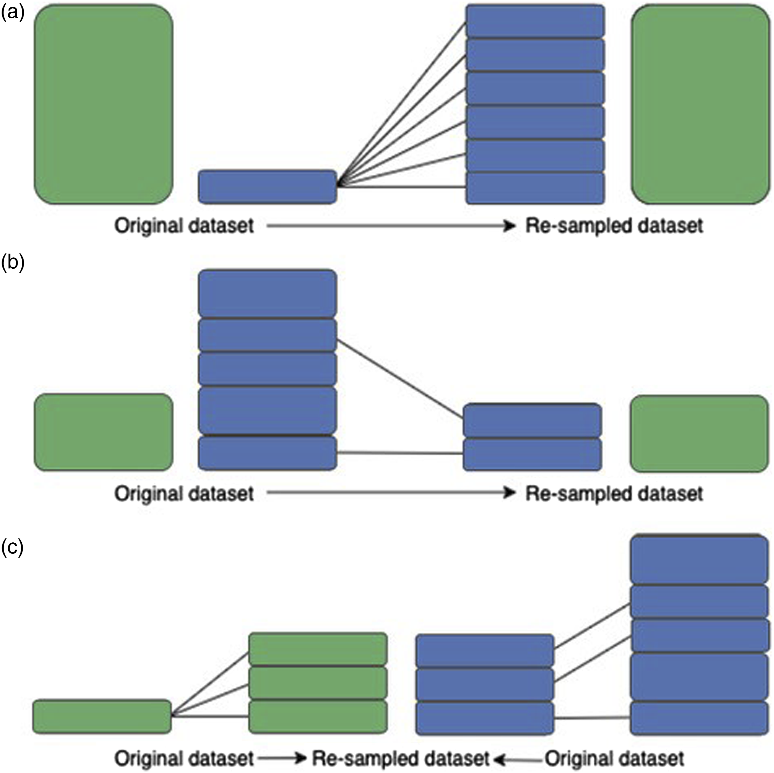

For the under-sampling conditions, both techniques were used – the Cluster Centroids (CC) algorithm, generated new datapoints and the Near Miss (NM) algorithm, which selected existing datapoints. In the over-sampling conditions, the re-sampling algorithms implemented were ADASYN and SMOTE, found to be frequently used in over-sampling experiments more often than other methods.^49,50 Both datapoint generation techniques utilizes the feature space, making new datapoints re-sampled to the majority class⁵¹ and discarding the original data. SMOTE and ADASYN both generate new samples in feature space, however, ADASYN focuses on generating samples in and around areas where instances have been wrongly classified, while SMOTE (in its original variant) makes no such distinctions. Therefore, while both algorithms have a similar theme in generating samples, the decision boundaries are disparate. The combi-sampling conditions were made up of the cross combinations of over-sampling and under-sampling: ADASYN and Cluster Centroids (ADASYN-CC), ADASYN and Near Miss (ADASYN-NM), SMOTE and Cluster Centroids (SMOTE-CC) and SMOTE and Near Miss (SMOTE-NM). Furthermore, five convergence points were applied to each combi-sampling strategy – generating a total of 20 methods within the combi-sampling condition. Lastly, random re-sampling (RANDOM) was included in each condition to inspect the likelihood that each algorithmic method produced PEM scores by chance. For combi-sampling, random re-sampling was applied to both the under- and over-sampling counterparts (RANDOM-RANDOM).

Network configuration

The Experimental Protocol2.2 section describes that the ANN implemented consists of one hidden layer between the input layer and the output layer. The activation function at the hidden layer was defined using the Rectified Linear Unit (ReLU).⁵² Rectified Linear Unit has been known to be one of the most frequently used activation function⁵³ due to its range from zero to infinity, preventing neuron saturation. At the output layer, the Sigmoid function was implemented for the activation function.⁵⁴ The Sigmoid function flattens the weighted sum received at the neuron to a value between 0 and 1. This helps scale the output layer by activating the neuron when the weighted sum is equal to or above 0.5 and deactivating the neuron when the weighted sum is less than 0.5. The Sigmoid function is quintessentially used for binary classifications.⁵⁵ As an over-fitting preventative strategy, a 0.25 neuron dropout rate was employed between the layers of the ANN.⁵⁶ Additionally, epochs were implemented at a maximum of 500 counts with the limitation of early stopping⁵⁷ – whereby the ANN training terminates when the performance does not increase past a threshold over a certain number of epochs.

Performance evaluation

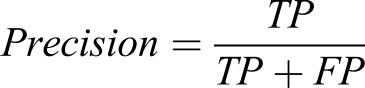
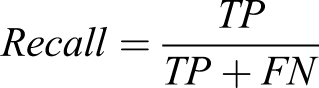
Two PEMs were used to determine the ANN performance for each of the experimental conditions. One of the PEMs used was the f1-score (Equation (1)), which is a measure of the harmonic mean between precision and recall. The precision-recall curve is a widely used PEM across machine learning literature⁵⁸

f 1 = \frac{2 (R e c a l l * P r e c i s i o n)}{R e c a l l + P r e c i s i o n}

(1)

where

P r e c i s i o n = \frac{T P}{T P + F P}

R e c a l l = \frac{T P}{T P + F N}

The second PEM used was the Area Under the Receiver Operating Characteristic Curve (ROC-AUC) (Equation (2)), which has been shown to be the more desired option when dealing with medical datasets.⁵⁹ The ROC is a curve which plots the true positive rate along the y-axis and the false positive rate along the x-axis (Equation (2) and (3)). The AUC is calculated as the area under the plotted ROC curve and provides a measure of success for each ROC plot and therefore allows for a comparison of the ROC plots across different conditions. ROC also introduces metric coverage of specificity and sensitivity⁶⁰

T P R (S e n s i t i v i t y) = \frac{T P}{T P + F N}

(2)

F P R (1 - S p e c i f i c i t y) = \frac{F P}{F P + T N}

(3)

Sample size

Sample sizes were computed to determine the number of times each method in each experimental condition was run, providing us with multiple results of the ANN system performance evaluation to act as a group of results for statistical comparisons. The standard error of mean (SEM) was calculated between the values obtained from the results of the PEM for each run of the experiment. Here, the SEM was calculated between 3 and 73 samples to derive a sufficient sample size, as portrayed in Figure 4. The electroencephalography (EEG) Eye State and the Cardiotocography datasets display the least fluctuations in SEM from sample size 3. Additionally, all dataset SEMs reached a plateau at around sample size 50. This informs us that each method should be run 50 times to obtain 50 values of the f1-score and ROC-AUC, while accounting for SEM within the sample prior to statistical analysis.

Figure 4.

Relationship between sample size and SEM. Graph demonstrates the change in SEM over increasing sample sizes. Note: SEM: standard error of mean.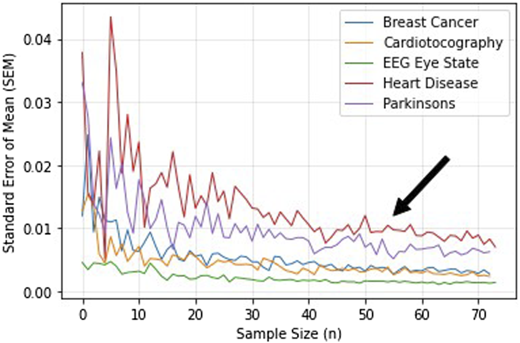

Statistical analysis

Firstly, to decide which test to use between PEMs from each of the methods depended on the distribution of the results. The Kolmogorov–Smirnov test for normality⁶¹ was conducted to extract the p-values indicating a normal or non-normal distribution for the PEM results of each condition. The findings showed a mixture of both normally (p $>$ 0.05) and non-normally (p $<$ 0.05) distributed data, indicating a non-parametric approach for testing between the re-sampling conditions.

Accordingly, the non-parametric Wilcoxon signed-rank test⁶² for testing between two groups was used between re-sampling methods within the under-sampling and over-sampling conditions. The non-parametric Friedman test⁶³ for testing between more than 2 groups was used for the combi-sampling condition. Finally, the Wilcoxon signed-rank test was also used to compare each condition in combi-sampling, over-sampling and under-sampling to the control.

Experimental results

Under-sampling and over-sampling results were determined from the direct significance testing between the methods within each re-sampling condition, that is, between SMOTE and ADASYN in over-sampling. Combi-sampling, on the other hand, utilized group comparisons for significance testing, which can be described in two measures of analysis. The first measure was to test for a significant difference amongst the convergence points within each re-sampling method. For example, we tested for whether there was a significant difference when using convergence points 1, 2, 3, 4 or 5 within the ADASYN-CC re-sampling method. The second measure of testing was across the re-sampling methods within each convergence point. For example, whether there was a significant difference between the ADASYN-CC, ADASYN-NM, SMOTE-CC, SMOTE-NM or RANDOM-RANDOM re-sampling methods with convergence point 1. Statistically significant differences between methods were defined as p <

α

, where α = 0.05 for under-sampling, over-sampling and control comparative analysis. Critical level α for combi-sampling multiple comparisons tests was adjusted to 2.5 × 10⁻³ per dataset using Bonferroni correction. Each dataset has corresponding tabulated results for the optimal strategy within re-sampling conditions (Tables 3–7), where asterisk-marked cells indicate a significant p-value. Comparative control analysis p-values are also accompanied with an indication of whether the control condition outperformed the re-sampling methods, shown by (−) and (+), favouring the control condition or re-sampling method, respectively.

Table 3.

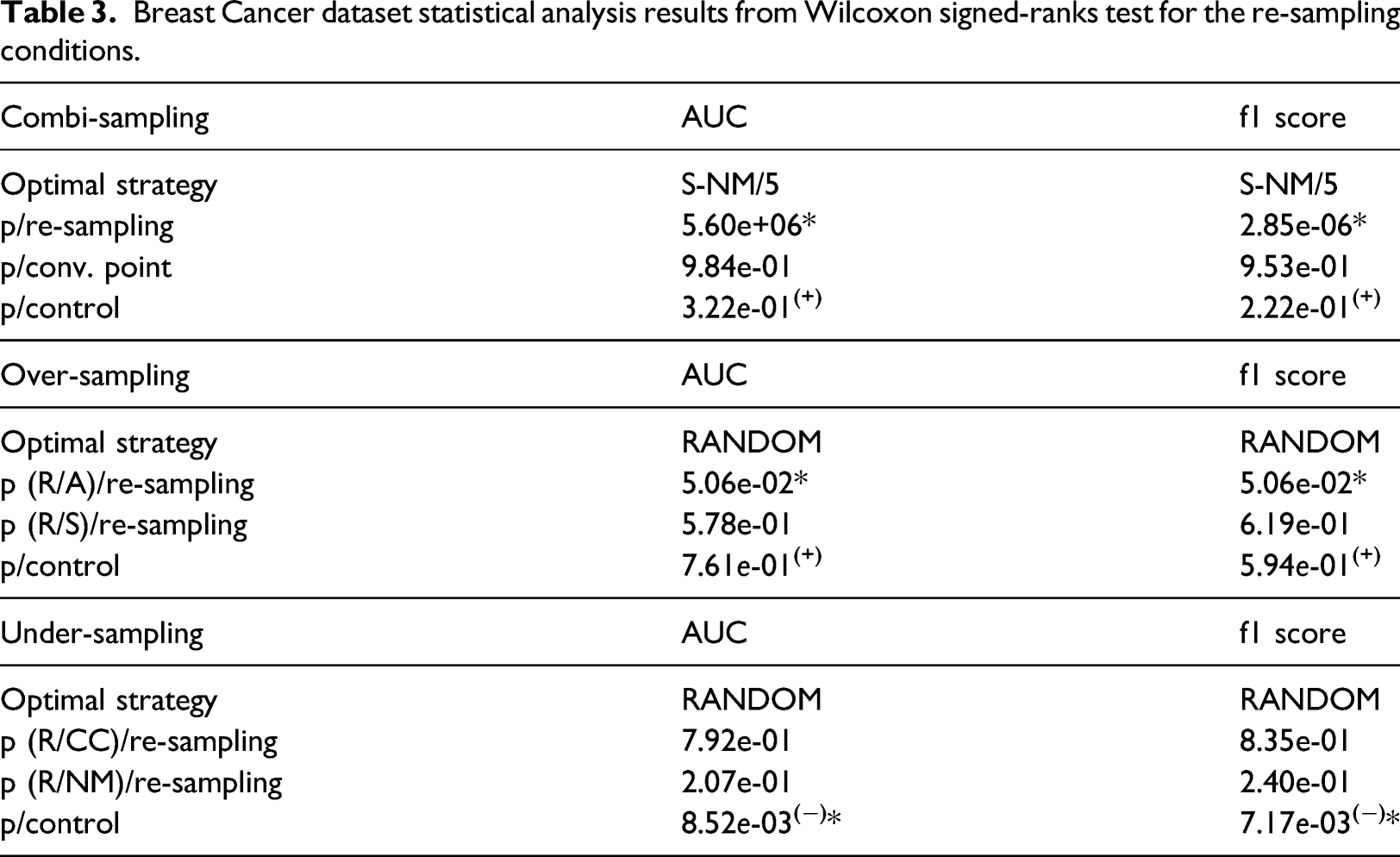
Breast Cancer dataset statistical analysis results from Wilcoxon signed-ranks test for the re-sampling conditions.

Combi-sampling	AUC	f1 score
Optimal strategy	S-NM/5	S-NM/5
p/re-sampling	5.60e+06*	2.85e-06*
p/conv. point	9.84e-01	9.53e-01
p/control	3.22e-01⁽⁺⁾	2.22e-01⁽⁺⁾
Over-sampling	AUC	f1 score
Optimal strategy	RANDOM	RANDOM
p (R/A)/re-sampling	5.06e-02*	5.06e-02*
p (R/S)/re-sampling	5.78e-01	6.19e-01
p/control	7.61e-01⁽⁺⁾	5.94e-01⁽⁺⁾
Under-sampling	AUC	f1 score
Optimal strategy	RANDOM	RANDOM
p (R/CC)/re-sampling	7.92e-01	8.35e-01
p (R/NM)/re-sampling	2.07e-01	2.40e-01
p/control	8.52e-03⁽⁻⁾*	7.17e-03⁽⁻⁾*

Table 4.

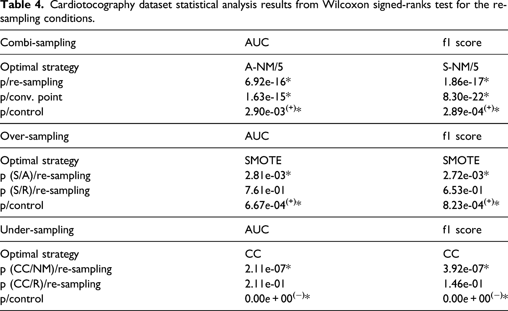
Cardiotocography dataset statistical analysis results from Wilcoxon signed-ranks test for the re-sampling conditions.

Combi-sampling	AUC	f1 score
Optimal strategy	A-NM/5	S-NM/5
p/re-sampling	6.92e-16*	1.86e-17*
p/conv. point	1.63e-15*	8.30e-22*
p/control	2.90e-03⁽⁺⁾*	2.89e-04⁽⁺⁾*
Over-sampling	AUC	f1 score
Optimal strategy	SMOTE	SMOTE
p (S/A)/re-sampling	2.81e-03*	2.72e-03*
p (S/R)/re-sampling	7.61e-01	6.53e-01
p/control	6.67e-04⁽⁺⁾*	8.23e-04⁽⁺⁾*
Under-sampling	AUC	f1 score
Optimal strategy	CC	CC
p (CC/NM)/re-sampling	2.11e-07*	3.92e-07*
p (CC/R)/re-sampling	2.11e-01	1.46e-01
p/control	0.00e + 00⁽⁻⁾*	0.00e + 00⁽⁻⁾*

Table 5.

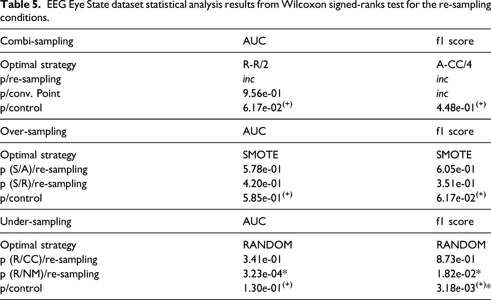
EEG Eye State dataset statistical analysis results from Wilcoxon signed-ranks test for the re-sampling conditions.

Combi-sampling	AUC	f1 score
Optimal strategy	R-R/2	A-CC/4
p/re-sampling	inc	inc
p/conv. Point	9.56e-01	inc
p/control	6.17e-02⁽⁺⁾	4.48e-01⁽⁺⁾
Over-sampling	AUC	f1 score
Optimal strategy	SMOTE	SMOTE
p (S/A)/re-sampling	5.78e-01	6.05e-01
p (S/R)/re-sampling	4.20e-01	3.51e-01
p/control	5.85e-01⁽⁺⁾	6.17e-02⁽⁺⁾
Under-sampling	AUC	f1 score
Optimal strategy	RANDOM	RANDOM
p (R/CC)/re-sampling	3.41e-01	8.73e-01
p (R/NM)/re-sampling	3.23e-04*	1.82e-02*
p/control	1.30e-01⁽⁺⁾	3.18e-03⁽⁺⁾*

Table 6.

Heart Disease dataset statistical analysis results from Wilcoxon signed-ranks test for the re-sampling conditions.

Combi-sampling	AUC	f1 score
Optimal strategy	S-NM/4	R-R/1
p/re-sampling	9.66e-04*	8.58e-04*
p/conv. point	3.22e-10*	1.00e-02
p/control	5.47e-04⁽⁺⁾*	6.31e-02⁽⁺⁾
Over-sampling	AUC	f1 score
Optimal strategy	ADASYN	ADASYN
p (A/R)/re-sampling	5.46e-01	9.80e-01
p (A/S)/re-sampling	8.21e-01	6.39e-01
p/control	4.95e-03⁽⁻⁾*	1.28e-03⁽⁻⁾*
Under-sampling	AUC	f1 score
Optimal strategy	NM	NM
p (NM/CC)/re-sampling	5.58e-04*	1.15e-04*
p (NM/R)/re-sampling	1.51e-03*	6.67e-04*
p/control	4.51e-03⁽⁻⁾*	0.00 + e00⁽⁻⁾*

Table 7.

Parkinson’s dataset statistical analysis results from Wilcoxon signed-ranks test for the re-sampling conditions.

Combi-sampling	AUC	f1 score
Optimal strategy	S-NM/4	R-R/2
p/re-sampling	9.66e-04*	8.58e-04*
p/conv. point	3.22e-10*	1.00e-02
p/control	5.47e-04⁽⁺⁾*	4.608e-03⁽⁺⁾*
Over-sampling	AUC	f1 score
Optimal strategy	ADASYN	ADASYN
p (A/R)/re-sampling	5.46e-01	9.80e-01
p (A/S)/re-sampling	8.21e-01	6.39e-01
p/control	4.95e-03⁽⁺⁾*	1.28e-03⁽⁻⁾*
Under-sampling	AUC	f1 score
Optimal strategy	NM	NM
p (NM/CC)/re-sampling	5.58e-04*	1.15e-04*
p (NM/R)/re-sampling	1.51e-03*	6.67e-04*
p/control	4.51e-03⁽⁺⁾*	0.00e + 00⁽⁻⁾*

Breast cancer

The under-sampling condition showed that random re-sampling was the best performing condition according to both the ROC-AUC and f1-score results, with significance in comparison to the control. However, neither result showed significance nor was there a significant difference between the re-sampling conditions. Furthermore, the control conditions outperformed under-sampling. Over-sampling exhibited the same findings, with random re-sampling producing the highest ROC-AUC and f1-score results; though no significant differences between methods and the control were found. For the combi-sampling condition, the Friedman test indicated that the re-sampling method of SMOTE-NM using covergence point 3 provided the best ANN performance according to the ROC-AUC and f1-score metrics. ADASYN-NM at convergence point 3 did not exhibit significant differences in comparison to the other convergence points, however, ADASYN-NM as a re-sampling method showed significant superiority in performance compared to the other combi-sampling methods. However, both performance metrics showed no significant differences with the performance of the ANN using the control data. Both optimal strategies within over-sampling and combi-sampling surpassed the control condition. The combi-sampling optimal strategies were not complimented by the optimal strategies for over-sampling and under-sampling from the results of ROC-AUC and f1-score.

Cardiotocography

The under-sampling condition showed that CC outperformed NM and random re-sampling from both the ROC-AUC and f1-score statistics, significantly so over NM. It was found, however, that the performance of CC was significantly inferior to that of the control. In the over-sampling conditions, SMOTE was the best performing re-sampling technique from both the ROC-AUC and f1-scores, and significantly different to the results of random re-sampling and ADASYN only for the f1-score results. Comparisons with the control displayed a significant superiority on ANN performance when using the f1-score metric and ROC-AUC metric. Combi-sampling found that from the ROC-AUC metric, ADASYN-NM at convergence point 5 significantly outperformed the other strategies and the control. The f1-score showed SMOTE-NM at convergence point 5 as the optimal strategy with similar performance significance. The combi-sampling optimal strategies were not complimented by the optimal strategies for over-sampling and under-sampling from the results of ROC-AUC and f1-score.

EEG eye state

For this dataset, the under-sampling condition found that the random re-sampling method outperformed both CC and NM, and significantly so for NM. Control comparative analysis resulted in greater performance of the RANDOM under-sampling method, though only significantly so from the f1-score results. In over-sampling, the ROC-AUC and f1-score results declared SMOTE as the best performing re-sampling technique, however, no significance was found between random re-sampling, ADASYN, SMOTE and the control across both PEMs.

Combi-sampling limitations were consequential with the EEG Eye State dataset, such that no convergence was obtained entirely using the convergence points 1, 2 for ADASYN-CC and convergence points 1, 2 or 3 for ADASYN-NM. The datapoints themselves could not be generated with those specific conditions. The results subsequently were extracted with the interpretation that convergence points 1, 2 and 3 provided nil performance for the ANN, resulting in an incomplete (inc) result. Thus, it was not possible to derive significance from multiple comparison analysis with missing results for the methods that failed to converge. That being said, of the remaining methods for combi-sampling, RANDOM-RANDOM at convergence point 2 and ADASYN-CC at convergence point 4 produced the highest ROC-AUC and f1-score values, respectively. It was only concluded that these results were insignificant across convergence points on the ROC-AUC space, and no significant differences were found between the optimal combi-sampling strategies and the benchmark control. In only the ROC-AUC metric did a re-sampling counterpart compliment the combi-sampling strategy, that being random under-sampling.

Heart disease

In the Heart Disease dataset, the under-sampling conditions found that the NM re-sampling condition outperformed CC and random re-sampling in both the results from the ROC-AUC and f1-score metrics. Furthermore, NM demonstrated significant differences to the control, however, the significance favours the control condition. Over-sampling found ADASYN outperforming SMOTE and random re-sampling from both PEMs, however, there was no significant difference found between all re-sampling methods, only between ADSASYN and the control. Similarly to under-sampling, the control condition produced higher ROC-AUC and f1-scores compared to re-sampling. Within combi-sampling, ROC-AUC results demonstrate an optimal re-sampling strategy of SMOTE-NM at convergence point 4. This strategy exhibits significant superiority compared to the remainder of the combi-sampling methods, convergence points and the control. The results from f1-score, on the other hand, show RANDOM-RANDOM at convergence point 1 producing the best ANN performance. This finding shows significance at only the re-sampling method level, with no significance observed between the convergence points and the control. In only the ROC-AUC metric did a re-sampling counterpart compliment the combi-sampling strategy, that being NM under-sampling.

Parkinson’s

The Parkinson’s dataset showed that NM significantly outperformed CC and random re-sampling in the under-sampling condition from both ROC-AUC and f1-score metrics. However, ANN performance was succeeded by the control condition from the f1-score results. Both control comparative analyses showed significance. In over-sampling, ADASYN was the best performing re-sampling condition – also from both PEMs. However, ADASYN had no significant differences to the other re-sampling methods; though significance was found in comparison to the control. The combi-sampling conditions showed that the SMOTE-NM re-sampling condition using the convergence point 4 significantly outperformed the other re-sampling strategies and convergence points along with a significantly superior performance compared to the control from the ROC-AUC statistic. The f1-score metric showed that RANDOM-RANDOM with convergence point 2 significantly outperformed the other re-sampling strategies and a significant superior performance to the control, however, no significance between convergence points. In only the ROC-AUC metric did a re-sampling counterpart compliment the combi-sampling strategy, that being NM under-sampling.

Visual inspection

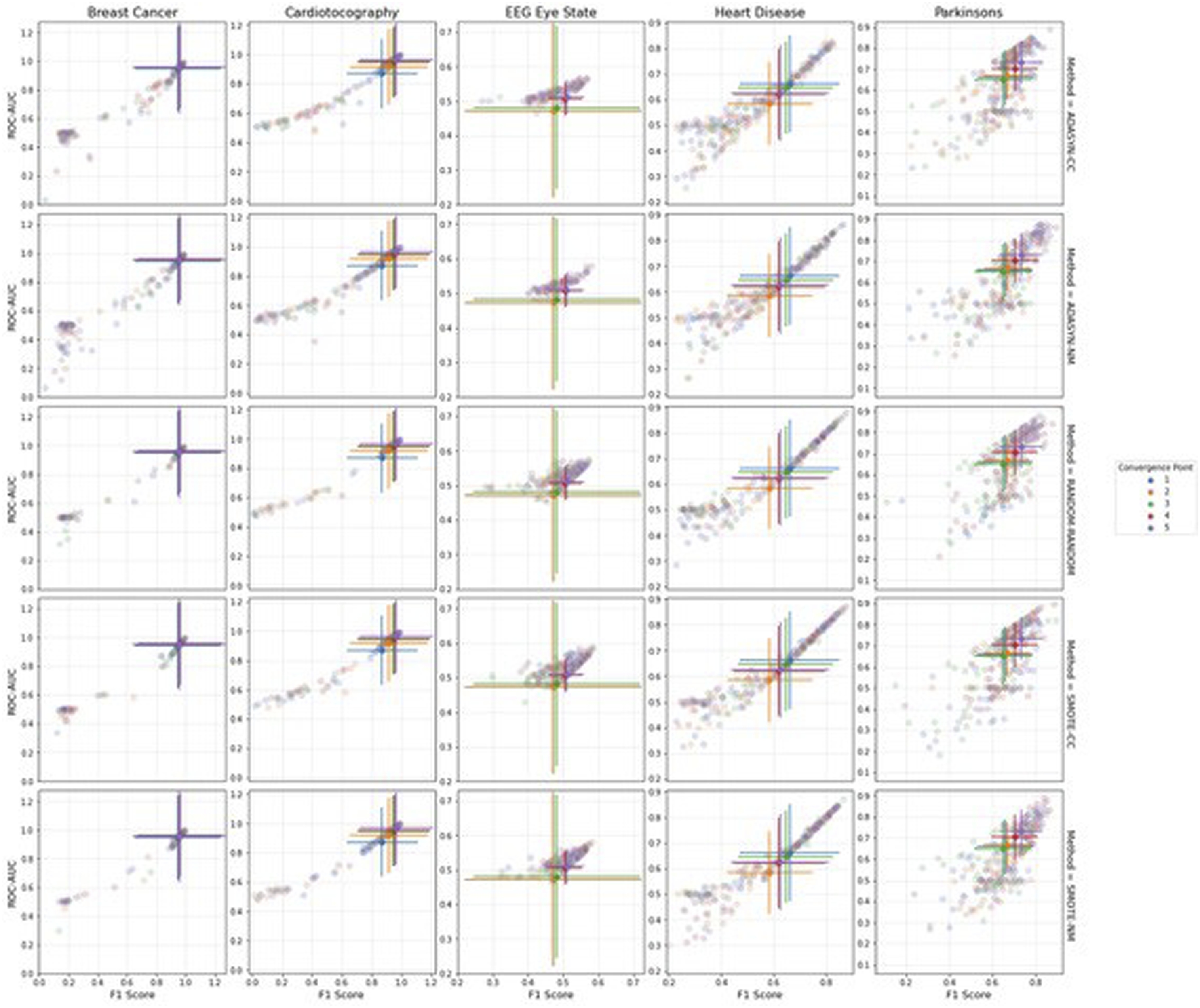
In Figures 5–7, we demonstrate the pattern of the f1-score against the ROC-AUC to observe the directional relationship between the two metrics. Error bars on the scatterplots depict the standard deviation which are centred at the median of the sample, complimenting the p-values in Tables 3–7. Difference in performance significance decreases as the error bars that represent each re-sampling method (shown in legend) come closer to overlapping completely. However, the more discrete the error bars, the clearer the ANN performance distinction. This can be observed with the Heart Disease dataset in the under- and over-sampling conditions (Figure 5, where it is illustrated that the error bars are the most visually discrete. This is complimented by Table 6, where the optimal strategies are coherent between the f1-score and ROC-AUC.

Figure 5.

Scatterplots visualizing the range of Artificial neural networks performance from the ROC-AUC and f1-scores for (a) under-sampling, and (b) over-sampling conditions, colour coded by re-sampling method. Error bars represent the standard deviation, centred at the median of the sample.

Figure 6.

Scatterplots visualizing the range of Artificial neural networks performance from the ROC-AUC and f1-scores for the combi-sampling condition, colour coded by re-sampling method. Each row corresponds to a convergence point. Error bars represent the standard deviation, centred at the median of the sample.

Figure 7.

Scatterplots visualizing the range of Artificial neural networks performance from the ROC-AUC and f1-scores for the combi-sampling condition, colour coded by convergence point. Each row corresponds to a re-sampling method. Error bars represent the standard deviation, centred at the median of the sample.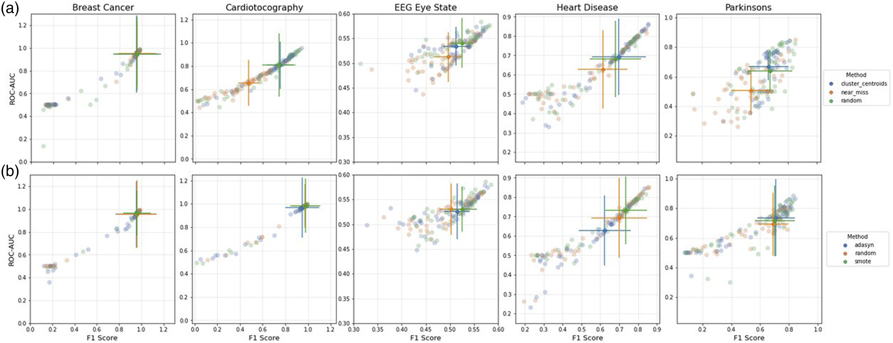

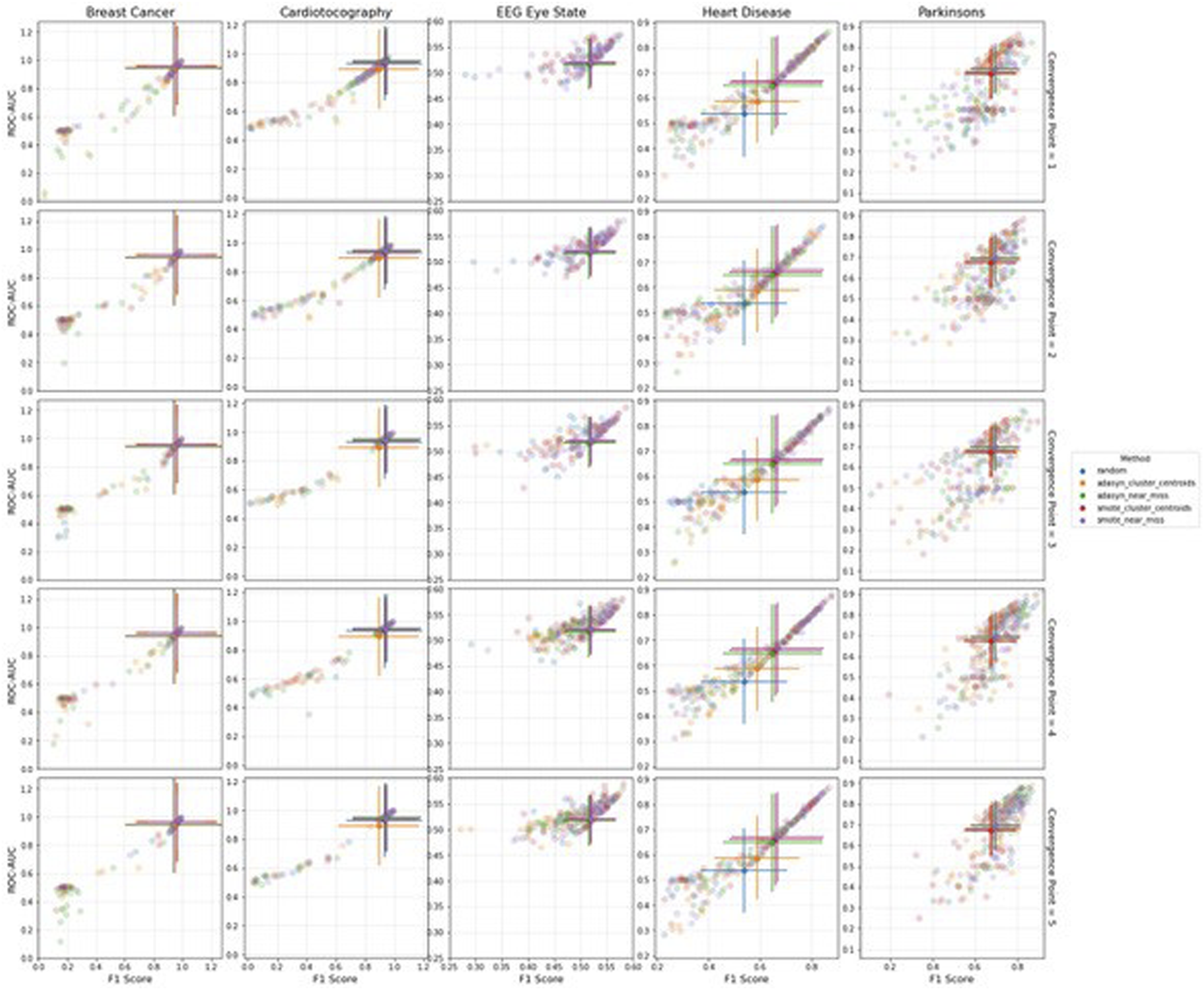
Across all re-sampling conditions for the Breast Cancer and Cardiotocography datasets, and the under-sampling plot for the Parkinson’s dataset, the scatterplots display a gradual correlation which shows that the values of ROC-AUC seldom drop below 0.4 while the f1-scores approach 0. The scatterplot pattern deviates from the 45° diagonal (which indicates equal f1-score and ROC-AUC values). This demonstrates that as the ROC-AUC values approach matching amounts of true negatives and true positives, the relevance of the predictions, depicted by the f1-score, swiftly approach zero; due to the proportion true positive results to all positive results.

The Heart Disease dataset exhibits the most coherence to the diagonal across all re-sampling conditions, suggesting that the components of this dataset is often less biased towards either of the PEMs. The benefits for datasets that exhibit this behaviour can stipulate that where high values of the f1-score are produced, they are likely to be accompanied with a high value of the ROC-AUC. While the Parkinson’s and EEG Eye State datasets also cohere to the diagonal, the elements are considerably more dispersed compared to the Heart Disease dataset. The EEG Eye State dataset scatterplot form a tighter cluster; however, it should be taken into account the lack of results from computational limitations for the convergence points using ADASYN for over-sampling. In Figure 7, this complication can be seen where the error bars are blown out of proportion for the convergence points which failed to generate datapoints and therefore provided nil performance for the ANN. On the other hand, in the over-sampling and under-sampling plots for the EEG Eye State dataset, the performance of the ANN increases in such a way that the f1-score and ROC-AUC values close in on the diagonal. However, as performance decreases, there is less of a coherence with the diagonal – decreasing more rapidly on the f1-score axis than the ROC-AUC.

Discussion

The statistical analysis methods used, multiple comparisons (Friedman), Wilcoxon Signed-Ranks and correction using Bonferroni tests, were specifically chosen to account for the stochastic nature of the algorithms employed in the re-sampling conditions. This demonstrated a consideration of the significance of the results upon interpretation.

For the Heart Disease, Breast Cancer and Parkinson’s datasets, it is important to consider dataset variability and size. These datasets are markedly smaller in comparison to the EEG Eye State and Cardiotocography datasets, and by nature will possess a decreased variability in data (and increase in variance)⁶⁴ causing them to be prone to over-fitting. In such a case, the ANN would memorize values rather than patterns.⁶⁵ Therefore, when analysing the results, larger datasets would be required should the purpose of the ANN be applied to new data. Another important consideration is the distance between minority and majority classes. For example, for the Heart Disease dataset, the difference between minority and majority classes was only 23 instances. It was expected that in such datasets the difference in performance between convergence points be insignificant, due to such a small difference between minority and majority classes. Hence, combi-sampling would not be the most suitable re-sampling technique under the conditions of small datasets and small minority-majority distances.

The minority-majority ratios to the nearest integer for each dataset are as follows: Breast Cancer 1:2, Cardiotocography 1:8, EEG Eye State 3:4, Heart Disease 5:6 and Parkinson’s 1:3. The ratio within datasets between minority and majority classes did not show a clear link with the PEMs. For instance, the Cardiotocography and Parkinson’s datasets exhibit the highest ratios and both showed significant differences to the control in ANN performance after re-sampling under all conditions. Which concurs with previous research that has shown that when the ratio between minority and majority classes are high, this deteriorates the results from the PEMs.^66,67 On the other hand, the EEG dataset by comparison had a lower ratio whilst also performing significantly better than the control after each re-sampling condition, supported by research finding that when there is a strong imbalance, standard classifiers would produce sufficiently accurate performance.⁶⁸ The remaining datasets, Heart Disease and Breast Cancer, had lower ratios in comparison to Cardiotocography and Parkinson’s. However, the Heart Disease dataset did not produce significant differences to the control performance across all re-sampling conditions. These results are in line with existing literature which state that class imbalance ratios may not necessarily be the only hindrance on ANN performance for datasets with imbalanced classes.⁶⁸

There were difficulties encountered during the implementation of the ADASYN over-sampling algorithm into combi-sampling for the larger-scale datasets in this study. The decision function of the ADASYN algorithm generates new datapoints by focussing on the boundaries of the feature space⁵⁰ with the aim of removing the skew of data. What was observed from ADASYN was that there were little to no datapoints being generated when the convergence points were closer to the minority class, despite being capable of successfully over-sampling the minority class on its own. This suggested that it was unsuitable for ADASYN to be implemented into a combi-sampling approach when dealing with larger datasets, specifically to re-sample a minority class to a size near the value of its own.

In each dataset, the combi-sampling condition produced significantly higher ANN performance than the control. However, f1-scores favoured random re-sampling for the Heart Disease and Parkinson’s datasets; while the ROC-AUC does the same with the EEG Eye State dataset. For under-sampling only, the EEG Eye State dataset also favours random re-sampling significantly so over NM and the control for both PEMs. The Breast Cancer did not comply with either of the advanced re-sampling methods for both under- and over-sampling, rather performing best with random re-sampling. Proving a significant superiority over ADASYN and the control in over-sampling, it contrarily exhibits significantly poorer performance compared to the control in under-sampling. These findings deduce that there is an incompatibility between these datasets and the re-sampling algorithms; whereby the chance results serve as an indication towards alternative re-sampling methods, requiring a more extensive review between a greater range of re-sampling algorithms on the specific dataset to shed light behind the reasoning for sub-optimal performance.⁶⁹

Optimal method consistency between combi-sampling and over-/under-sampling conditions were found within under-sampling and results of the ROC-AUC only. This consistency occurred for the EEG Eye State, Heart Disease and Parkinson’s datasets, while the remaining datasets showed no such consistencies. Furthermore, between PEMs, only the Breast Cancer dataset showed consistency for the optimal combi-sampling strategy – inclusive of re-sampling and convergence point methods. The Cardiotocography dataset showed consistency between the PEMs in the under-sampling counterpart and convergence point, however, not for the over-sampling counterpart. The remaining datasets conveyed no distinct consistencies in the optimal strategies for the combi-sampling condition between f1-scores and ROC-AUC. On the other hand, over-sampling and under-sampling demonstrated consistency in re-sampling method across PEMs.PEMs are derived from different statistical powers of the data; where PEMs display discordant results for the same classifier on the same dataset, this is indicative of an aspect of the dataset which lacks in quality and/or the classifier is not sufficiently built for the dataset. As mentioned in Experimental Protocol, using more than one PEM to measure performance can help provide a more comprehensive view of the ANN. Particularly in this study, as four of the main metrics (precision and recall for the f1-score,⁷⁰ sensitivity and specificity for the ROC-AUC⁶⁰) are utilized. Consider a confusion matrix which illustrates true positives, false positives, true negatives and false negatives. Sensitivity and recall both measure how well the positives are predicted by a classifier. As such, the value of sensitivity or recall could be increased during training by simply maximizing the predictions for positive. This is the same with specificity, which measures how well false positives are predicted, can be maximized by consistently returning the predictions for negatives. Precision measures the relevance of the predicted result, that is, correctly labelled predictions. If only one prediction was returned that was a sure-fire correct label, this would return a good precision value. In light of this, it would be useful to carefully inspect the dataset when building the re-sampling and classifier pipeline so to minimize any bias contributing to any one performance metric due to weaknesses that exist in the dataset. For the purposes of this experiment, the classifier model was kept consistent for each condition that was implemented. This could explain the differences in the report for optimal re-sampling technique as the classifier could be more appropriately suited for one dataset over another.

For example, the f1-score and ROC-AUC metrics reported conflicting results in the over-sampling counterpart of the combi-sampling condition for the Cardiotocography dataset. Without the presence of the f1-score, it would have been deduced that ADASYN was the most suitable given the p-value generated in comparison to the other re-sampling techniques and the control. However, results from the f1-score analysis suggest that in fact SMOTE was most suitable for the over-sampling counterpart – in coherence with the results from the over-sampling condition for both f1-score and ROC-AUC. This indicates that certain factors of each over-sampling technique imposed onto the dataset in combi-sampling were favoured by the individual PEMs.⁷¹ From a standpoint of dataset quality,^72,73 because the under-sampling and convergence points are consistent between PEMs, it could be interpreted that there are issues rooted at the datapoint generation of the minority class. In a state of uncertainty such as this, further investigation is recommended; for example, testing between each re-sampling conditions would detail whether ADASYN-NM/5 significantly outperforms over-sampling only with SMOTE (where SMOTE is the optimal strategy concerning both PEMs). If the outcome turns out to be false, this suggests that ADASYN is in fact reducing the ANN performance in the space of precision and recall – which is obscured by focussing only on sensitivity and specificity with ROC-AUC.

In the results for Heart Disease and Parkinson’s datasets, it can be observed that ROC-AUC comparative analysis in combi-sampling shows a significantly superior performance of SMOTE-NM to the other re-sampling techniques and the control. Contrarily, in the under-sampling condition of the same dataset, NM was superseded by the control condition. This finding argues that for under-sampling the Heart Disease and Parkinson’s majority classes, NM would be the best approach where random re-sampling and CC are the other contenders. However, the minority class size was not sufficient to train the ANN and produce a performance level that is greater than chance. The discordance of ANN performance leads a notion that in the strictest sense of re-sampling to either the minority or majority class sizes, over-sampling yields a greater likelihood of good performance³⁵ – though in spite of this, it is indeed possible to generate a class size smaller than the majority and generate significantly superior results to the control.

A final factor of the experiments concerns the consistency between convergence points within the combi-sampling condition. Out of the 10 findings, 7 optimal strategies possess a convergence point of 4 or above. The higher levels of convergence points elevate the performance of the ANN significantly above the control across all datasets, and produce a significant improvement above the other convergence points for all corresponding datasets except for EEG Eye State where this finding was inconclusive. In the Parkinson’s dataset, SMOTE-NM at convergence point 4 outperformed all other combi-sampling methods and the control. However, the corresponding over-sampling only methods were insignificant while the under-sampling methods were. This shows a boost from both the under-sampling counterpart and convergence point, that are able to generate datapoints which carry far more relevant information than over-sampling alone, albeit the class size must be close the majority class. This concept is also reflected in the Parkinson’s dataset, where neither the over-sampling or under-sampling conditions were able to succeed the ANN performance above the control; though the combination of the re-sampling methods generated new datapoints that significantly better the ANN performance at a convergence point close to the majority class size. Of those that had an optimal convergence point below 4, they were all accompanied by random re-sampling for both the under- and over-sampling counterparts. These results hone in on the importance of class size; suggesting that while indeed re-sampling improves the performance of the ANN above the control, the re-sampling algorithms aren’t able to produce a higher performance above chance regardless of the class size so long as the size is between the minority and majority classes. In fact, this statement is supported by the p-values from the Friedman multiple comparisons analysis, which states that there are no significant differences in the performance of the ANN across convergence points for all datasets that exhibit an optimal strategy of RANDOM-RANDOM.

These discrepancies across re-sampling strategies, convergence points and PEMs are directly related to the no-free-lunch theorem (NFL)⁷⁴ and the bias-variance trade-off. The NFL, in machine learning terms, states that there are no universal solutions and declare that all techniques and algorithms can be deemed as good as each other if no assumptions are placed on the dataset at hand.⁷⁵ Furthermore, studies have shown that the NFL theorem applies especially for supervised learning models.⁷⁶ The NFL has been widely implemented by machine learning literature,⁷⁷ providing precautions to building machine learning models. The theorem proves that there is no feasible way for an algorithm or model to succeed equally at two different problems. It is therefore not illogical for the dataset or pre-processing of the dataset to hold an equal, if not greater, importance to the algorithm employed.⁷⁷ The bias-variance trade-off corresponds to the trade-off between under-fitting (high bias) and over-fitting (high variance).⁷⁸ Imbalanced datasets have skews, and the way in which the balance of this trade-off is restored depends not only on the original skew, but also on how well the dataset responds to the methods that attempt to restore it. For example, large datasets with a very clear decision boundary may be susceptible to over-fitting if too powerful a technique is employed to reduce the bias. The bias-variance trade-off ties into the NFL theorem whereby the dataset steers the approach taken to deal with the problem.

Conclusion

The purpose of re-sampling is to generate equal class sizes from datasets which have events pertaining to one classification that exceed the instances of the other event(s). By customizing pre-processing stages, such as re-sampling manipulation on the data, and taking into consideration the distinctive complexity of its features; future predictive models could be improved given that re-sampling is a necessary process to the build of that AI system. The main objective of this study was to demonstrate how it can be crucial to take different approaches to re-sampling problems, and for users in industry to have clarity on this matter. The results of this experiment show that both algorithms and performance evaluation metrics can favour a specific type of dataset over another, despite consisting of data from the same industry. The distinctions are not only between the overall re-sampling technique across the different datasets (combi-sampling, over-sampling and under-sampling) but also significantly distinct differences within the re-sampling techniques themselves.

There have been a number of limitations to this study, which paves way for future studies relating to this research topic. For example, the ANN structure and parameter configuration was kept constant here as to minimize contributing factors. However, building the ANN to perform optimally specific to each dataset might shed light on whether the performances would still differ across re-sampling techniques. Alternatively, several large datasets could be used as to eliminate dataset quantity as a contributing factor to the performance of the ANN. Additionally, different machine learning paradigms within supervised, unsupervised, semi-supervised or reinforced learning suitable for classification problems could provide other possibilities for design protocol or experimental results. Furthermore, another approach is to implement different re-sampling strategies. For example, Tomek Links⁷⁹ or Edited Nearest Neighbours⁸⁰ are alternate options for under-sampling. As this applies also to over-sampling, by extension combination of techniques for combi-sampling. One final suggestion for further work is the comparison of the re-sampling conditions within each dataset. Currently, a number of comparative literatures explores classification algorithms,^81–83 re-sampling techniques^84–86 or model configurations^87,88 can be found. Though more re-sampling comparative papers which include the novel method of combi-sampling is required.

AI is an incredibly useful tool in solving industrial problems. It must, however, be delivered with stringent guidelines and caution to the level of responsibility that is assigned to the automation. It has been previously suggested that ANNs should primarily be used as a proof-of-concept product rather than a standalone predictive model in the healthcare industry.⁸⁹ While ANNs have had significant impact with data analytics, there is a lack of transparency for the ability to explain the decision-making process and arising to issues with interpretability.^4,90 These challenges hinder the widespread adoption of AI in healthcare. Data-driven models begin to tackle these challenges by gearing the predictive model to address the characteristics of the dataset in hand, rather than implementing a previously generated and potentially outdated or irrelevant model. Furthermore, data-driven models leverage having a clear identification of output labels from experts in the field⁹¹ to support the interpretation of the model outputs. Re-sampling techniques alleviate the reduction in model performance when datasets are irregular; the aim of this paper is to demonstrate that, similarly to demand for transparency of the model itself, the re-sampling pipeline of the data should also factor into the data-driven approach. Understanding that different re-sampling techniques produce different results across datasets is a part of improving the clarity of the underlying rationale of the overall AI approach in healthcare.⁹² It is vital that the message is conveyed for responsible use of AI within the industry network in order to maintain integrity for technology and safety for the clients and users. This paper demonstrates the inherent potential of inconsistencies that can arise with the assumptions for over-generalized use of AI systems.

Footnotes

Declaration of conflicting interests

The author(s) declared no potential conflicts of interest with respect to the research, authorship, and/or publication of this article.

Funding

The author(s) disclosed receipt of the following financial support for the research, authorship, and/or publication of this article: Marcia Saul received financial support for the publication of this article through the Open Access Fund from Bournemouth University.

Author note

Python code for all re-sampling experiments and statistical analysis available on request.

ORCID iD

Marcia Saul

References

Esteva

Kuprel

Novoa

, et al. Dermatologist-level classification of skin cancer with deep neural networks. Nature 2017; 542(7639): 115–118.

Zhou

Troyanskaya

. Predicting effects of noncoding variants with deep learning-based sequence model. Nat Methods 2015; 12(10): 931–934.

Sordo

. Introduction to Neural Networks in Healthcare. Open Clinical: Knowledge Management for Medical Care, 2002.

Shahid

Rappon

Berta

. Applications of artificial neural networks in health care organizational decision-making: a scoping review. PloS One 2019; 14(2): e0212356.

Schocken

Ariav

. Neural Networks for Decision Support Systems: Problems and Opportunities. New York: New York University: Center for Research on Information Systems, Stern School of Business, 1991.

Moghimi

Wickramasinghe

. Artificial neural network excellence to facilitate lean thinking adoption in healthcare contexts. In: Lean Thinking for Healthcare. New York: Springer; 2014, pp. 13–27.

Bajo

de Paz

, et al. Integrating case-based planning and rptw neural networks to construct an intelligent environment for health care. Expert Syst Appl 2009; 36(3): 5844–5858.

Japkowicz

Stephen

. The class imbalance problem: a systematic study1. Intell Data Anal 2002; 6(5): 429–449. DOI: 10.3233/ida-2002-6504.

Estabrooks

. A Combination Scheme for Inductive Learning from Imbalanced Data Sets, PhD Thesis. DalTech, 2000.

10.

Estabrooks

Japkowicz

. A multiple resampling method for learning from imbalanced data sets. Comput Intell 2004; 20(1): 18–36.

11.

Haixiang

Yijing

Shang

, et al. Learning from class-imbalanced data: review of methods and applications. Expert Syst Appl 2017; 73: 220–239.

12.

Barbieri

Chawla

Zaccagni

, et al. Predicting cardiovascular risk in athletes: resampling improves classification performance. Int J Environ Res Public Health 2020; 17(21): 7923.

13.

Huang

Chan

T-M

Dong

. Mace prediction of acute coronary syndrome via boosted resampling classification using electronic medical records. J Biomed Inform 2017; 66: 161–170.

14.

Dubey

Zhou

Wang

, et al. Analysis of sampling techniques for imbalanced data: an n=648 ADNI study. NeuroImage 2014; 87: 220–241.

15.

Lee

. Resampling methods improve the predictive power of modeling in class-imbalanced datasets. Int J Environment Res Public Health 2014; 11(9): 9776–9789.

16.

Allen

. Photoplethysmography and its application in clinical physiological measurement. Physiol Meas 2007; 28(3): R1–R39. DOI: 10.1088/0967-3334/28/3/r01.

17.

Kim

Yoo

. Motion artifact reduction in photoplethysmography using independent component analysis. IEEE Trans Biomed Eng 2006; 53(3): 566–568. DOI: 10.1109/tbme.2005.869784.

18.

Sun

Papin

Azorin-Peris

, et al. Use of ambient light in remote photoplethysmographic systems: comparison between a high-performance camera and a low-cost webcam. J Biomed Opt 2012; 17(3): 037005. DOI: 10.1117/1.jbo.17.3.037005.

19.

Leonard

Clifton

Addison

, et al. An automated algorithm for determining respiratory rate by photoplethysmogram in children. Acta Paediatr 2006; 95(9): 1124–1128. DOI: 10.1080/08035250600612280.

20.

Segev

. Integrating computer vision with web-based knowledge for medical diagnostic assistance. Expert Syst 2010; 27(4): 247–258. DOI: 10.1111/j.1468-0394.2010.00520.x.

21.

Zhu

Zhang

Hirdes

, et al. Using machine learning algorithms to guide rehabilitation planning for home care clients. BMC Med Inform Decis Making 2007; 7(1). DOI: 10.1186/1472-6947-7-41.

22.

Barbash

Glied

. New technology and health care costs - the case of robot-assisted surgery. New Engl J Med 2010; 363(8): 701–704. DOI: 10.1056/nejmp1006602.

23.

Campbell

. The Robot Will See You Now: How Ai Could Revolutionise Nhs. The Guardian, 2018.

24.

Team

. Ai and Healthcare: A Giant Opportunity. Forbes, 2019. URL, https://www.forbes.com/sites/insights-intelai/2019/02/11/ai-and-healthcare-a-giant-opportunity/

25.

Kaur

Pannu

Malhi

. A systematic review on imbalanced data challenges in machine learning: applications and solutions. ACM Comput Surv (Csur) 2019; 52(4): 1–36.

26.

Rao

Makkithaya

. Learning from a class imbalanced public health dataset: a cost-based comparison of classifier performance. Int J Electr Comp Eng (IJECE) 2017; 7(4): 2215.

27.

Abd Elrahman

Abraham

. A review of class imbalance problem. J Netw Innovative Comput 2013; 1(2013): 332–340.

28.

Thai-Nghe

Gantner

Schmidt-Thieme

. Cost-sensitive learning methods for imbalanced data. In: The 2010 International joint conference on neural networks (IJCNN), Barcelona, Spain, 18–23 July 2010. IEEE, pp. 1–8.

29.

Liu

. A comparative study on rough set based class imbalance learning. Knowl Based Syst 2008; 21(8): 753–763.

30.

Uci Machine Learning Repository : https://archive.ics.uci.edu/ml/index.php, 2018. URL https://archive.ics.uci.edu/ml/index.php.

31.

Eddy

. Large data sets in statistical computing. Int Encyclopedia Soc Behav Sci 2001; 8382–8386. DOI: 10.1016/b0-08-043076-7/00449-6.

32.

Horton

Kleinman

. Much ado about nothing. Am Statistic 2007; 61(1): 79–90.

33.

Allison

. Missing Data. Thousand Oaks, CA: Sage, 2010.

34.

Cheema

. Some general guidelines for choosing missing data handling methods in educational research. J Mod Appl Stat Methods 2014; 13(2): 3.

35.

Saul

Rostami

. A comparison of re-sampling techniques for pattern classification in imbalanced data-sets. In: Advances in Intelligent Systems and Computing. Cham: Springer, 2018, pp. 240–251. DOI: 10.1007/978-3-319-97982-3˙20.

36.

Hornik

Stinchcombe

White

. Multilayer feedforward networks are universal approximators. Neural Networks 1989; 2(5): 359–366.

37.

Cybenko

. Approximation by superpositions of a sigmoidal function. Math Control Signals, Syst 1989; 2(4): 303–314.

38.

Janocha

Czarnecki

. On loss functions for deep neural networks in classification. Schedae Informaticae 2017; 1/2016. DOI: 10.4467/20838476si.16.004.6185, URL: https://arxiv.org/pdf/1702.05659.pdf

39.

Bottou

Curtis

Nocedal

. Optimization methods for large-scale machine learning. Siam Rev 2018; 60(2): 223–311.

40.

Goodfellow

Bengio

Courville

. Deep Learning. Cambridge, MA: The Mit Press, 2017.

41.

Duchi

Hazan

Singer

. Adaptive subgradient methods for online learning and stochastic optimization. J Machine Learn Res 2011; 12(Jul): 2121–2159.

42.

Kaya

Kayci

Tekin

. A computer vision system for the automatic identification of butterfly species via gabor-filter-based texture features and extreme learning machine: Gf+ elm. TEM J 2013; 2(1): 13–20.

43.

Rong

Ong

Tan

, et al. A fast pruned-extreme learning machine for classification problem. Neurocomputing 2008; 72(1–3): 359–366.

44.

Olson

Moore

. Tpot: a tree-based pipeline optimization tool for automating machine learning. In: Workshop on automatic machine learning, New York, NY, USA, 24 Jun 2016. PMLR, pp. 66–74.

45.

Costa

Lorena

Carvalho

, et al. A review of performance evaluation measures for hierarchical classifiers. In: Evaluation Methods for machine Learning II: papers from the AAAI-2007 Workshop, San Francisco, California, USA, February 4-9 2017, pp. 1–6.

46.

Ferri

Hernández-Orallo

Modroiu

. An experimental comparison of performance measures for classification. Pattern Recognit Lett 2009; 30(1): 27–38. DOI: 10.1016/j.patrec.2008.08.010.

47.

Sokolova

Lapalme

. A systematic analysis of performance measures for classification tasks. Inf Process Manag 2009; 45(4): 427–437. DOI: 10.1016/j.ipm.2009.03.002, URL: https://www.sciencedirect.com/science/article/pii/S0306457309000259.

48.

Under-sampling - imbalanced learn 0.5.0 documentation, 2010. URL https://imbalanced-learn.readthedocs.io/en/stable/under˙sampling.html

49.

Chawla

Bowyer

Hall

, et al. Smote: synthetic minority over-sampling technique. J Artificial Intell Res 2002; 16: 321–357.

50.

Bai

Garcia

, et al. Adasyn: adaptive synthetic sampling approach for imbalanced learning. In: 2008 IEEE International Joint Conference on Neural Networks (IEEE World Congress on Computational Intelligence), Hong Kong, 1–8 June 2008. IEEE, pp. 1322–1328.

51.

Over-sampling - imbalanced learn 0.5.0 documentation, 2009. URL https://imbalanced-learn.readthedocs.io/en/stable/over˙sampling.html.

52.

Hahnloser

RHR

Sarpeshkar

Mahowald

, et al. Digital selection and analogue amplification coexist in a cortex-inspired silicon circuit. Nature 2000; 405(6789): 947–951.

53.

Sharma

. Activation functions in neural networks, 2017. URL: https://towardsdatascience.com/activation-functions-neural-networks-1cbd9f8d91d6.

54.

Han

Moraga

. The influence of the sigmoid function parameters on the speed of backpropagation learning. In: International Workshop on Artificial Neural Networks. Berlin, Heidelber: Springer, 1995, pp. 195–201.

55.

Shin

H-C

Orton

Collins

, et al. Organ detection using deep learning. In: Medical Image Recognition, Segmentation and Parsing. Amsterdam: Academic Press, 2016, pp. 123–153. DOI: 10.1016/b978-0-12-802581-9.00007-x.

56.

Hinton

Krizhevsky

Sutskever

, et al. System and method for addressing overfitting in a neural network. US Patent 9,406,017, 2016.

57.

Yao

Rosasco

Caponnetto

. On early stopping in gradient descent learning. Construct Approx 2007; 26(2): 289–315.

58.

Saito

Rehmsmeier

. The precision-recall plot is more informative than the roc plot when evaluating binary classifiers on imbalanced datasets. PloS One 2015; 10(3): e0118432.

59.

Jin Huang

Ling

. Using auc and accuracy in evaluating learning algorithms. IEEE Trans Knowledge Data Eng 2005; 17(3): 299–310.

60.

Fawcett

. An introduction to roc analysis. Pattern Recognit Lett 2006; 27(8): 861–874.

61.

Massey

Jr . The kolmogorov-smirnov test for goodness of fit. J Am Statistical Assoc 1951; 46(253): 68–78.

62.

Wilcoxon

. Individual comparisons by ranking methods. In: Breakthroughs in Statistics. New York, NY: Springer; 1992, pp. 196–202.

63.

Friedman

. The use of ranks to avoid the assumption of normality implicit in the analysis of variance. J Ame Statist Associat 1937; 32(200): 675–701.

64.

Brain

Webb

. On the effect of data set size on bias and variance in classification learning. In: Proceedings of the Fourth Australian Knowledge Acquisition Workshop. University of New South Wales, 2000, pp. 117–128.

65.

Brownlee

. Better Deep Learning: Train Faster, Reduce Overfitting, and Make Better Predictions. Machine Learning Mastery, 2018.

66.

Grzymala-Busse

Stefanowski

Wilk

. A comparison of two approaches to data mining from imbalanced data. In: International Conference on Knowledge-Based and Intelligent Information and Engineering Systems. Berlin, Heidelberg: Springer, 2004, pp. 757–763.

67.

Japkowicz

Shah

. Evaluating Learning Algorithms: A Classification Perspective. Cambridge: Cambridge University Press, 2011.

68.

Napierala

Stefanowski

Types of minority class examples and their influence on learning classifiers from imbalanced data. J Intell Inf Syst 2016; 46(3): 563–597.

69.

. Survey of Resampling Techniques for Improving Classification Performance in Unbalanced Datasets. arXiv preprint arXiv:160806048 , 2016.

70.

Sasaki

. The truth of the f-measure. Teach Tutor Mater 2007; 1(5): 1–5.

71.

Fourure

Javaid

Posocco

, et al. Anomaly detection: how to artificially increase your f1-score with a biased evaluation protocol. In: Joint European Conference on Machine Learning and Knowledge Discovery in Databases. Cham: Springer, 2021, pp. 3–18.

72.

Kerr

Norris

Stockdale

. Data quality information and decision making: a healthcare case study. In: ACIS 2007 Proceedings, Toowoomba, 5–7 December 2007, p. 98.

73.

Tekieh

Raahemi

. Importance of data mining in healthcare: a survey. In: Proceedings of the 2015 IEEE/ACM International Conference on Advances in Social Networks Analysis and Mining, Paris, France, 25–28 August 2015, pp. 1057–1062.

74.

Wolpert

Macready

, et al. No free lunch theorems for optimization. IEEE Trans Evolut Comput 1997; 1(1): 67–82.

75.

Kawaguchi

Kaelbling

Bengio

. Generalization in Deep Learning. arXiv preprint arXiv:171005468 , 2017.

76.

Wolpert

. The supervised learning no-free-lunch theorems. In: Soft Computing and Industry. London: Springer; 2002, pp. 25–42.

77.

Gómez

Rojas

. An empirical overview of the no free lunch theorem and its effect on real-world machine learning classification. Neural Comput 2016; 28(1): 216–228.

78.

Geman

Bienenstock

Doursat

. Neural networks and the bias/variance dilemma. Neural Comput 1992; 4(1): 1–58.

79.

Tomek

. Two modifications of cnn. IEEE Trans Systems, Man Cybernetics 1976; 6: 769–772.

80.

Alejo

Sotoca

Valdovinos

, et al. Edited nearest neighbor rule for improving neural networks classifications. In: International Symposium on Neural Networks. Berlin, Heidelberg: Springer, 2010, pp. 303–310.

81.

Abu-Nimeh

Nappa

Wang

, et al. A comparison of machine learning techniques for phishing detection. In: Proceedings of the anti-phishing working groups 2nd annual eCrime researchers summit, Sanibel Island, Florida, USA, 4 October 2007. ACM, pp. 60–69.

82.

Kwokleung Chan

Te-Won Lee

Sample

, et al. Comparison of machine learning and traditional classifiers in glaucoma diagnosis. IEEE Trans Biomed Eng 2002; 49(9): 963–974.

83.

Forman

Cohen

. Learning from little: comparison of classifiers given little training. In: European Conference on Principles of Data Mining and Knowledge Discovery, Pisa, Italy, & September 20-24, 2004. Springer, pp. 161–172.

84.

Minaei-Bidgoli

Topchy

Punch

. A comparison of resampling methods for clustering ensembles. In: IC-AI, Las Vegas, Nevada, USA, 21–24 June 2004, pp. 939–945.

85.

Molinaro

Simon

Pfeiffer

. Prediction error estimation: a comparison of resampling methods. Bioinformatics 2005; 21(15): 3301–3307.

86.

Lasota

Telec

Trawiński

, et al. Empirical comparison of resampling methods using genetic fuzzy systems for a regression problem. In: International Conference on Intelligent Data Engineering and Automated Learning. Berlin, Heidelberg: Springer, 2011, pp. 17–24.

87.

Naghibi

Pourghasemi

. A comparative assessment between three machine learning models and their performance comparison by bivariate and multivariate statistical methods in groundwater potential mapping. Water Resource Manag 2015; 29(14): 5217–5236.

88.

Ahmed

Atiya

Gayar

, et al. An empirical comparison of machine learning models for time series forecasting. Econometric Rev 2010; 29(5–6): 594–621.

89.

Belmonte

. Prediction of attention in autism from single-trial eeg using artificial neural networks. ACM SIGBIO Newsl 1997; 17(2): 2–15.

90.

Kononenko

. Machine learning for medical diagnosis: history, state of the art and perspective. Artif Intelligence Medicine 2001; 23(1): 89–109.

91.

Zhang

Beck

Winkler

, et al. Opening the black box of neural networks: methods for interpreting neural network models in clinical applications. Ann Translational Medicine 2018; 6(11): 216.

92.

Xiao

Choi

Sun

. Opportunities and challenges in developing deep learning models using electronic health records data: a systematic review. J Am Med Inform Assoc 2018; 25(10): 1419–1428.

Assessing performance of artificial neural networks and re-sampling techniques for healthcare datasets

Abstract

Keywords

Introduction

Methodology

Dataset characteristics

Experimental protocol

Numerical results

Experimental set-up

Re-sampling techniques

Network configuration

Performance evaluation

Sample size

Statistical analysis

Experimental results

Breast cancer

Cardiotocography

EEG eye state

Heart disease

Parkinson’s

Visual inspection

Discussion

Conclusion

Footnotes

Declaration of conflicting interests

Funding

Author note

ORCID iD

References