Sage Journals: Discover world-class research

Abstract

Objective

High-dimensional databases make it difficult to apply traditional learning algorithms to biomedical applications. Recent developments in computer technology have introduced deep learning (DL) as a potential solution to these difficulties. This study presents a novel intelligent decision support system based on a novel interpretation of data formalisation from tabular data in DL techniques. Once defined, it is used to diagnose the severity of obstructive sleep apnoea, distinguishing between moderate to severe and mild/no cases.

Methods

The study uses a complete database extract from electronic health records of 2472 patients, including anthropometric data, habits, medications, comorbidities, and patient-reported symptoms. The novelty of this methodology lies in the initial processing of the patients’ data, which is formalised into images. These images are then used as input to train a convolutional neural network (CNN), which acts as the inference engine of the system.

Results

The initial tests of the system were performed on a set of 247 samples from the Pulmonary Department of the Álvaro Cunqueiro Hospital in Vigo (Galicia, Spain), with an AUC value of ≈ 0.8.

Conclusions

This study demonstrates the benefits of an intelligent decision support system based on a novel data formalisation approach that allows the use of advanced DL techniques starting from tabular data. In this way, the ability of CNNs to recognise complex patterns using visual elements such as gradients and contrasts can be exploited. This approach effectively addresses the challenges of analysing large amounts of tabular data and reduces common problems such as bias and variance, resulting in improved diagnostic accuracy.

Keywords

Diagnosis obstructive sleep apnoea design intelligent systems artificial intelligence decision support systems deep learning convolutional neural networks medical algorithm

Introduction

In industry, and more specifically in the biomedical field, it is increasingly common to find issues with high-dimensionality databases. Addressing these challenges using machine learning approaches is becoming increasingly complex,¹ as it is often necessary to make use of techniques focused on feature selection,^2–4 on the determination of underlying factors that group and represent these features (such as exploratory factor analysis,⁵ among others), or even to analyse potentially existing multicollinearity issues. In addition, the increase in the amount of data typically makes it more difficult to identify appropriate separation boundaries in conventional learning models, increasing bias and variance^6–9 and reducing the ability of the model to generalize efficiently to new data sets.

In the last decade, with its significant technological advances and available computational capacity, the field of deep learning (DL)^10–14 has emerged as a promising solution to address those challenges. This field is based on the use of deep neural networks, which have a larger number of learning parameters compared to other more conventional techniques and approaches. In addition, and in contrast to these techniques and approaches, it is important to note that these architecture types do not require such an exhaustive data pre-treatment process.¹⁰ This is because they have capabilities to identify underlying patterns and relationships between data automatically during the training process, which significantly reduces the need for initial data preprocessing.

Moving beyond tabulated data sets, in recent years specific architectures have been developed that have demonstrated outstanding capabilities for handling unstructured data (such as images or sounds).¹⁴ In this sense, architectures such as convolutional neural networks (CNNs)^14–19 or recurrent neural networks^14,20 could be mentioned.

CNNs have been widely used for image classification. However, there are many fields in which the data are presented in tabular format, and it is not common to use this architecture type directly for their processing. Salehinejad et al.²¹ and Zhu et al.²² have focused on the transformation of tabulated data into images, matching each variable or feature to a pixel or family of pixels with a certain intensity or hue value. In this way, by transforming tabulated data into images that encapsulate and agglutinate the initial information, it would be possible to train models based on CNNs.

Obstructive sleep apnoea (OSA),^23–26 on the other hand, is a pathology having a high prevalence worldwide. Detecting potential patients suffering from this pathology is a major challenge for specialist doctors, since its symptoms are not very specific (snoring, tiredness, etc.), and they are also common in the general population. The professionals in charge of analysing these patients usually consider a wide range of variables of a diverse nature which can be structured in the form of a table, ranging from anthropometric measurements and general data to the medical history of pathologies, medications, and symptoms reported by the patients themselves. In recent years, there has been an increased development of intelligent decision support systems applied to the healthcare field,^27–37 and particularly to the diagnosis of OSA.^38–45 However, none of those posed systems have explored solutions that involved the processing of existing databases without prior pretreatment and filtering. Traditionally, the approaches that use simpler neural network architectures also require data pretreatment to make possible improving network processing.

To solve the problems described above, solutions have been proposed in recent years aiming to transform tabulated data into new data structures, which would make it possible to represent all the information contained in the problem and to optimize the use of networks with greater processing capacity. Thus, on the one hand, pre-processing (almost always associated with a certain loss of information and an increase in uncertainty) would be avoided, and on the other hand, all the data of the problem would be collected into a single structure.

In this work, developed in the context presented above, a unique proposal is addressed which focuses on the transformation of tabulated data of heterogeneous nature into images, which are subsequently made available for the training of a CNN acting as an inference engine within an intelligent decision support system. All that is exemplified by means of a set of medical data from the Respiratory Sleep Disorders Unit of the Pulmonary Department of the Álvaro Cunqueiro Hospital in Vigo, on patients suspected of suffering from OSA.^23–26

Our proposal offers an advanced alternative by proposing the management of high-dimensional tabular data by transforming it into images, allowing the exploitation of visual elements such as colour gradients and contrasts, which can be analysed more efficiently by advanced DL approaches. This improves the handling of dimensionality, reduces problems associated with bias and variance,^6–9 and improves versatility and accuracy by allowing the inclusion of new information and complex relationships between data that are not as easily traced with traditional learning models.

The article is organized in five sections. In Materials and methods section, the starting database is introduced, and the conceptual design of the intelligent decision support system addressed is presented, explaining the various stages as well as the information flow. After that, the implementation of the system is detailed. In Case study section, a practical case study is presented. After that, in Discussion section a discussion of the results obtained is provided. Finally, in Conclusions section, the conclusions and future lines of development are addressed.

Materials and methods

Database

The database used in this work contains information on 2472 patients suspected to be potential OSA cases, and it was collected between years 2015 and 2022 at the Álvaro Cunqueiro Hospital in Vigo (Galicia, Spain). The database used in this study was not created specifically for this study but was derived from information obtained from routine clinical practice at the Respiratory Sleep Disorders Unit of the Álvaro Cunqueiro Hospital in Vigo. It includes a variety of information, including general and demographic data, comorbidities (other diseases present), previous treatments, symptoms reported by the patient, as well as the results of specific diagnostic tests related to OSA. Therefore, we can state that this study is retrospective in nature and no further data collection is required for its evaluation. All patients in the database are over 18 years of age and no specific exclusion criteria were applied for analysis.

This study was approved by the Ethics Committee of Galicia (code 2022/256, 2 July 2022). Written informed consent was waived due to the retrospective nature of the study. All data were fully anonymised.

For practical reasons, the database can be split in two parts, depending on the degree of subjectivity associated with their data fields:

Group 1: Accommodates information usually available in the patients’ digital health records (general and anthropometric data, habits, previous pathologies, and prescribed drugs), having a lower degree of associated subjectivity.

Group 2: This refers to information obtained through interviews and attempt to collect the symptoms reported by the patient.

Figure 1 shows a detail of the different variables contemplated in each group with their respective nature (numerical or categorical).

Figure 1.

Database summary. The data available in the database can be divided into two groups, depending on the degree of subjectivity involved. Group 1 presents information that is commonly available in digital health records, such as demographic data or comorbidities, among others. Group 2 presents information related to the symptomatology reported by the patient in interviews with health professionals. Each variable is classified according to its nature, being either categorical or numerical.

All patients included in the database underwent specific sleep studies (mainly cardiorespiratory polygraphs), which allowed to characterize the presence of the disease through the determination of a specific metric, the apnoea–hypopnoea index (AHI).²⁴ This index expresses the ratio respectively of the number of apnoea and of hypopnoea events throughout the sleep hours. Regarding its interpretation, it is usual to consider four levels: non-OSA case (AHI < 5), mild OSA case (5 ≤ AHI < 15), moderate OSA case (15 ≤ AHI < 30), and severe OSA case (AHI ≥ 30).²⁴

In this work, a single threshold set at 15 will be considered, so that it will constitute a binary classification problem:

Non-OSA or mild OSA cases (AHI < 15) → 1527 patients (i.e. 61.77%).

Moderate and severe OSA cases (AHI ≥ 15) → 945 patients (i.e. 38.23%).

From the total set of patients, we randomly selected, considering the usual percentage reflected in the literature, 10% of the data to build the test data set (152 patients with AHI ≥ 15, and 95 patients with AHI < 15), in order to analyse the generalization capabilities of the system. The remaining data will be used for model training (1375 patients with AHI ≥ 15, and 850 patients with AHI < 15).

Conceptual design

Figure 2 shows the flow diagram of the intelligent decision support system proposed in this work, which basically acts as a binary classifier, allowing to distinguish between patients suffering from moderate or severe OSA (AHI ≥ 15) from those who do not suffer from the disease or are mild cases (AHI < 15).

Figure 2.

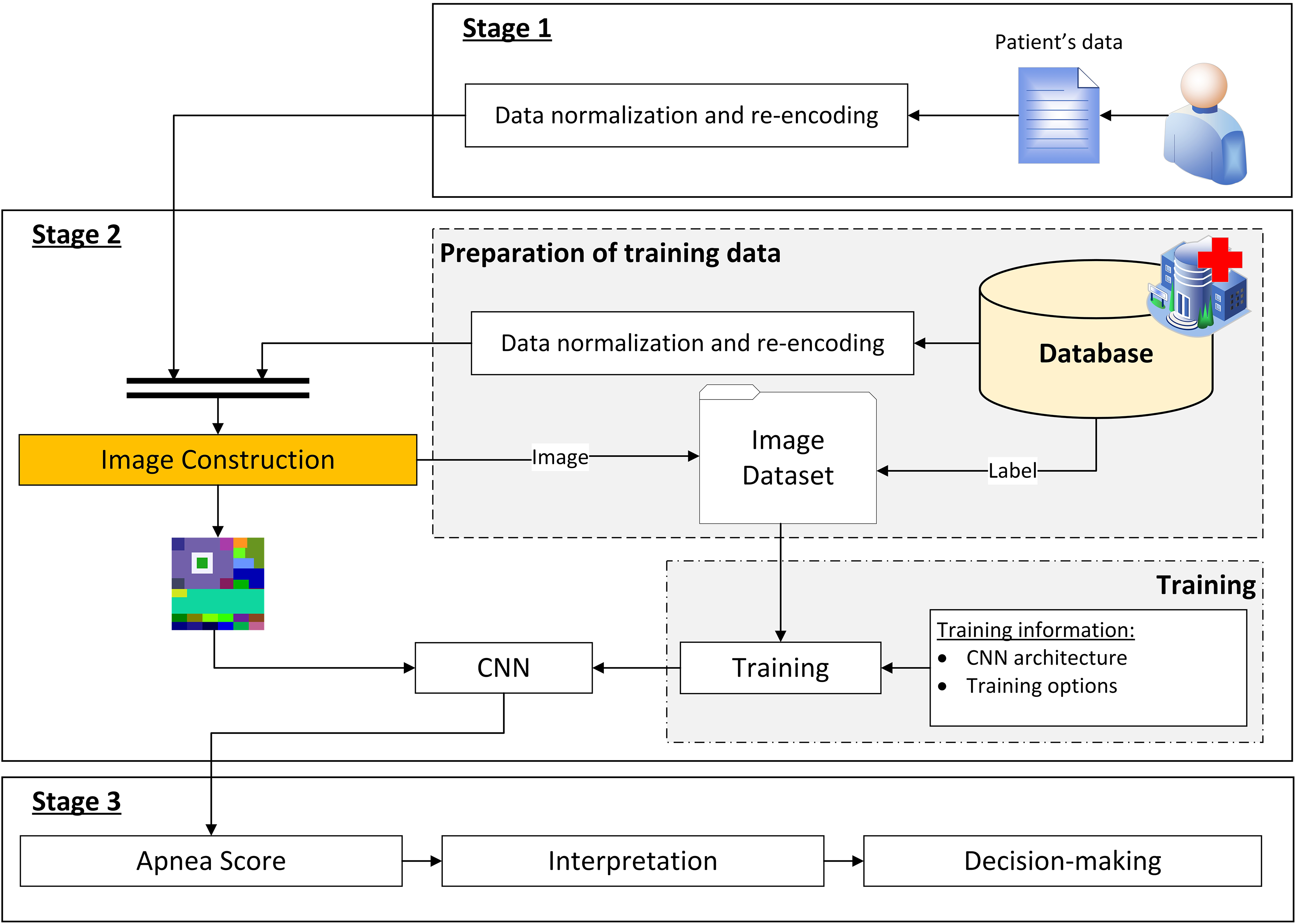
Flow diagram of the decision support system. It shows how the information advances through the different stages. Stage 1 deals with the collection of patient data. Stage 2 then deals with a new formalization of the data, representing it as an image, and then the inference process using a CNN. Finally, Stage 3 deals with the interpretation of the results obtained in Stage 2 and the generation of recommendations.

As shown in Figure 2, three main stages are identified, which are described below.

Stage 1: compilation of the patient's information

The first stage in this intelligent system refers to the process for compiling the patient's information, which has been already commented and introduced in Figure 1 of Database section.

Stage 2: data processing

Once the patient's information has been collected and structured, it is processed by the system. The first step involves the transformation of the initial information, which is in tabular format, into an image that condenses and agglutinates such patient's information. Subsequently, this image is used as input for a CNN, obtaining as output the Apnea Score, an indicator related to the hazard the patient has of being a moderate or severe OSA case.

The database used for CNN training was described in Database section. Before addressing such training, it is necessary to state that the database is also processed by transforming each patient’s data into a corresponding image. Starting from these images and the label associated with each of them, it is then possible to carry out the training of the CNN.

As already mentioned, this is a binary classification problem. The labels of the dataset were determined by setting a threshold value for the interpretation of AHI. Although a specific threshold value was set at 15, it is important to note that in the future, if deemed necessary by the medical team, as many other threshold levels could be established as necessary.

Stage 3: generation of alerts and decision-making

By representing the patients’ data encoded as images, it is possible to carry out their processing using a CNN, obtaining the Apnea Score value as its output.

In this last stage, the interpretation of the obtained Apnea Score value is addressed, determining the final label associated with the study patient. Based on this information, the medical team will be able to make the appropriate decisions regarding that patient.

Implementation of the system

Once the architecture of the intelligent decision support system has been introduced, this section deals with its implementation through a specific software artefact.

The implementation of the system has been carried out using the MATLAB^© software (version R2023a, Natick, MA, USA), supported by the App Designer module⁴⁶ for the development of the graphical interface, the Deep Learning Toolbox⁴⁷ for the design and implementation of deep neural networks, and an auxiliary script that allows implementing the elbow method⁴⁸ which is useful in this work to determine the optimal number of clusters using the k-means algorithm.

The equipment used for training the models consists of an Intel^© Core^© i9-10980HK CPU at 2.40 GHz, with an NVIDIA GeForce RTX 3070 Laptop GPU, and 32 GB of RAM.

A screenshot of the main screen of the developed tool is shown in Figure 3. As can be seen in it, there are three main areas: the Initial data collection panel where patient information is collected, the Data processing panel where the data is transformed into images and the Apnea Score is determined with the help of a CNN, and the Alert Generation & Decision Making panel where the Apnea Score is interpreted and the relevant alerts are generated.

Figure 3.

Screenshot of the main interface of the tool. The interface presents three main panels: Panel (1) is related to the collection of patient data; Panel (2) has two sub-panels, Panel (2.1) related to the transformation of the tabulated data into an image and Panel (2.2) related to the inference process; Panel (3) presents an interpretation of the results obtained and provides a recommendation regarding the patient's condition.

Information compilation

The patient-related data previously presented in Figure 1 are loaded into the application through the form shown in Figure 3, in the Initial data collection (1) panel.

It is important that the user verifies that no data have been omitted, or potential errors have happened that could reduce the precision of the system and increase the existing uncertainty level.

Data processing

Once the data have been entered into the form, they are processed by the intelligent system, as shown in Figure 3 in the Data Processing (2) panel.

First, the patient's data (initially structured in tabular format) is transformed into an image (this process is carried out in the Tabular Data to Image (2.1) panel of Figure 3). After that, the resulting image is processed by a CNN, obtaining as an output the Apnea Score (this process is carried out in the Convolutional Neural Network (2.2) panel of Figure 3).

Construction of the image

The image construction process consists of three phases which run sequentially, as shown in Figure 4.

Figure 4.

Process for the transformation of tabulated data into an image. The process consists of three main stages: In Stage 1, an empty image of 180 × 180 pixels is created, which will act as a container for the information; in Stage 2, four large sectors are created, which are coloured according to different clinical criteria (sex, detected apnoea, Epworth scale, age, body mass index, and neck circumference); in Stage 3, several sub-sectors are created on the previously created sectors, which will contain the information of the remaining variables (symptoms, drugs, previous pathologies, habits, and anthropometric data) and other additional information generated by clustering processes using k-means.

A detailed description of each of the phases is presented below. It is important to clarify that, in order to facilitate the image construction process, all numerical variables have been rescaled to the interval [0,1] by using a MIN–MAX type normalization. Likewise, the categorical variables have been re-encoded, transforming their different possible values into numbers. The binary variables are the simplest, assigning 1 or 0 to them depending on whether or not the patient presents each variable. In other cases in which the variables are categorical and not binary, as occurs with certain symptoms shown, Likert-like scales are used. These scales assign a score to each possible value, which is subsequently readjusted within the interval [0,1]. In this way, all the variables vary between 0 and 1 before the image is constructed, which is very convenient.

Phase 1: An empty 180 × 180 pixels image with three channels (R,G,B) is created. It is proposed to use square-shaped images since most CNN architectures rely on this image type, which will facilitate compatibility when using standard architectures (such as AlexNet,¹⁵ VGG,⁴⁹ ResNet,⁵⁰ etc.). Furthermore, this way the width and height of the image will be of equal importance, allowing the network to treat the different parts of the image in a uniform way. In any case, any other image size could be used as long as, after the appropriate rescaling, and avoiding deformations in the image proportions, it fits the CNN input layer size.

Phase 2: As shown in Figure 4, in this phase the image is divided into four sectors, each one of them associated to a characteristic or metric. These sectors are rectangular in shape, which favours their processing by CNNs. This is because the filters used in the convolution process are usually square or rectangular, which facilitates their application to orthogonal shapes, ensuring that the filters cover the different areas evenly, resulting in a more efficient process.

Sector 1: The indicated zone, depending on the patient's sex (man or woman), is painted with a pre-assigned colour value, randomly generated for each class.

Sector 2: The indicated zone is painted with a colour value which depends on the frequency that the patient presents apnoea incidents {No, Sometimes (twice or less per week), Often (more than twice per week) and Daily}. To calculate the colour value, two different values are established in the endings which are associated to the extreme values of the variable. In the case of the colours corresponding to the intermediate values, a chromatic gradient is implemented that extends between the extreme colour tonalities, assigning colour values in a proportional way, assuming that those values are equidistant in the chromatic space.

Sector 3: The indicated zone is painted depending on the value that the patient presents in the Epworth scale. To calculate the colour value, two different values are established in the endings, associated to the extreme values. The remaining values are calculated similarly to what was already commented in the previous point.

Sector 4: It is painted according to the patient's age, body mass index (BMI), and neck perimeter, as shown in Equation (1). The colour's R, G and B components are, respectively, functions of the patient's age, BMI and neck perimeter measurement.

f (n u m e r i c a l f e a t u r e) = (r e s c a l e d f e a t u r e) \cdot 255

(1)

Phase 3: Once the size of the image and the colours of the different sectors have been defined, that image is enriched with various patient characteristics as shown in Figure 4, and as detailed below. For this purpose, different sub-sectors are defined:

Sub-sector 1.1: This sub-sector is divided into two rows with six rectangles each, on which each of the symptoms reported by the patient are represented (for more information about them, refer to Database section, Figure 1). These symptoms, as already mentioned, are expressed using scales. Thus, each box is coloured with a colour depending on the value, using a chromatic gradient. As in previous cases, the extremes of the colour gradient are predefined.

Sub-sector 1.2: This sub-sector represents the drugs taken by the patient. To do this, it is divided into six rectangles, assigning a drug type to each one of them. The drug types are expressed as binary categorical data, and were previously discussed in Database section. If the patient takes the specific drug type, the corresponding rectangle is painted with a randomly pre-assigned colour.

Sub-sector 1.3: The process is similar to that already discussed for sub-sector 1.2. The sub-sector is divided into two rows with six rectangles each, on which each of the pathologies suffered by the patient is represented (for more information on these, refer to Database section, Figure 1). The patient's diseases are expressed as binary variables. Thus, if the patient suffers from that disease, the corresponding rectangle is painted with a pre-assigned colour, previously randomly generated.

Sub-sector 2.1: This sub-sector is related to patient's alcohol consumption. If the patient drinks alcohol, a rectangular bar with a size proportional in height to the associated alcohol consumption in grams of alcohol will be painted. In addition, the colour of the bar varies according to whether the consumption is occasional or daily, assigning a specific colour for each type of consumption.

Sub-sector 2.2: The smoking habit is represented in this sub-sector. If the patient smokes (or smoked in the past), a rectangular bar of a size proportional to the number of cigarette packs smoked per year will be painted. Likewise, the colour of the bar will be determined according to whether the patient is currently a smoker or has quit smoking, assigning a specific colour for each case.

Sub-sector 3.1: The size of this sub-sector is proportional to the patient's neck perimeter measure, and it is represented in the B-channel of the image, assigning the maximum value of 255 to the corresponding pixels.

Sub-sector 3.2: The size of this sub-sector is proportional to the patient's BMI, and it is represented in the G-channel of the image, assigning the maximum value of 255 to the corresponding pixels.

Sub-sector 3.3: The size of this sub-sector is proportional to the patient's age, and it is represented in the R-channel of the image, assigning the maximum value of 255 to the corresponding pixels.

Sub-sectors 4: For the calculation of these sub-sectors it is necessary to clarify that the clustering of several groups of data was previously carried out, using the k-means method,⁵¹ and determining the optimal number of clusters through the elbow method.⁵² In the case of sub-sector 4.1, general and anthropometric data (sex, age, BMI, and neck perimeter measure), in sub-sector 4.2 habits (alcohol and tobacco consumption), in sub-sector 4.3 diseases, in sub-sector 4.4 drugs taken, and in sub-sector 4.5 the symptoms evidenced, are respectively considered. After performing the clustering process, for each case, in each of the clusters the percentage of patients being moderate or severe OSA cases (i.e. having an AHI ≥ 15) is calculated. Then, in sub-sectors 4.1–4.5 the associated percentage is represented depending on the cluster to which the patient belongs in each case, represented in the image by means of a colour value, using for that a chromatic gradient. As in previous cases, the extremes of the colour gradient are pre-defined. On the other hand, for the determination of sub-sector 4.6 the clustering of the percentages reflected in sub-sectors 4.1–4.5 is addressed. K-means⁵¹ is also used for the clustering of the percentages, combined with the elbow method.⁵² In the latter case, a vector of random colours (represented by its RGB code), as many as clusters, is generated, assigning to sub-sector 4.6 the colour corresponding to each cluster in each case. Table 1 presents a summary of the data used in each sub-sector, together with the optimal number of clusters obtained after using the elbow method.⁵²

Table 1.

Data clustering. The data sets associated with each of the clusters generated in the third stage of the tabular data to image transformation process are presented, together with the optimal number of clusters obtained using the elbow method.

Sub-sector	Initial data	Optimal number of clusters
4.1	General and anthropometric data	9
4.2	Habits (alcohol and tobacco consumption)	9
4.3	Diseases	24
4.4	Drugs taken	6
4.5	Symptoms	104
4.6	Percentages of moderate or severe OSA case patients associated with sub-sectors 4.1, 4.2, 4.3, 4.4 and 4.5	53

Convolutional neural network: Apnea Score

Once the image has been obtained, its processing by the CNN is addressed. However, prior to that it is necessary to proceed to the training of the said CNN. To achieve this, we start with a set of 2225 images (90% of the initial database). The remaining images, corresponding to a 10% fraction of the dataset, are kept for testing purposes with the objective of evaluating the generalization capabilities of the model.

To exemplify the operation of the system, in this work it has been decided to use GoogleNet⁵³ as the CNN architecture of choice, adapting its output for two classes. To speed up and simplify the training of the network, we start with a pre-trained network on the ImageNet dataset,⁵⁴ so that its weights are not randomly initialized. In any case, if deemed appropriate in the future, any other CNN architecture could be used if the results obtained are considered as satisfactory.

The network was trained using MATLAB Deep Learning Toolbox. The training configuration of the model is shown next in Table 2. A cross-validation strategy⁶ was used for training with a k equal to 10 folds. In each of the 10 iterations, the model was trained using nine folds as the training set and its performance was evaluated on the remaining fold, which acted as the validation set. Figure 5 shows the ROC curves and AUC values for each of the folds, allowing the stability of the model to be validated, with minimal differences between them. During the iterations of the k-fold cross-validation, the model that performed best in its validation fold was selected. This model is considered to be representative of the maximum performance obtained during the cross-validation process.

Figure 5.

ROC Curves for each fold in cross-validation (k = 10).

Table 2.

Training configuration of the network.

Hyperparameter	Value	Comment
Optimizer	Adam	–
Mini-batch size	128	–
Max epochs	40	–
Learning rate	0.0001	–
Validation frequency	Each iteration	–
Validation patience	50	Determines the maximum number of occurrences where the loss on the validation set can either match or exceed the previously recorded minimum loss, subsequently leading to the termination of the neural network training process.
Output network	Best validation loss	Selects those parameters of the neural network corresponding to the training iteration with the lowest validation loss.

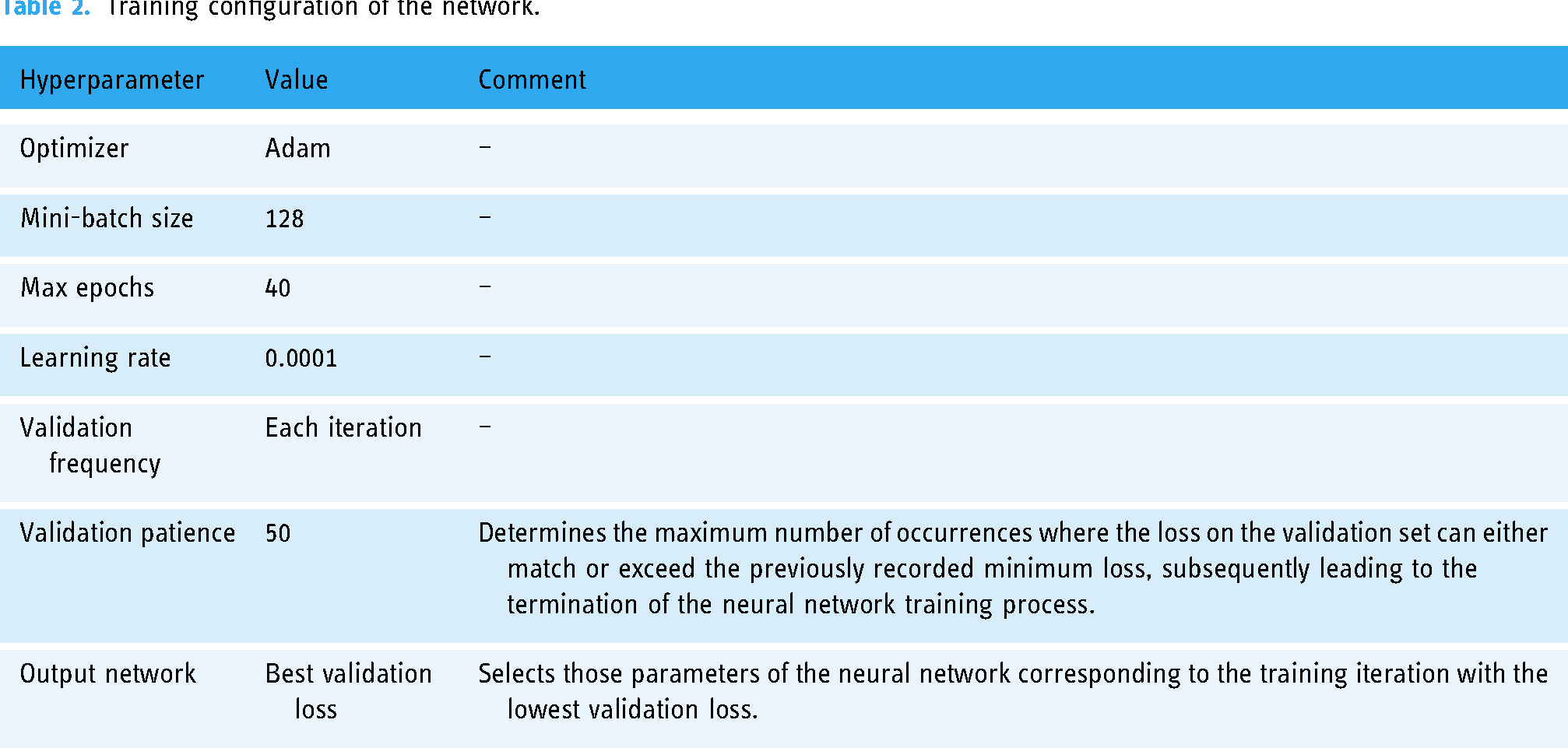
Once the network has been trained, the Apnea Score is obtained at its output in the presence of new images. As already mentioned, this indicator represents the risk of a patient being a moderate or severe OSA case. It is a value within the interval [0,1], although for practical reasons it will later be re-scaled between 0 and 100.

In order to facilitate the interpretation of the results obtained at the CNN output, it is necessary to establish a threshold level that allows discrimination between the two classes (“Non-OSA or mild OSA case” and “Moderate or severe OSA case”).

To achieve this, a graphical optimization process will be undertaken, aimed to highlight the threshold value that maximizes the associated Matthews correlation coefficient (Mcc) value^55–57 on the test dataset. Equation 2 shows the expression of the Mcc. The acronyms in the equation are as follows: TN = true negatives, FN = false negatives, TP = true positives and FP = false positives.

M c c = \frac{T N \cdot T P - F N \cdot F P}{\sqrt{(T P + F P) \cdot (T P + F N) \cdot (T N + F P) \cdot (T N + F N)}}

(2)The use of Mcc has been chosen instead of other metrics, such as precision, since the data set used is unbalanced. This coefficient is a particularization of the Phi coefficient,^55–57 and only shows successful values when satisfactory results are obtained for the four characteristic values in the confusion matrix.

Figure 6 represents the different Mcc values associated with the different threshold values. It is observed that Mcc is maximized for a threshold value of 0.68, with an associated Mcc value of 0.48.

Figure 6.

Determination of the optimal cut-off point for the CNN. This is a graphical optimization process where the Matthews correlation coefficient is calculated for each threshold on the score obtained at the CNN output on the test set.

Figure 7 shows the ROC curve of the CNN on the testing dataset, highlighting the point of optimal performance, associated with the threshold value of 0.68 previously calculated. At this point, values are shown for the sensitivity of 0.76, and for the specificity of 0.73.

Figure 7.

ROC curve on the testing dataset and operation point. The operating point was obtained through a graphical optimization process based on the Matthews correlation coefficient.

In addition to the determination of the Apnea Score in Panel 2.2 of Figure 3, a new visualization is also presented that combines the image agglutinating the patient's data with a superimposed colour map based on the gradient-weighted class activation mapping (Grad-CAM) method.⁵⁸ Its use is intended to highlight those regions having the greatest influence on the predictions, with the goal of improving the image. In any case, it is important to clarify that its use is not intended to identify which independent variables have a greater influence on the prediction.

Comparison with other conventional machine learning models

Although this article focuses on explaining the design and development of a new model of an intelligent system, it may be useful, especially in assessing its potential and benefits, to make a comparison of the model presented with others already existing in the state of the art. This is only an illustrative analysis, since it is clear that an exhaustive comparison should be made, tested, validated, and contrasted with models at similar stages of maturity. However, as noted above, an estimate of the results on a given set will serve as a representative example of its usefulness. Therefore, this section presents a complementary analysis of some of the most widely used machine learning models in the field of defining intelligent decision support systems. For this purpose, and given the enormous diversity of models, we have chosen to select the most representative of three broad groups of models, which are not exclusive but complementary, following the recommendations of Peter Flach.⁵⁹ These groups include models that can be categorized as geometric, probabilistic, or logical. To make the comparison practical and effective, several tests were carried out using the MATLAB Classification Learner app,⁶⁰ which groups together models from the groups described above. The data set is the one already discussed in Database section, reserving 10% of the data for testing and training the models with the remaining 90% using a cross-validation strategy with k equal to 10 as described above.

To ensure homogeneity in the comparison, the data pre-processing was similar to that used before image construction: all numerical variables were rescaled to the interval [0,1] using a MIN–MAX type normalization. Similarly, categorical variables were recoded by transforming their different possible values into numbers. Binary variables were treated in a simple way, assigning 1 or 0 depending on whether the patient had the characteristic or not. In other cases, where the variables were categorical but not binary, as in the case of certain symptoms, Likert scales were used.

Table 3 gives a summary of the different algorithms used in the training process, using the default settings in the MATLAB Classification Learner app, and the results obtained on the test set, expressed in terms of AUC. As can be seen, k-neighbour models, support vector machines (SVM), naïve Bayes, decision trees, and even basic artificial neural network models have been used.

Table 3.

Comparison with other conventional machine learning models.

Model	Comment	AUC in test
Coarse decision tree	Maximum number of splits = 4; split criteria = Gini's diversity index	0.68
Medium decision tree	Maximum number of splits = 20; split criteria = Gini's diversity index	0.72
Fine decision tree	Maximum number of splits = 100; split criteria = Gini's diversity index	0.67
Bagged trees	Decision tree-based assembly; maximum number of splits = 2224; number of learners = 30	0.76
Naïve Bayes	—	0.70
SVM	C parameter (box constraint level) = 1; kernel scale mode = automatic; kernel = Linear	0.75
SVM	C parameter (box constraint level) = 1; kernel scale mode = automatic; kernel = quadratic	0.72
SVM	C parameter (box constraint level) = 1; kernel scale mode = automatic; kernel = cubic	0.67
Coarse KNN	Number of neighbours = 100; distance = Euclidean	0.74
Medium KNN	Number of neighbours = 10; distance = Euclidean	0.67
Narrow neural	Number of fully connected layers = 1; number of neurons = 10; activation function = ReLU; iteration limit = 1000	0.68

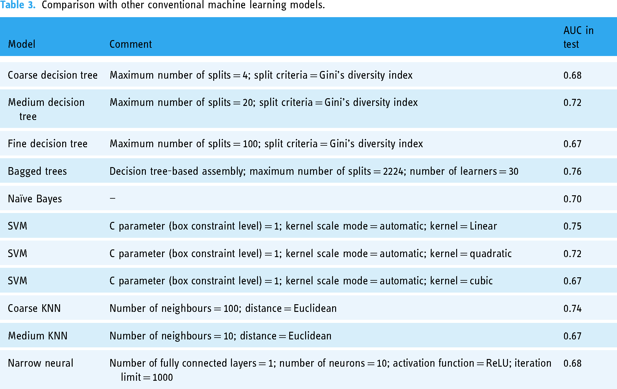
From the analysis of the results shown in Table 3, it can be seen that none of the models studied reaches ROC curves above 0.8, with only the bagged trees model exceeding the 0.75 AUC threshold. All the models that exceed 0.7 AUC can be considered as moderately successful in classification, although they are worse than the proposed model. Models above 0.75, such as bagged trees, obtain better results, reflecting, for example, the usefulness of the use of ensemble strategies. However, all the values are still lower than those of our proposal, which achieves an AUC close to 0.8, showing a higher prediction accuracy, although its validation and development are still in the initial stages.

Generation of alerts and decision making

Once the Apnea Score is determined, its value is interpreted based on the threshold value calculated in the previous section, thus obtaining the label associated with the patient (“Non-OSA or mild OSA case” and “Moderate or severe OSA case”).

This information is displayed in the Alert generation and Decision Making panel (3) shown in Figure 3.

Case study

To facilitate the understanding of the operation of the intelligent system, and to highlight its potential in clinical decision making, this section presents a practical case study. It should be noted that the case study is only a proof of concept and is in no way a comprehensive validation of the applicability and usability of the method.

A detailed description of the architecture of the intelligent system (see Figure 2 for more information) and its implementation has been presented in Materials and methods section of this paper. Regarding its implementation, Figure 4 and Table 1 are fundamental to understand the process of image generation from tabular data, which is the main novelty and strength of the present work. It is also important to point that a reasoning system based on a DL model, namely a CNN, is used. This model is based on GoogleNet, although any other CNN with adequate behaviour could be valid. A summary of the hyperparameters used during the training of this model is presented in Table 2. On the other hand, once the model has been contextualized, its performance measures need to be addressed. In this regard, Figures 6 and 7 are crucial: the first determines the threshold for interpreting the score obtained at the CNN output, which allows to distinguish between patients with moderate-to-severe cases and those with mild or no cases, while the second shows the ROC curve of the CNN over the test set, highlighting the operating point. It is important to note that a dataset from the Pulmonary Department of the Hospital Álvaro de Vigo was used, and if a different database was used, the thresholds would have to be revised and updated accordingly.

Compilation of the patient's data

Table 4 shows the data of the patient to be studied. It is important to clarify that this data was not used in the training of the system, and that the patient presented an AHI value of 6.4 at the sleep tests. This indicator will be considered later to analyse the insights generated by the intelligent system.

Table 4.

Data of the study patient.

Group 1	General and anthropometric data
	Sex	Woman
	Age	30 years old
	BMI	55.27
	NCL	38 cm
	Habits of the patient
	Smoker	No
	Packs-per-year index	–
	Drinking habits	No
	Grams of alcohol	–
	Diseases
	Hypertension	No
	Resistant hypertension	No
	ACVA	No
	ACVA less than a year ago	No
	Diabetes	No
	Ischaemic heart disease	No
	COPD	No
	Need for home oxygen-therapy	No
	Rhinitis	No
	Depression	Yes
	Atrial fibrillation	No
	Heart failure	No
	Drug treatments
	Benzodiazepines	Yes
	Antidepressants	Yes
	Neuroleptics	No
	Antihistamines	No
	Morphic	No
	Relaxing/hypnotic drugs	Yes
Group 2	Interview
	Intra-sleep awakening	Frequently (>2 times/week)
	Snore awakening	No
	Asphyxia awakening	No
	Short-of-breath awakening	No
	Unrefreshing sleep	Daily
	Daily tiredness	Daily
	Lack of focus	Often (>2 times/week)
	Perceived drowsiness	Often (>2 times/week)
	Morning dullness	Often (>2 times/week)
	Nocturia	Sometimes (≤2 times/week)
	Snorer	No
	High-intensity snorer	No
	Evidenced apnoeas	No
	Epworth scale	16

Note. The data are summarised in two groups, firstly in Group 1, those related to the digital health record, and secondly in Group 2, those related to the patient’s symptomatology.

Once the data have been collected, they are entered into the application to be processed by the intelligent system, as shown in Panel 1 of Figure 8.

Figure 8.

Screenshot of the software application in the case study.

Data processing

Once the data have been entered into the application, their processing is addressed. In Panel 2.1 of Figure 8 the data transformation process is carried out, representing them as an image. A detailed description of the image generation process is given in Data processing section. Subsequently, in Panel 2.2 the image is processed by the CNN, thus obtaining the Apnea Score which shows a value of 50.97 for this case.

Also, an image is shown with a superimposed colour map highlighting certain areas that have been key to the proposed prediction. In this case, those areas result to be Cluster 1: general and anthropometric data, habits, and symptoms. For more information on the image and its different zones, it is recommended to revisit Figure 4. It is important to remember that the purpose of using Grad-CAM in our case is not to identify which independent variables have the greatest influence on prediction, but to identify which areas of the image are most important for prediction.

Generation of alerts and decision making

Finally, the interpretation of the Apnea Score is addressed, which presents a value lower than the previously calculated threshold, so the system indicates that the patient, either is not, or is a mild OSA case, as can be seen in Panel 3 of Figure 8.

Taking into account the system recommendation, it seems that the patient does not suffer from the disease, or suffers mild case of it. This is a plausible prediction, and one that fits with the real results, given that the patient resulted in an AHI value of 6.4 in the sleep test.

Discussion

When working with inductive reasoning models such as those at the very basis of DL techniques, we must deal with the categorization of the dimensionality of the starting datasets. In particular, DL tools are especially designed for the management, processing and inference on these (sometimes huge) volumes of data, resulting in the identification of very specific generalization models that tend to overfitting, or even to over-optimistic predictive estimations. This work focuses its main contributions on a new proposal for data formalization based on the elaboration of images with graphical matrix samples of data volumes of high dimensionality, in the sense of the number of independent variables or characteristics. In this way, statistically significant relationships between variables can be represented and qualified using visual elements such as colour gradients or contrasts, which are more easily analysed and traced by advanced DL models than by conventional learning models.

It is a work, therefore, of data formalization so that we develop the capability to represent the information present in the original data in a more compact and traceable way without giving up the ontological meaning of the new structure, or quasi-symbol, that represents such information. Thus, in this article these new structures will be images obtained from the initial data. The logical and, as was said, ontological nature of the image as a representation of information is evident, claiming that it may contain a figurative representation of the information present in the original data. Figurative must be understood regarding its form and colour, with all the available nuances (brightness, contrast, tone, etc.), while keeping its association with each part of the same information present, implicitly or explicitly, in the initial data.

But the very fact of formalization would not be enough to improve the capability for fine-tuned generalization and capture of the complexity of DL models without resourcing to network topologies, such as CNNs with high and reputed capabilities for processing data structures in image form. These networks take advantage of a discrete image layout to apply convolution operations that transform and adapt that image according to certain filters, in such a way that they are able to realize complex patterns between these images and their corresponding labels in supervised learning strategies. It is precisely this combination that stands out in this work. Formalizing a dataset, creating an image that without excessive loss or conditional uncertainty represents the initial information, and using the set of images in convolutional network training not only represents a unique evolution in inductive intelligent systems, but also extends and facilitates their use by avoiding the inherent problems associated with the excessive dimensionality of the datasets.

In general, when working with tabular data in traditional learning models, as the volume of data increases, it becomes difficult to find clear and logical boundaries in the instance space, which can accentuate bias and variance. In this sense, by transforming data into images, better dimensionality management is achieved, reducing the bias and variance^6–9 associated with traditional models. If we add to this the use of DL models, generally based on convex optimization problems,⁸ which work with large chains of summands in regression and classification processes, we can overcome many of the difficulties associated with the same process using traditional statistical models.

Having said this, we can specify the innovative features that will be included in our proposal:

Image shape: The shape is one of the elective characteristics of the data structure created. Its choice is not random, but is due to the nature and own operation of the filters in the convolution operations, usually referred to Cartesian operations understood as matrix multiplications on larger square or rectangular matrices. Hence, the prioritized and logical choice is to use square or rectangular images. Furthermore, square shapes in input images are generally more relevant in this case, due to the usual architecture pre-training processes. This facilitates compatibility with such standard architectures (such as AlexNet,¹⁵ VGG,⁴⁹ ResNet,⁵⁰ etc.), which significantly reduces training times and the required computational capacity.

Data layout: Once choice for the image's external shape has been justified, the choice of the internal arrangement should be reasoned. In this work it is proposed that each variable be represented in the image through the use of a rectangle of variable area positioned in a certain region of such image, with the objective of emulating a grid structure. In this way, it tries to contribute to reducing the computational complexity, since if the image contains orthogonally separable regions, it will be easier to process them and to favour the feature extraction by optimizing the convolution filters. In addition, the choice of GoogleNet is also very convenient, as it addresses an implicit optimization of computational resources by incorporating 1 × 1 convolution filters,^53,61 which allows to reduce the dimension before applying larger filters and the structures of the inception modules. Therefore, the inclusion of orthogonally separable zones in the images can theoretically improve the efficiency and accuracy of GoogleNet, although its design also focuses on optimizing the generalization. In addition, different colours (which have been randomly selected) have been used in each of the rectangles to represent the different casuistry, increasing the formalization capabilities of the structure. As before, the reason for this is not accidental. The convolution filter or kernel slides through the image sequentially depending on values such as the stride and the size of the filter itself. Analysing these values, it is considered that a regular arrangement of rectangular-shaped information structures categorized by their colour would always remain under the influence of the kernel's sliding process, adjusted in any case by the set stride value and, as said, the size of the filter. This guarantees the representativeness of the collected information, i.e., edges and colours would be gathered under the influence of the size and characteristics of colour kernels ensuring their influence on the generalization process. Certainly, the distribution of these rectangular structures could even be parameterized under the condition of a further optimizable hyper-parameter in the training and validation process of the network.

Implicit data formalization: The process of transforming the tabulated data into the image is carried out in four phases. After creating an empty image in the first phase, in the second phase four rectangular sectors are defined on the image. Each of them represents information of great relevance in the diagnostic process according to established medical criteria. Thus, Sector 1 represents the patient's sex (several studies suggest that man sex is an important OSA-related risk factor). Sector 2 represents the evidenced apnoeas; in this sense, sleep tests aim to quantify the number of apnoea–hypopnoea events that the patient presents during sleep, and this is why, a priori, this variable is considered of great importance since it could help to identify those patients who present this type of events more frequently. Sector 3 represents the Epworth scale, an indicator that aims to evaluate daytime sleepiness in adults; this is a highly relevant metric, as it can reveal individuals with poor quality, non-refreshing sleep. Finally, Sector 4 represents a composition of age, body mass index and neck perimeter; these are anthropometric data of great relevance in the diagnosis of OSA. Once this has been done, in Phase 3 the rest of the variables are represented by using smaller rectangles over the different sectors, grouped according to their typology in different sub-sectors (e.g. symptoms, drugs taken, previous diseases, habits, etc.). Lastly, in Phase 4 the image gets enriched with information obtained through a previous clustering process supported by the use of the k-means method. The use of unsupervised learning models, in this case through clustering approaches, allows the identification of latent patterns in the data, grouping similar observations. By incorporating not only these groupings, but also the relationships between them, a more complete and detailed representation of the starting data is achieved, adding an additional layer of complexity to the model. By doing so, it is possible to find relationships that may not be evident in the starting data set, that are difficult to capture with traditional learning models, and that can be easily integrated into an image, thus facilitating the construction of a more robust model that is less prone to be affected by noise and overfitting.

Furthermore, it is important to clarify that the network topology to be used is not a fundamental issue, at least in this paper. We have chosen to use GoogleNet, although any other topology could be used. This is because this proposal focuses on the utility of converting tabular data into images, rather than on the selection of a particular network to process these images. It would be possible to use simpler topologies than GoogleNet, or more computationally complex ones, which would influence the network's ability to detect greater complexity in image construction, which the authors believe strengthens this proposal, since it would be possible to translate large amounts of data into more complex images that can be analysed by a CNN.

It is also worth highlighting the results obtained from a comparison of the intelligent system with other learning models, representative of the groups of algorithms categorized as geometric, probabilistic, or logical. Although the methodology presented is at a first proof-of-concept stage, the comparison shown in Table 3 suggests that the predictive capacity of our proposal is at least equal to or better than that of other widely used models. This allows us to assess its potential for growth and improvement, and to establish a measure of its technical relevance.

Finally, once the images have been created, a tool such as Grad-CAM is used to improve the data layout and avoid the optimization of the parameterization described above. Its use makes it easier to visualize the areas that the network considers important for making predictions, without attempting to determine the influence of the independent variables of the problem or to explain in detail why. When using a CNN as an inference engine in an intelligent system, one must assume an inherent difficulty in interpreting its predictions, a difficulty related to the complexity of the model itself.^62,63 Although there are other explanatory artificial intelligence tools that could be useful, such as SHAP (SHapley Additive exPlanations),⁶⁴ which offer a more detailed approach to the influence of data on predictions, in general they all take an inductive approach to knowledge that is ephemeral and context-dependent, which does not fit the purpose of this work. In this framework, Grad-CAM is used to illustrate these relationships in a visual way, providing insight into specific activations, without pretending to offer an exhaustive justification from a medical point of view, which could be useful:

Validating the representation of the features: Through the visual inspection process, it is possible to determine if the features incorporated into the images are being correctly captured and used by the model in the predictions.

Identifying problem areas in the image and model errors: Visual inspection, together with the model predictions, facilitates the identification and correction of possible inconsistencies between the tabulated features and the generated visual representations, which contributes to continuous model improvement.

Conclusions

In this paper we have described the design, development, and proof of concept of an intelligent system to predict possible sleep apnoea cases. In contrast to other works in the same line, a novel model of formalization and representation of information based on the accommodation of high-dimensional data into new structures in the form of two-dimensional images has been proposed. This approach has not only lowered the harmful effects associated with datasets with a large number of initially independent variables, but has also improved the adaptation of DL models to the inductive capture of the nonlinear relationships of these variables with the proposed categories. The results derived from the proof of concept show high classification accuracy with ROC curve areas close to 0.8, determining classifiers of substantial diagnostic reliability. This value was compared with those obtained by applying various state-of-the-art models, none of which achieved a similar result to our proposal. This opens up a set of unique and potentially achievable opportunities to represent massive datasets in perfectly identifiable structures that could be processed by deep network topologies, which as observed in the results will improve the generalization capabilities of these on the initial data.

However, we must consider several limitations that could impact the interpretation and application of our findings:

Reduced dimensionality and overfitting: Working in more limited dimensionality spaces reduces training times and datasets but introduces a tendency towards inevitable overfitting. This overfitting can increase as the complexity of the generated image rises, depending on the size of the initial dataset. In an overly optimistic framework, this might unnecessarily augment the complexity of the model and lead to poor results in test runs. To mitigate these effects, strategies such as applying regularization techniques or incorporating validation during the model training phase, using dropout layers during training, or even optimizing stride and padding values during training could be employed.

Challenges in data formalization and image creation: The process of image creation itself is not devoid of challenges. The definition of shape, internal composition, and colour of the images follows a parallel rationale to the use of kernels in convolution layers. However, a detailed analysis of these elements, their sequencing in the network architecture, and their internal stride settings might suggest the need for different shapes, compositions, or even colours. The choice of the correct geometric arrangements and colour schemes can significantly affect the efficiency with which the different convolution filters identify and interpret the initial features, potentially affecting the accuracy of the algorithm. For example, inappropriate colour coding could obscure important distinctions between classes, leading to misclassifications. The objective parameterization of the layout and the establishment of effective shape factors are crucial. These adjustments will allow for the incorporation of new hyperparameters aimed at improving network performance.

Choice of convolutional network model: This proposal focuses on the utility of converting tabular data into images, rather than on the selection of a particular network to process these images. The choice of architecture is important because different network topologies have different capabilities for capturing and modelling features from complex images. It would be possible to use topologies that are simpler than GoogleNet, or more computationally complex, which would affect the ability of the network to recognize greater complexity in image construction.

Interpretation of model predictions: The ability to interpret the predictions of highly complex models such as DL is virtually non-existent.^62,63 Knowing the reason for the predictions and their implications is a very relevant issue in medical settings, such as the diagnosis of obstructive sleep apnoea. In this proposal, Grad-CAM has been used to facilitate the visualization of the most relevant areas of the images in the inference process with a CNN. However, although Grad-CAM provides a useful visualization of the features highlighted by the CNN in its prediction, it does not provide a direct interpretation, nor does it attempt to explain why. The technique shows active areas related to network output but does not explain why these areas are medically relevant, which was not the purpose of this work, although it could certainly limit the usefulness of our methodology in contexts where interpretability is mandatory. To achieve this, one could opt for the use of other explainable artificial intelligence (XAI) approaches,⁶⁵ although these generally take an inductive and ephemeral approach to knowledge. That is, they would allow statistical reasoning between predictor and predicted variables, but they would not be able to create permanent, unchanging, and structural knowledge.

Each of these limitations points towards specific areas for future research, where methodological and architectural adjustments can potentially enhance the robustness and applicability of our model in clinical and research contexts.

Footnotes

Contributorship

The authors confirm contribution to the paper as follows: study conception and design: MCG and ACC; data collection: MTD, MMA, and AFV; analysis and interpretation of results: MCG, MTD, MMA, ACC, JCP, and AFV; draft manuscript preparation: MCG. All authors reviewed the results and approved the final version of the manuscript.

Declaration of conflicting interests

The authors declared no potential conflicts of interest with respect to the research, authorship, and/or publication of this article.

Ethical approval

The ethics committee of Galicia approved this study (2022/256, 2 July 2022).

Funding

This research was supported by the Galicia Sur Health Research Institute under the “II Convocatoria Intramural de Axudas á Investigación Biomédica 2023” with the project code CI23-05.

Guarantor

MCG.

ORCID iD

Manuel Casal-Guisande

References

Miotto

Wang

, et al. Deep learning for healthcare: review, opportunities and challenges. Brief Bioinform 2018; 19: 1236–1246.

Saeys

Inza

Larrañaga

. A review of feature selection techniques in bioinformatics. Bioinformatics 2007; 23: 2507–2517.

Cheng

Wang

, et al. Feature selection: a data perspective. ACM Comput Surv 50. Epub ahead of print 1 December 2017. DOI: https://doi.org/10.1145/3136625.

Casal-Guisande

Comesaña-Campos

Núñez-Fernández

, et al. Proposal and definition of an intelligent clinical decision support system applied to the prediction of dyspnea after 12 months of an acute episode of COVID-19. Biomedicines 2024; 12: 854.

Casal-Guisande

Comesaña-Campos

Dutra

, et al. Design and development of an intelligent clinical decision support system applied to the evaluation of breast cancer risk. J Pers Med 2022; 12: 169.

Bonaccorso

. Machine learning algorithms: popular algorithms for data science and machine learning. 2nd ed. Birmingham, UK: Packt Publishing Ltd., 2018.

Zhou

Z-H

. Machine learning. Singapore: Springer Singapore, 2021. Epub ahead of print 2021. DOI: https://doi.org/10.1007/978-981-15-1967-3.

Bach

. Breaking the curse of dimensionality with convex neural networks. J Mach Learn Res 2017; 18: 1–53.

Berisha

Krantsevich

Hahn

, et al. Digital medicine and the curse of dimensionality. npj Digital Med 2021; 4: 1–8.

10.

Lecun

Bengio

Hinton

. Deep learning. Nature 2015; 521: 436–444.

11.

Goodfellow

Bengio

Courville

. Deep learning. Cambridge, MA, USA: MIT Press, 2016.

12.

Schmidhuber

. Deep learning in neural networks: an overview. Neural Netw 2015; 61: 85–117.

13.

Bengio

. Deep learning of representations: looking forward. In: Lecture notes in computer science (including subseries lecture notes in artificial intelligence and lecture notes in bioinformatics), 2013, pp.1–37. 7978 LNAI. Berlin, Heidelberg, Germany: Springer.

14.

Fernando

. Redes neuronales & deep learning. [Independently published], 2018.

15.

Krizhevsky

Sutskever

Hinton

. ImageNet classification with deep convolutional neural networks. Adv Neural Inf Process Syst 2012; 25: 1097–1105.

16.

Simonyan

Zisserman

. Very deep convolutional networks for large-scale image recognition. In: 3rd international conference on learning representations, ICLR 2015 – conference track proceedings, https://arxiv.org/abs/1409.1556v6 (2014, accessed 11 October 2023).

17.

Liu

Yang

, et al. A survey of convolutional neural networks: analysis, applications, and prospects. IEEE Trans Neural Netw Learn Syst 2022; 33: 6999–7019.

18.

O’Shea

Nash

. An introduction to convolutional neural networks. Int J Res Appl Sci Eng Technol 2015; 10: 943–947.

19.

Wang

Kuen

, et al. Recent advances in convolutional neural networks. Pattern Recognit 2018; 77: 354–377.

20.

Salehinejad

Sankar

Barfett

, et al. Recent Advances in Recurrent Neural Networks. https://arxiv.org/abs/1801.01078v3 (2017, accessed 19 October 2023).

21.

Zhu

Brettin

Xia

, et al. Converting tabular data into images for deep learning with convolutional neural networks. Sci Rep 2021; 11: 1–11.

22.

Damri

Last

Cohen

. Towards efficient image-based representation of tabular data. Neural Comput Appl 2023; 36: 1023–1043.

23.

Prisant

Dillard

Blanchard

. Obstructive sleep Apnea syndrome. J Clin Hypertension 2006; 8: 746–750.

24.

Goyal

Johnson

. Obstructive sleep Apnea diagnosis and management. Mo Med 2017; 114: 120.

25.

Punjabi

. The epidemiology of adult obstructive sleep apnea. Proc Am Thorac Soc 2008; 5: 136–143.

26.

Kapur

Auckley

Chowdhuri

, et al. Clinical practice guideline for diagnostic testing for adult obstructive sleep apnea: an American Academy of Sleep Medicine Clinical Practice Guideline. J Clin Sleep Med 2017; 13: 479–504.

27.

Zheng

Eniola

Wang

. Machine learning for colorectal cancer risk prediction. In: 2021 international conference on cyber-physical social intelligence, ICCSI 2021. Epub ahead of print 2021. DOI: https://doi.org/10.1109/ICCSI53130.2021.9736248.

28.

Zheng

Wang

. Predicting ICU length of stay for patients with diabetes using machine learning techniques. In: Proceedings of the international conference on cyber-physical social intelligence, ICCSI 2022 , 2022, pp.417–422. Nanjing, China: IEEE.

29.

Cerqueiro-Pequeño

Casal-Guisande

Comesaña-Campos

, et al. Conceptual design of a new methodology based on intelligent systems applied to the determination of the user experience in ambulances. In: ACM international conference proceeding series , 2021, pp.290–296. New York, NY, USA: Association for Computing Machinery.

30.

Casal-Guisande

Comesaña-Campos

Cerqueiro-Pequeño

, et al. Design and definition of a new decision support system aimed to the hierarchization of patients candidate to be admitted to intensive care units. Healthcare 2022; 10: 587.

31.

Casal-Guisande

Cerqueiro-Pequeño

Comesaña-Campos

, et al. Conceptual proposal of a hierarchization system for patients candidate to intensive care units in health catastrophe situations. In: Eighth international conference on technological ecosystems for enhancing multiculturality, 2020, pp.496–500. New York, NY, USA: Association for Computing Machinery.

32.

Casal-Guisande

Cerqueiro-Pequeño

Comesaña-Campos

, et al. Proposal of a methodology based on expert systems for the treatment of diabetic foot condition. In: Eighth international conference on technological ecosystems for enhancing multiculturality , 2020, pp.491–495. New York, NY, USA: Association for Computing Machinery.

33.

Casal-Guisande

Bouza-Rodríguez

Comesaña-Campos

, et al. Proposal and definition of a methodology for remote detection and prevention of hypoxemic clinical cases in patients susceptible to respiratory diseases. In: Proceedings of the seventh international conference on technological ecosystems for enhancing multiculturality , 2019, pp.331–338. New York, NY, USA: Association for Computing Machinery.

34.

Cerqueiro-Pequeño

Comesaña-Campos

Casal-Guisande

, et al. A proposal for using active contour parametrical models in Cobb angle determination. In: Ninth international conference on technological ecosystems for enhancing multiculturality (TEEM’21) , 2021, pp.297–304. New York, NY, USA: Association for Computing Machinery.

35.

Côrte-Real

Dutra

Rocha

. On applying probabilistic logic programming to breast cancer data. In: Lachiche

Vrain

(eds) Inductive logic programming. Cham: Springer International Publishing, 2018, pp.31–45.

36.

Ferreira

Dutra

Salvini

, et al. Interpretable models to predict breast cancer. In: 2016 IEEE international conference on bioinformatics and biomedicine, BIBM 2016 , 2017, pp.1507–1511. Piscataway, NJ, USA: Institute of Electrical and Electronics Engineers Inc.

37.

Casal-Guisande

Álvarez-Pazó

Cerqueiro-Pequeño

, et al. Proposal and definition of an intelligent clinical decision support system applied to the screening and early diagnosis of breast cancer. Cancers (Basel) 2023; 15: 1711.

38.

Mencar

Gallo

Mantero

, et al. Application of machine learning to predict obstructive sleep apnea syndrome severity. Health Informatics J 2020; 26: 298–317.

39.

Sun

Chiu

Chuang

, et al. A prediction model based on an artificial intelligence system for moderate to severe obstructive sleep apnea. Sleep Breathing 2010; 15: 317–323.

40.

Ramesh

Keeran

Sagahyroon

, et al. Towards validating the effectiveness of obstructive sleep apnea classification from electronic health records using machine learning. Healthcare 2021; 9: 1450.

41.

Zoroglu

Turkeli

. Fuzzy expert system for severity prediction of obstructive sleep apnea hypopnea syndrome. J Cogn Systems 2017; 2: 37–43.

42.

Matthews

Kwiatkowska

Matthews

. A preliminary fuzzy model for screening obstructive sleep apnea. In: Proceedings of the 2013 Joint IFSA World Congress and NAFIPS Annual Meeting, IFSA/NAFIPS 2013 2013, pp.187–191. Piscataway, NJ, USA: Institute of Electrical and Electronics Engineers.

43.

Casal-Guisande

Torres-Durán

Mosteiro-Añón

, et al. Design and conceptual proposal of an intelligent clinical decision support system for the diagnosis of suspicious obstructive sleep apnea patients from health profile. Int J Environ Res Public Health 2023; 20: 3627.

44.

Casal-Guisande

Ceide-Sandoval

Mosteiro-Añón

, et al. Design of an intelligent decision support system applied to the diagnosis of obstructive sleep apnea. Diagnostics 2023; 13: 1854.

45.

Casal-Guisande

Cerqueiro-Pequeño

Bouza-Rodríguez

J-B

, et al. Integration of the Wang & Mendel algorithm into the application of fuzzy expert systems to intelligent clinical decision support systems. Mathematics 2023; 11: 2469.

46.

MATLAB App Designer – MATLAB & Simulink. https://es.mathworks.com/products/matlab/app-designer.html (accessed 10 June 2024).

47.

Deep Learning Toolbox – MATLAB. https://es.mathworks.com/products/deep-learning.html (accessed 10 June 2024).

48.

K-means at File Exchange – MATLAB Central. https://www.mathworks.com/matlabcentral/fileexchange/65823-kmeans_opt (2018, accessed 10 June 2024).

49.

Simonyan

Zisserman

. Very deep convolutional networks for large-scale image recognition. In: 3rd international conference on learning representations, ICLR 2015 – conference track proceedings . https://arxiv.org/abs/1409.1556v6 (2014, accessed 17 April 2024).

50.

Zhang

Ren

, et al. Deep residual learning for image recognition. In: Proceedings of the IEEE computer society conference on computer vision and pattern recognition 2016 , 2016 December, pp.770–778. Piscataway, NJ, USA: Institute of Electrical and Electronics Engineers.

51.

Dubes

Jain

. Algorithms for clustering data. NJ, USA: Prentice-Hall, 1988.

52.

Kodinariya

Makwana

. Review on determining of cluster in K-means clustering. Int J Adv Res Comput Sci Manage Stud 2013; 1: 90–95.

53.

Szegedy

Liu

Jia

, et al. Going deeper with convolutions. In: Proceedings of the IEEE computer society conference on computer vision and pattern recognition 2014 , 7–12 June 2015, pp.1–9. Piscataway, NJ, USA: Institute of Electrical and Electronics Engineers.

54.

Russakovsky

Deng

, et al. Imagenet large scale visual recognition challenge. Int J Comput Vis 2015; 115: 211–252.

55.

Boughorbel

Jarray

El-Anbari

. Optimal classifier for imbalanced data using Matthews Correlation Coefficient metric. PLoS One 2017; 12: e0177678.

56.

Chicco

Jurman

. The advantages of the Matthews Correlation Coefficient (MCC) over F1 score and accuracy in binary classification evaluation. BMC Genomics 2020; 21: 1–13.

57.

Guilford

. Psychometric methods. New York, NY, USA: McGraw-Hill, 1954.

58.

Selvaraju

Cogswell

Das

, et al.

Grad-CAM: visual explanations from deep networks via gradient-based localization

In: Proceedings of the IEEE international conference on computer vision, 2017, pp.618–626. Piscataway, NJ, USA: Institute of Electrical and Electronics Engineers.

59.

Flach

. Machine learning: the art and science of algorithms that make sense of data. Cambridge, UK: Cambridge University Press, 2013.

60.

Classification Learner App – MATLAB. https://www.mathworks.com/help/stats/classificationlearner-app.html (accessed 10 June 2024).

61.

Huang

. Principles and labs for deep learning. Elsevier. Epub ahead of print 1 January 2021. DOI: https://doi.org/10.1016/B978-0-323-90198-7.09993-6.

62.

Villas Olmeda

Camacho Ibáñez

. Manual de ética aplicada en inteligencia artificial. Madrid, Spain: Anaya, 2022.

63.

Rodriguez

. Deep learning systems: algorithms, compilers, and processors for large-scale production. Cham: Springer International Publishing. Epub ahead of print 2021. DOI: https://doi.org/10.1007/978-3-031-01769-8.

64.

Lundberg

Lee

. A unified approach to interpreting model predictions. Adv Neural Inf Process Syst 2017-December; 2017: 4766–4775.

65.

Barredo Arrieta

Díaz-Rodríguez

Del Ser

, et al. Explainable artificial intelligence (XAI): concepts, taxonomies, opportunities and challenges toward responsible AI. Inf Fusion 2020; 58: 82–115.

Integrating tabular data through image conversion for enhanced diagnosis: A novel intelligent decision support system for stratifying obstructive sleep apnoea patients using convolutional neural networks

Abstract

Objective

Methods

Results

Conclusions

Keywords

Introduction

Materials and methods

Database

Conceptual design

Stage 1: compilation of the patient's information

Stage 2: data processing

Stage 3: generation of alerts and decision-making

Implementation of the system

Information compilation

Data processing

Construction of the image

Convolutional neural network: Apnea Score

Comparison with other conventional machine learning models

Generation of alerts and decision making

Case study

Compilation of the patient's data

Data processing

Generation of alerts and decision making

Discussion

Conclusions

Footnotes

Contributorship

Declaration of conflicting interests

Ethical approval

Funding

Guarantor

ORCID iD

References