Sage Journals: Discover world-class research

Abstract

Liver cancer kills approximately 800 thousand people annually worldwide, and its most common subtype is hepatocellular carcinoma (HCC), which usually affects people with cirrhosis. Predicting survival of patients with HCC remains an important challenge, especially because technologies needed for this scope are not available in all hospitals. In this context, machine learning applied to medical records can be a fast, low-cost tool to predict survival and detect the most predictive features from health records. In this study, we analyzed medical data of 165 patients with HCC: we employed computational intelligence to predict their survival, and to detect the most relevant clinical factors able to discriminate survived from deceased cases. Afterwards, we compared our data mining results with those obtained through statistical tests and scientific literature findings. Our analysis revealed that blood levels of alkaline-phosphatase (ALP), alpha-fetoprotein (AFP), and hemoglobin are the most effective prognostic factors in this dataset. We found literature supporting association of these three factors with hepatoma, even though only AFP has been used in a prognostic index. Our results suggest that ALP and hemoglobin can be candidates for future HCC prognostic indexes, and that physicians could focus on ALP, AFP, and hemoglobin when studying HCC records.

Keywords

machine learning data mining Random Forests feature ranking medical records HCC hepatocellular carcinoma alkaline phosphatase alpha-fetoprotein hemoglobin liver cancer survival prediction hepatoma

Introduction

Hepatocellular carcinoma (HCC), or hepatoma, is the most common liver cancer and affects millions of people worldwide (14 million just in 2012¹). Liver cancer kills approximately 800 thousand individuals worldwide annually.^2,3 HCC especially inflicts those with liver cirrhosis, which commonly can be caused by excessive alcohol consumption or viral hepatitis. This kind of cancer is more common among men, between 30 and 50 years of age, and is more frequent in mainland China, Mongolia, South-East Asia, and Sub-Saharan Western and Eastern Africa.⁴

Similar to the other types of cancer, hepatocellular carcinoma makes cells reproduce at a higher rate and can make the cells avoid apoptosis.^5,6

HCC is usually diagnosed with computed tomography (CT) scan and magnetic resonance imaging (MRI), and its treatment includes invasive procedures, such as surgical resection, liver transplantation, radiofrequency ablation (RFA), arterial catheter-based treatment, systemic therapy, or radioembolization.⁷

Analysis of electronic health records of patients diagnosed with hepatoma has become an effective method to forecast prognosis and survival likelihood. Detecting which patients with hepatoma have a high risk of death can be extremely useful to arrange the proper therapy or treatment, and therefore to make more precise efforts to save their lives. However, it is also important to identify patients that have more chances to survive, to avoid them to have invasive treatments such as liver transplantation, surgical resection, or chemotheraphy.

From the 1980s, the scientific community started selecting some factors from these clinical records to generate liver cancer prognostic indexes, in order to classify the patients with HCC and to try to predict their prognosis: the Okuda system,⁸ the Cancer of Liver Italian Program (CLIP),⁹ the Barcelona Clinic Liver Cancer (BCLC),¹⁰ the GRoupe d’Etude et de Traitement du Carcinoma Hépatocellulaire (GRETCH),¹¹ tumour-node-metastasis classification scheme,¹² the Chinese University Prognostic Index (CUPI),¹³ the Japanese Integrated System (JIS),¹⁴ the estrogen receptor (ER) molecular staging system,¹⁵ and the TNM Classification of Malignant Tumors.^16,17

Even if all useful, no consensus on a common, standard, and unified prognostic index has been reached among the medical community,¹⁸ leaving room for the design of alternative indices involving other risk factors and health record features, especially through computerized systems.

In this context, computational methods applied to clinical records of patients diagnosed with hepatocellular carcinoma can be useful in predicting the likelihood of patient survival and in detecting the most relevant survival-related features. Machine learning, especially, is capable of identifying hidden patterns in data, and can provide rankings of risk factors computed automatically.

For these reasons, researchers took advantage of data mining techniques applied to health records several times in the past, especially on data of patients with cancer.^19–22

Regarding hepatocellular carcinoma, Tannus et al.²³ employed several traditional statistical methods to analyze data of 247 patients with HCC from Brazil, and compared several hepatocellular carcinoma prognostic systems. Gui et al.²⁴ applied data mining techniques to a gene expression of 95 samples to detect the genes most related to hepatocellular carcinoma. Also Ye et al.²⁵ used a similar approach on a gene expression of 67 samples, to predict hepatitis B virus–positive metastatic hepatocellular carcinomas. The study of Yim et al.²⁶ shows an application of supervised machine learning techniques to radiology data of patients with HCC.

In the present article, we analyze a dataset of 165 patients having HCC (Dataset). After data pre-processing and imputation, we apply several supervised machine learning methods to computationally predict their survival, as a classic binary classification task. Afterwards, we take advantage of the top performing method (Random Forests) to rank the clinical features of the dataset on their predictive power. Finally, we use traditional univariate statistical methods to evaluate the association between each feature and survival, without employing machine learning.

Our survival prediction methods outperform the results obtained by the original dataset authors,²⁷ and our feature ranking indicates alkaline phosphatase (ALP), α-fetoprotein (AFP), and hemoglobin levels as the most predictive survival factors.

We organized the rest of the article as follows. After this Introduction, we describe the dataset we analyzed (section “Dataset”) and the methods we used (section “Methods”); we then describe the survival prediction results and the medical feature rankings (section “Results”) and discuss their meanings and relevance (section “Discussion”). Finally, we draw some conclusions, describe the limitations and the future developments of the present study (section “Conclusion”).

Dataset

The analyzed dataset contains clinical records of 165 patients diagnosed with hepatocellular carcinoma (HCC), collected at the Centro Hospitalar e Universitàrio de Coimbra in Portugal from 1st January 2008 to 31st December 2013.^27,28 Each patient profile contains 50 features, including the 1-year survival (class 0: deceased; class 1: survived) that we use as target in this study.

As mentioned by the original dataset curators,²⁷ the variables of this dataset have been selected according to the guidelines of European Association for the Study of the Liver—European Organization for Research and Treatment of Cancer (EASL-EORTC).²⁹

The dataset contains features related to blood tests (AFP, AHT, ALP, ALT, AST, Creatinine, Direct Bilirubin, Ferritin, GGT, Hemoglobin, Iron, Leucocytes, MCV, platelet count, Total Bilirubin, and Total Protein levels), presence of other diseases (Cirrhosis, Diabetes, and Obesity), and personal features, such as Age and Sex (Table 1). The patients include 32 women and 133 men. We report the complete meaning of the dataset features in Table 1. For clarification purposes, we slightly changed some of feature names (Supplemental Material Information).

Table 1.

Meanings and measurement units of each feature of the dataset.

Feature	Explanation	Measurement
AFP	Level of alpha-fetoprotein (AFP) in the blood	ng/mL
Age	Age of the patient at admission	Years
AHT	If the patient had arterial hypertension (AHT) or not	Boolean
Albumin	Level of albumin in the blood	g/dL
Alcohol	If the patient used to drink alcohol daily or not	Boolean
ALP	Level of alkaline phosphatase (ALP) in the blood	U/L
ALT	Level of alanine transaminase (ALT) in the blood	U/L
Ascites	Level of ascites in the abdomen	Integer
AST	Level of aspartate transaminase (AST) in the blood	U/L
Cirrhosis	If the patient had cirrhosis or not	Boolean
Creatinine	Level of serum creatinine in the blood	mg/dL
CRI	If the patient had chronic renal insufficiency (CRI) or not	Boolean
Diabetes	If the patient had diabetes or not	Boolean
Direct bilirubin	Level of direct bilirubin in the blood	mg/dL
Encephalopathy	Degree of hepatic encephalopathy	Integer
Endemic	If the patient visited endemic countries	Boolean
Ferritin	Level of ferritin in the blood	ng/mL
GGT	Level of gamma glutamyl transferase (GGT) in the blood	U/L
Grams day	Grams of alcohol taken by the patient per day	Gram
Hallmark	If an HCC radiological hallmark was found	Boolean
HBcAb	Hepatitis B core antibody test outcome	Boolean
HBeAg	Hepatitis B e-antigen test outcome	Boolean
HBsAg	Hepatitis B surface antigen test outcome	Boolean
HCVAb	Hepatitis C virus serologic test outcome	Boolean
Hemochro	If the patient had hemochromatosis or not	Boolean
Hemoglobin	Level of hemoglobin in the blood	g/dL
	If the patient had human immunodeficiency virus (HIV) or not	Boolean
INR	International normalized ratio (INR) of the patient’s prothrombin time
Iron	Level of iron in the blood	mcg/dL
Leucocytes	Count of white blood cells in the blood	10⁹/L
Major dim	Major dimension of nodule	cm
MCV	Mean corpuscular volume (MCV) of red blood cells	fL
Metastasis	If the patient had a liver metastasis or not	Boolean
NASH	If the patient had non-alcoholic steatohepatitis (NASH) or not	Boolean
Nodules	Number of nodules	Integer
Obesity	If the patient is obese or not	Boolean
Packs year	Number of cigarette packs smoked by the patient every year	Integer
PHT	If the patient had portal hypertension (PHT) or not	Boolean
Platelets	Count of platelets in the blood	10⁹/L
PS	Performance status (PS), ability to perform certain activities of daily living	Integer
PVT	If the patient has portal vein thrombosis (PVT) or not	Boolean
Sat	Oxygen saturation	%
Sex	Man: 1 and woman: 0	Binary
Smoking	If the patient is a smoker or not	Boolean
Spleno	If the patient had splenomegaly or not	Boolean
Symptoms	If the patient had HCC symptoms or not	Boolean
Total bil	Level of total bilirubin in the blood	mg/dL
Total proteins	Level of total proteins in the blood	g/dL
Varices	If the patient had esophageal varices or not	Boolean
(Target) survival	If the patient survived or not	Boolean

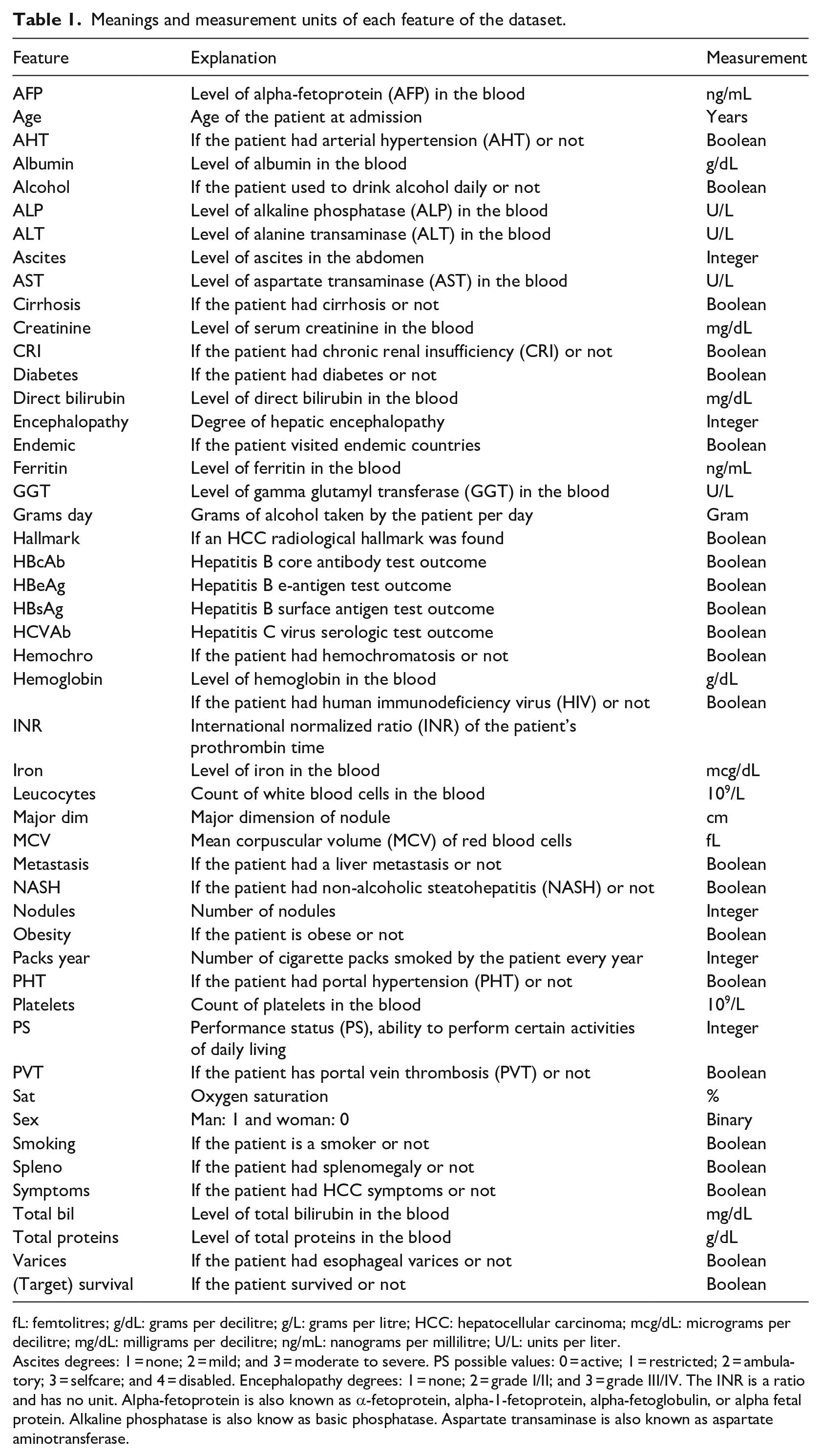
fL: femtolitres; g/dL: grams per decilitre; g/L: grams per litre; HCC: hepatocellular carcinoma; mcg/dL: micrograms per decilitre; mg/dL: milligrams per decilitre; ng/mL: nanograms per millilitre; U/L: units per liter.

Ascites degrees: 1 = none; 2 = mild; and 3 = moderate to severe. PS possible values: 0 = active; 1 = restricted; 2 = ambulatory; 3 = selfcare; and 4 = disabled. Encephalopathy degrees: 1 = none; 2 = grade I/II; and 3 = grade III/IV. The INR is a ratio and has no unit. Alpha-fetoprotein is also known as α-fetoprotein, alpha-1-fetoprotein, alpha-fetoglobulin, or alpha fetal protein. Alkaline phosphatase is also know as basic phosphatase. Aspartate transaminase is also known as aspartate aminotransferase.

A total of 24 clinical factors have binary values (Table 2), while 23 have real values or ordinal category values (Table 3). Most of the clinical features have missing values, with oxygen saturation (Sat) and Ferritin having the maximum percentage of 48.485% missingness (Table 3).

Table 2.

Statistical quantitative description of the binary features.

Binary feature	Value	#	%	Category feature	Value	#	%
AHT	0	103	62.424	Metastasis	0	125	75.758
AHT	1	59	35.758	Metastasis	1	36	21.818
AHT	Missing	3	1.818	Metastasis	Missing	4	2.424
Alcohol	0	43	26.061	NASH	0	135	81.818
Alcohol	1	122	73.939	NASH	1	8	4.848
Alcohol	Missing	0	0	NASH	Missing	22	13.333
Cirrhosis	0	16	9.697	Obesity	0	135	81.818
Cirrhosis	1	149	90.303	Obesity	1	20	12.121
Cirrhosis	Missing	0	0	Obesity	Missing	10	6.061
CRI	0	143	86.667	PHT	0	44	26.667
CRI	1	20	12.121	PHT	1	110	66.667
CRI	Missing	2	1.212	PHT	Missing	11	6.667
Diabetes	0	106	64.242	PVT	0	126	76.364
Diabetes	1	56	33.939	PVT	1	36	21.818
Diabetes	Missing	3	1.818	PVT	Missing	3	1.818
Endemic	0	116	70.303	Sex	0	32	19.394
Endemic	1	10	6.061	Sex	1	133	80.606
Endemic	Missing	39	23.636	Sex	Missing	0	0
Hallmark	0	52	31.515	Smoking	0	61	36.97
Hallmark	1	111	67.273	Smoking	1	63	38.182
Hallmark	Missing	2	1.212	Smoking	Missing	41	24.848
HBcAb	0	103	62.424	Spleno	0	66	40
HBcAb	1	38	23.03	Spleno	1	84	50.909
HBcAb	Missing	24	14.545	Spleno	Missing	15	9.091
HBeAg	0	125	75.758	(Target) survival	0	63	38.182
HBeAg	1	1	0.606	(Target) survival	1	102	61.818
HBeAg	Missing	39	23.636	(Target) survival	Missing	0	0
HBsAg	0	132	80	Symptoms	0	53	32.121
HBsAg	1	16	9.697	Symptoms	1	94	56.97
HBsAg	Missing	17	10.303	Symptoms	Missing	18	10.909
HCVAb	0	122	73.939	Varices	0	44	26.667
HCVAb	1	34	20.606	Varices	1	69	41.818
HCVAb	Missing	9	5.455	Varices	Missing	52	31.515
Hemochro	0	135	81.818
Hemochro	1	7	4.242
Hemochro	Missing	23	13.939
HIV	0	148	89.697
HIV	1	3	1.818
HIV	Missing	14	8.485

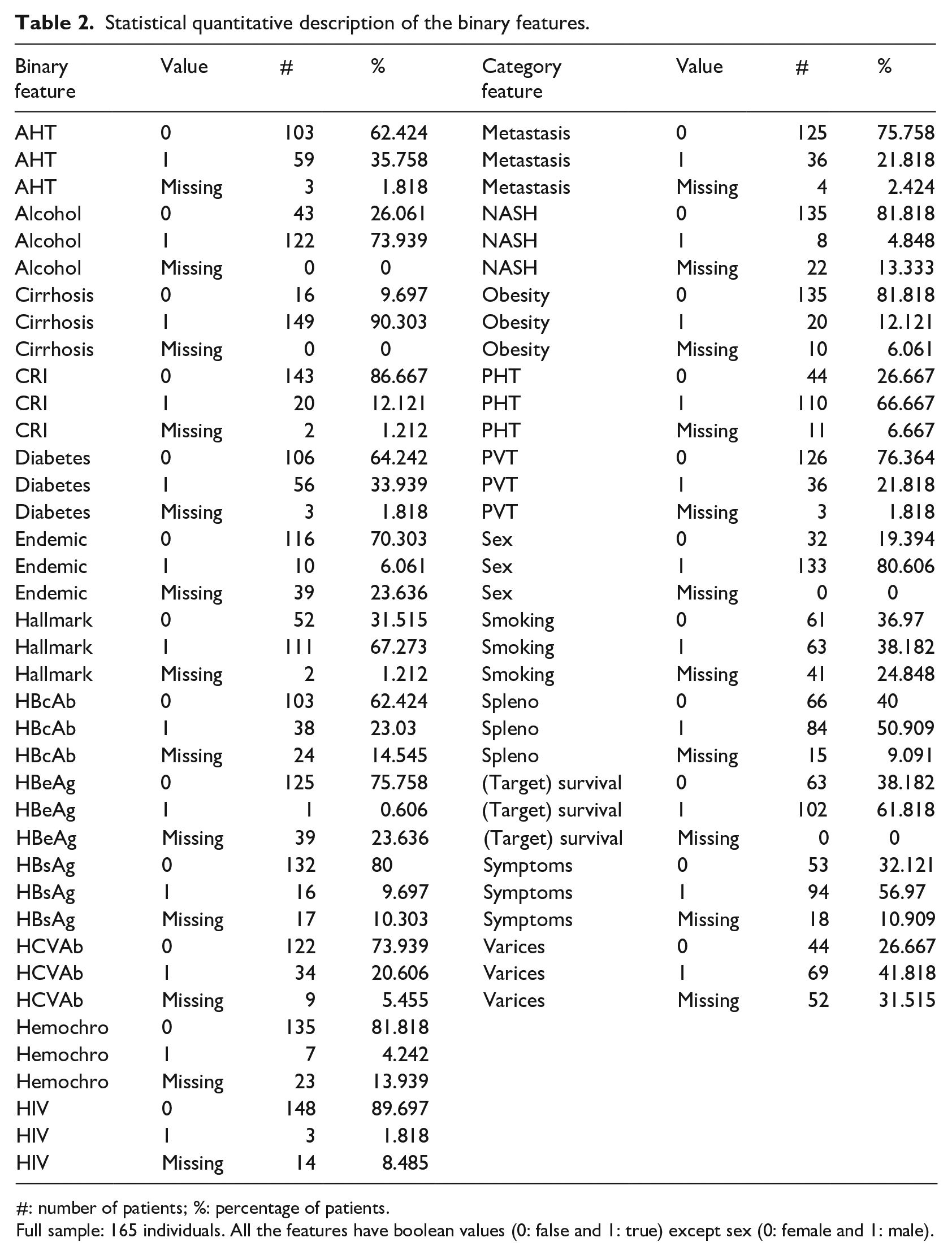
#: number of patients; %: percentage of patients.

Full sample: 165 individuals. All the features have boolean values (0: false and 1: true) except sex (0: female and 1: male).

Table 3.

Statistical quantitative description of the numeric features.

Numeric feature	Median	Mean	Range	σ	Missing #	Missing %
AFP	33.00	19,299.951	[1.2, 1,810,346]	149,098.336	8	4.848
Age	66.00	64.691	[20, 93]	13.320	0	0.000
Albumin	3.40	3.446	[1.9, 4.9]	0.685	6	3.636
ALP	162.00	212.212	[1.28, 98]	167.944	3	1.818
ALT	50.00	67.093	[11, 42]	57.540	4	2.424
Ascites	1.00	1.442	[1, 3]	0.686	2	1.212
AST	71.00	96.383	[17, 553]	87.484	3	1.818
Creatinine	0.850	1.127	[0.2, 7.6]	0.956	7	4.242
Dir bil	0.70	1.930	[0.1, 29.3]	4.210	44	26.667
Encephalopathy	1.000	1.159	[1, 3]	0.428	1	0.606
Ferritin	295.00	438.998	[0, 2230]	457.114	80	48.485
GGT	179.50	268.027	[23, 1575]	258.750	3	1.818
Grams day	75.00	71.009	[0, 500]	76.278	48	29.091
Hemoglobin	13.05	12.879	[5, 18.7]	2.145	3	1.818
INR	1.30	1.422	[0.84, 4.82]	0.478	4	2.424
Iron	83.00	85.599	[0, 224]	55.699	79	47.879
Leucocytes	7.20	1473.962	[2.2, 13,000]	2909.106	3	1.818
Major dim	5.00	6.851	[1.5, 22]	5.095	20	12.121
MCV	94.95	95.120	[69.5, 119.6]	8.406	3	1.818
Nodules	2.00	2.736	[0, 5]	1.798	2	1.212
Packs year	0.00	20.464	[0, 510]	51.565	53	32.121
Platelets	93,000.00	113,206.443	[1.71, 459,000]	107,118.632	3	1.818
PS	1.000	1.018	[0, 4]	1.182	0	0.000
Sat	27.000	37.029	[0, 126]	28.994	80	48.485
Total bil	1.400	3.088	[0.3, 40.5]	5.499	5	3.030
Total proteins	7.050	8.961	[3.9, 102]	11.729	11	6.667

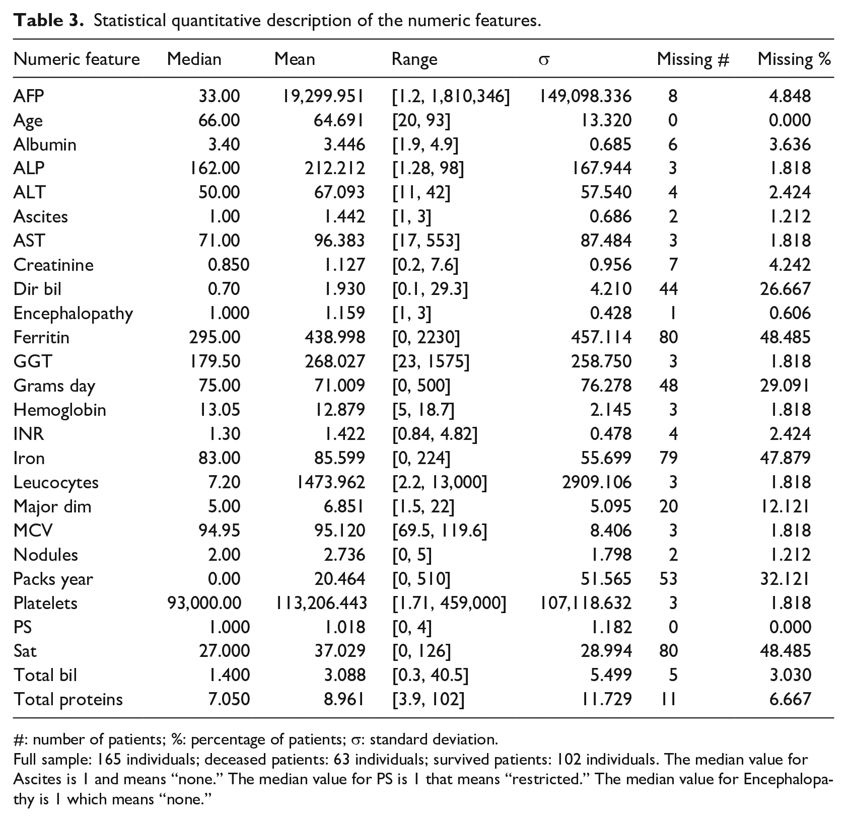
#: number of patients; %: percentage of patients; σ: standard deviation.

Full sample: 165 individuals; deceased patients: 63 individuals; survived patients: 102 individuals. The median value for Ascites is 1 and means “none.” The median value for PS is 1 that means “restricted.” The median value for Encephalopathy is 1 which means “none.”

The dataset is slightly imbalanced toward the positive class: there are 102 survived patients and 63 deceased patients, meaning 61.82% positive data instances and 38.18% negative data instances. The survival feature refers to 1 year after the hospital visit when the clinical data were recorded: if the patient profile has the positive survival label, it means she/he survived after 1 year; if the patient profile has a negative survival label, it means that she/he deceased within 1 year.

More information about this dataset can be found in the original publication by Santos et al.²⁷ and in the University of California Irvine Machine Learning Repository.²⁸

Methods

In this section we describe both the methods we used for binary classification and for feature ranking.

Let us consider the now-classical binary classification framework.^30,31 Let $X = X_{1} \times \dots \times X_{f}$ be the input space, consisting of $n_{f}$ features, and let $Y \in {0, 1}$ be the output space. Conventionally we will indicate with 1 a positive outcome and with 0 a negative outcome. Let $D_{n} = {(X_{1}, Y_{1}), \dots, (X_{n}, Y_{n})},$ where $X_{i} \in X$ and $Y_{i} \in Y$ $\forall i \in {1, \dots, n}$ , be a sequence of $n \in ℕ^{*}$ samples drawn independently from an unknown probability distribution µ over $X \times Y$ .

Before applying the classification and feature ranking algorithms, data must be pre-processed to be able to handle it and extract useful and actionable information (Data pre-processing and imputation). Let us consider a model (function) $f : X \to Y$ chosen from set F of possible hypotheses. An algorithm $A_{ℋ} : D_{n} \times ℱ \to f$ characterized by its hyper-parameters H selects a model inside a set of possible ones based on the available dataset, (section “Algorithms”). The error of f in approximating $ℙ {Y | X}$ is measured by a prescribed metric $M : ℱ \to ℝ$ . There are many different metrics available in literature for binary classification³² (Supplemental Material Information).

Note also that $D_{n}$ may be imbalanced (namely the $| {(X, Y) \in D_{n} : Y = 0} |$ may be ? or = than the $| {(X, Y) \in D_{n} : Y = 1} |$ ) and this may result in classifiers which produce unsatisfactory results on one of the two classes resulting in unsatisfactory metrics performance³³; for this reason we discuss the problem and show how we tackle it in this work (section “Handling unbalanced classes”). To tune the performance of the $A_{ℋ}$ , namely to select the best set of hyper-parameters, and to estimate the performance of the final model according to the desired metrics, a Model Selection (MS) and Error Estimation (EE) phase needs to be performed³⁴ (section “Model selection and error estimation”). Finally, we will also check for possible spurious correlations in the data by performing the Feature Ranking phase.³⁵

In fact, once the model is built based on the different learning algorithms and has been confirmed to be a sufficiently accurate representation of the $ℙ {Y | X}$ during the EE phase, one has to investigate how and how much the model is affected by different features that have been exploited to build the model itself during the feature ranking procedure (section “Feature ranking”).

Data pre-processing and imputation

Before employing a machine learning algorithm, data needs to be pre-processed.³⁶ In particular, $X_{i},$ with $i \in {1, \dots, n_{f}}$ , can be a categorical feature space (the values of the features belong to a finite unsorted set) or a numerical-valued feature space (the values of the features belong to a possibly infinite sorted set).

In the case of categorical feature space with more than two categories, if the algorithm is not able to handle multi-categorical features (for example, Support Vector Machines and Neural Networks), we will opt for the one hot encoding and we map it in a numerical feature space.³² Note also that some values of $X$ may be missing.³⁷

In this case, if the missing value is in a categorical feature, we introduce an additional category for missing values for that feature. If, instead, the missing value is associated with a numerical feature, we replace the missing value with the mean value of that feature and we introduce an additional logical feature to indicate whether the value of that feature is missing or not for a particular sample.

Algorithms

In this section we briefly recall the four algorithms that we have exploited in this study by pointing out the idea behind them, how to use them, and their hyper-parameters. The selected algorithms represent the most effective algorithms in four families of methods³¹: rule based methods, ensemble methods, kernel methods, and neural networks.

Decision Tree

A binary Decision Tree (DT)³⁸ belongs to the family of the rule based methods. The DT is a flowchart-like structure in which each internal node represents a test of a feature, each branch represents the outcome of the test, and each leaf node represents an output of the tree. A path from the root to a leaf represents a model rule.

A DT is built with a recursive schema until it reaches its desired depth d, which is the DT hyper-parameter that needs to be tuned during the MS phase. Each node of the DT, starting from the root node, is built by choosing the attribute and the cut that most effectively split the set of samples into two subsets based on the information gain.

The decision trees can handle categorical features, numerical features, and missing values well, and they do not suffer from numerical issues (no normalization of the data is needed).

Random Forests

The Random Forests (RF)³⁹ belong to the family of the ensemble methods. RF combine bagging to random subset feature selection. In bagging, each tree is independently constructed using a bootstrap sample of the dataset. RF add an additional layer of randomness to bagging. In addition to constructing each tree using a different bootstrap sample of the data, RF change how the classification trees are constructed.

In standard trees, each node is split using the best division among all variables. In a RF, each node is split using the best among a subset of predictors randomly chosen at that node. Eventually, a simple majority vote is taken for prediction. The accuracy of the final model depends mainly on three different factors: how many trees compose the forest, the accuracy of each tree and the correlation between them. The accuracy for RF converges to a limit as the number of trees $n_{t}$ in the forest increases, while it rises as the accuracy of each tree increases and the correlation between them decreases.

There are several hyper-parameters which characterize the performance of the final model: the number of trees, the number of samples to extract during the bootstrap procedure, the depth of each tree, the number of predictors exploited in each subset during the growth of each tree, and finally the weights assigned to each tree. Nevertheless, in common applications, the RF stability to these factors is quite low.³⁹

Since RF is basically a combination of many DTs, RF can handle categorical features, numerical features, and missing values well, and they do not suffer from numerical issues (no normalization of the data is needed).

Support Vector Machines

The Support Vector Machines (SVM)⁴⁰ belong to the family of the kernel methods.

Kernel methods are a family of techniques which exploits the “kernel trick” for distances to extend linear techniques to the solution of non-linear problems.⁴¹ Kernel methods select the model which minimizes the trade-off between the performance, measured with a defined metric (Supplemental Material Information), over the data and the complexity of the solution, measured with different measures of complexities.^31,40 Support Vector Machines (SVM), linear SVM (linear) and non-linear SVM (kernel), represent the most known and effective Kernel methods techniques.

The hyper-parameters of the SVM include the kernel, which is usually fixed and is the linear one for SVM (linear) and the Gaussian one for SVM (kernel),⁴² the kernel hyper-parameter $γ$ for SVM (kernel) and the regularization hyper-parameter $C$ . $C$ and $γ$ need to be tuned during the MS phase.

SVM cannot handle categorical features directly (therefore, the one hot encoding³² is needed) and they do suffer from numerical issues and consequently data must be re-scaled (in our case all the numerical features and targets have been scaled to have zero mean and variance equal to one).

Multi-Layer Perceptron Neural Network with Dropout

The Multilayer Perceptron Network with Dropout (MLP)^43,44 belongs to the family of the neural networks.

Neural networks are techniques which combine together many simple models of a human brain neuron, called perceptrons,⁴⁵ to build a complex network. The neurons are organized into stacked layers, connected together by weights that are learned based on the available data via back-propagation.⁴⁶

If the architecture of the neural network consists of only one hidden layer, it is called shallow, while, if multiple layers are staked together, the architecture is defined as deep. From a functional point of view both architectures have the same representation power⁴⁷ but in practice, for some applications like natural language processing and image analysis, deep networks outperform the shallow ones.^44,48

In our context, where the number of samples and features is limited, it is more reasonable to use a shallow network.^43,44 In particular, in this study, we exploited a well known and effective architecture, the MLP, where a single hidden layer is present, we train it with adaptive subgradient methods, and we tuned the following hyper-parameters during the MS phase⁴⁴: the number of neurons in the hidden layer $n_{h}$ , the dropout rate $p_{d}$ , the percentage of data to use as batch size $p_{b},$ the learning rate $r_{l}$ , the fraction of gradient to keep at each step $ρ$ , the learning rate decay $r_{d}$ , and the activation function.

The MLP, like SVM, fails to handle categorical features directly (consequently, the one hot encoding³² is needed) and they do suffer from numerical issues and consequently the data must be re-scaled (in our case we exploited the same re-scaling method exploited for SVM).

Handling unbalanced classes

Data available in bioinformatics for binary classification are often strongly unbalanced.^49–51 However, most learning algorithms work badly with imbalanced datasets and tend to perform poorly on the minority class and for these reasons several techniques have been developed to address this issue.³³

The first step toward the solution of this problem is to avoid applying the inappropriate evaluation metrics for model generated using imbalanced data.⁵² For example, overall accuracy is a very dangerous metric in this context since the more unbalanced is the dataset the more this metric tends to promote models which poorly perform on the minority class. For this reason, in this study we also included other metrics like Matthews correlation coefficient (MCC),⁵³ $F_{1}$ score, precision-recall area under the curve (PR AUC),⁵⁴ and receiver operating characteristic area under the curve (ROC AUC),⁵⁵ which are more suited for the case of imbalanced data (Supplemental Material Information). Since the MCC produces a high score only if the classifier is able to correctly predict the majority of positives and negatives, we focused on this statistical indicator and ranked our method performances according to it.^36,56 A high MCC, in fact, means high sensitivity, specificity, precision, and negative predictive value. A high value of other common rates such as $F_{1}$ score and accuracy, instead, do not guarantee them.

The second step toward the mitigation of the effects of having an unbalanced dataset is to modify the algorithm or the data, but currently the most practical and effective method involves the re-sampling of the data to synthesize a balanced dataset.³³ For this purpose we can under- or over-sample the dataset. Under-sampling balances the dataset by reducing the size of the abundant class. By keeping all samples in the rare class and randomly selecting an equal number of samples in the abundant class, a new balanced dataset can be retrieved for further modeling. Note that this method wastes a great deal of information (many samples may not be used). For this reason the oversampling strategy is more often exploited. It tries to balance the dataset by increasing the size of rare samples. Rather than removing abundant samples, artificial synthetized samples are generated (for example by repetition, by bootstrapping, or by synthetic minority). The latter method is the one that we exploited in this paper.

Model selection and error estimation

MS and EE deal with the problem of tuning and assessing the performance of a learning algorithm.³⁴ Resampling techniques like k-fold cross validation and non-parametric bootstrap are often used by practitioners because they work well in many situations.⁵⁷ Other alternatives exist, which represent foundations in the Statistical Learning Theory and give more insight into the learning process. Examples of methods in this last category include the seminal work of the Vapnik-Chervonenkis Dimension, its improvement with the Rademacher Complexity, the theory of compression, the Algorithmic Stability breakthrough, the PAC-Bayes theory, and more recently the Differential Privacy theory.³⁴

In this work we will exploit the resampling techniques which rely on a simple idea: the original dataset $D_{n}$ is resampled once or many ( $n_{r}$ ) times, with or without replacement, to build three independent datasets called learning, validation and test sets, respectively $ℒ_{l}^{r}$ , $V_{v}^{r}$ , and $T_{t}^{r}$ , with $r \in {1, \dots, n_{r}}$ . Note that $ℒ_{l}^{r} \cap V_{v}^{r} = ⊘$ , $ℒ_{l}^{r} \cap T_{t}^{r} = ⊘$ , $V_{v}^{r} \cap T_{t}^{r} = ⊘$ , and $ℒ_{l}^{r} \cup V_{v}^{r} \cup T_{t}^{r} = D_{n}$ for all $r \in {1, \dots, n_{r}}$ .

Then, to select the best combination of the hyper-parameters $ℋ$ in a set of possible ones $ℌ = {ℋ_{1}, ℋ_{2}, \dots}$ for the algorithm $A_{ℋ}$ or, in other words, to perform the MS phase, we needed to apply the following procedure:

ℋ^{*} : \arg \min_{ℋ \in ℌ} \sum_{r = 1}^{n_{r}} M (A_{ℋ} (ℒ_{l}^{r}), V_{v}^{r}),

(1)

where $A_{ℋ} (ℒ_{l}^{r})$ is a model built with the algorithm $A$ with its set of hyper-parameters $ℋ$ and with the data $ℒ_{l}^{r}$ and where $M (f, V_{v}^{r})$ is a desired metric. Since the data in $ℒ_{l}^{r}$ are independent from the ones in $V_{v}^{r}$ , the idea is that $ℋ^{*}$ should be the set of hyper-parameters which allows to achieve a small error on a data set, that is, independent from the training set.

Then, to evaluate the performance of the optimal model which is $f_{A}^{*} = A_{ℋ^{*}} (D_{n})$ or, in other words, to perform the EE phase, the following procedure has to be applied:

M (f_{A}^{*}) = \frac{1}{n_{r}} \sum_{r = 1}^{n_{r}} M (A_{ℋ^{*}} (ℒ_{l}^{r} \cup V_{v}^{r}), T_{t}^{r}) .

(2)

Since the data in $ℒ_{l}^{r} \cup V_{v}^{r}$ are independent from the ones in $T_{t}^{r}$ , $M (f_{A}^{*})$ is an unbiased estimator of the true performance, measured with the metric $M$ , of the final model.³⁴

If $n_{r} = 1$ , if $l$ , $v$ , and $t$ are aprioristically set such that $n = l + v + t$ , and if the resample procedure is performed without replacement, the hold out method is obtained.³⁴ For implementing the complete nested $k$ -fold cross validation, instead, it is needed to set $n_{r} \leq (\begin{matrix} n \\ k \end{matrix}) (\begin{matrix} n - \frac{n}{k} \\ k \end{matrix})$ , $l = (k - 2) \frac{n}{k},$ $v = \frac{n}{k}$ , and $t = \frac{n}{k}$ and the resampling must be done without replacement.⁵⁷ Finally, for implementing the nested non-parametric bootstrap, $l = n$ and $ℒ_{l}^{r}$ must be sampled with replacement from $D_{n},$ while $V_{v}^{r}$ and $T_{t}^{r}$ are sampled without replacement from the sample of $D_{n}$ that have not been sampled in $ℒ_{l}^{r}$ .⁵⁷ Note that for the bootstrap procedure $n_{r} \leq (\begin{matrix} 2 n - 1 \\ n \end{matrix})$ . In this study, we exploited the complete nested $k$ -fold cross validation because it represents the state-of-the-art approach.³⁴

Feature ranking

Once we built the models and they showed their effectiveness in predicting the desired quantities, we decided to investigate how these models are affected by the different features used in the model identification phase. We performed this operation to understand if the models also have a foundation which relies on the underlying phenomena or if the model just captures spurious correlations.³⁵

This procedure is called feature ranking (FR) and allows one to detect if the learned models appropriately take into account the relevant features. We consider relevant features the ones that are known to be important based on the literature or on the knowledge of the experts on the scientific problem.

The failure of the computational model to properly account for the relevant features might indicate poor quality in the measurements or spurious correlations. FR therefore represents an important step of model verification, since it should generate consistent results with the available knowledge of the phenomena under examination.

Since Random Forests was the method which obtained the best results in binary classification (Table 4), we took advantage of this ensemble learning technique to perform the feature ranking.

Table 4.

Results of the survival prediction made with machine learning classifiers.

Method	MCC	F₁ score	Accuracy	PR AUC	ROC AUC
RF	*+0.526 ± 0.011	*0.811 ± 0.005	*0.772 ± 0.005	0.149 ± 0.005	*0.766 ± 0.006
Linear SVM	+0.522 ± 0.011	*0.811 ± 0.005	0.771 ± 0.005	0.143 ± 0.005	0.763 ± 0.006
MLP	+0.456 ± 0.173	0.801 ± 0.090	0.727 ± 0.112	0.036 ± 0.044	0.695 ± 0.087
Radial SVM	+0.318 ± 0.130	0.744 ± 0.062	0.680 ± 0.065	0.191 ± 0.061	0.663 ± 0.068
DT	+0.295 ± 0.013	0.714 ± 0.006	0.659 ± 0.006	*0.211 ± 0.005	0.650 ± 0.006
Method	TP rate	TN rate	PPV	NPV
RF	0.794 ± 0.007	*0.738 ± 0.009	*0.829 ± 0.006	0.692 ± 0.009
Linear SVM	0.801 ± 0.007	0.724 ± 0.009	0.821 ± 0.006	0.697 ± 0.009
MLP	*0.950 ± 0.054	0.439 ± 0.174	0.705 ± 0.145	*0.836 ± 0.181
Radial SVM	0.729 ± 0.087	0.597 ± 0.087	0.765 ± 0.071	0.547 ± 0.127
DT	0.690 ± 0.008	0.610 ± 0.010	0.741 ± 0.007	0.549 ± 0.010

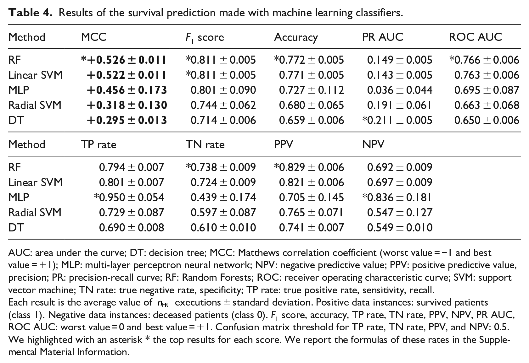
AUC: area under the curve; DT: decision tree; MCC: Matthews correlation coefficient (worst value = −1 and best value = +1); MLP: multi-layer perceptron neural network; NPV: negative predictive value; PPV: positive predictive value, precision; PR: precision-recall curve; RF: Random Forests; ROC: receiver operating characteristic curve; SVM: support vector machine; TN rate: true negative rate, specificity; TP rate: true positive rate, sensitivity, recall.

Each result is the average value of $n_{F R}$ executions ± standard deviation. Positive data instances: survived patients (class 1). Negative data instances: deceased patients (class 0). F₁ score, accuracy, TP rate, TN rate, PPV, NPV, PR AUC, ROC AUC: worst value = 0 and best value = +1. Confusion matrix threshold for TP rate, TN rate, PPV, and NPV: 0.5. We highlighted with an asterisk * the top results for each score. We report the formulas of these rates in the Supplemental Material Information.

Random Forests feature ranking

In this context, feature rankings methods based on Random Forests are among the most effective machine learning techniques,^58,59 particularly in the context of bioinformatics^60,61 and health informatics.¹⁹ Several measures are available for feature importance in Random Forests.

One approach is based on the Gini Importance or Mean Decrease in Impurity (MDI) which calculates each feature importance as the sum over the number of splits (across all trees) that include the feature, proportionally to the number of samples it splits.⁶² Another powerful approach is the one based on the Permutation Importance or Mean Decrease in Accuracy (MDA), where the algorithm assesses the importance for each feature by removing the association between that feature and the target.⁶² This goal can be achieved by randomly permuting⁶³ the values of the feature and measuring the resulting increase in error. The method also removes the influence of the correlated features.

In details, for every tree, two quantities are computed: the first one is the error on the out-of-bag samples as they are used during prediction, while the second one is the error on the out-of-bag samples after a random permutation of the values of a variable. These two values are then subtracted and the average of the result over all the trees in the ensemble is the raw importance score for the variable under examination. Both MDI and MDA can be adopted since they can be easily carried out during the main prediction process inexpensively.

Despite the effectiveness of MDI and MDA, when the number of samples is small, these methods might be unstable.^64–66 For this reason, in this study, instead of running the Feature Ranking (FR) procedure just once, analogously to what we have done for MS and EE, we sub-sample $D_{n}$ such that $S_{m} \subset D_{n}$ with $m = | S_{m} | = p_{FR} n$ , namely we randomly sample without replacement $100 \cdot p_{FR} %$ of the data in $D_{n}$ , we perform the $F R$ using $S_{m}$ and we repeat the procedure $n_{FR}$ times. The final rank of a feature will be the aggregation of the different ranking using the Borda’s method,⁶⁷ where we summed the two positions of each feature in the two rankings, and sorted the ranking accordingly.

Computational pipeline for binary classification and feature ranking

We can recap here the computation pipeline of the analysis with the following steps:

Construction of the dataset described earlier (Data pre-processing and imputation) and pre-process it;

We built a model with each of the algorithms described in Algorithms (DT, RF, SVM (linear), SVM (kernel), and NN). We will handle the unbalanced classes as described in Handling unbalanced classes. We will use the MS strategy described in Model selection and error estimation where we set the number of fold $k = 10$ . During the MS we searched the hyper-parameters using the following ranges

(a) DT: $ℋ = {d} \in {2, 4, 6, 8, 10, 12, 14,}$ ;

(b) RF: we set $n_{t} = 1000$ since increasing it does not increases the accuracy;

(d) SVM (kernel): $ℋ = {C, γ} \in ℛ \times ℛ$ ;

(e) NN: $\begin{array}{l} ℋ = {n_{h}, p_{d}, p_{b}, r_{l}, ρ, r_{d}} \in {5, 10, 20, 40, 80, 160} \times {0, 0.001, 0.01, 0.1} \times \\ {0.1, 1} \times {0.001, 0.01, 0.1, 1,} \times {0.9, 0.09} \times {0.001, 0.01, 0.1, 1} \end{array}$ and as activation function we used the rectified linear unit (ReLU)⁴⁴;

where $ℛ = {0.0001, 0.0005, 0.001, 0.005, 0.01, 0.05,$ $0.1, 0.5, 1, 5, 10, 50}$ ;

For each of the constructed models we reported the results using the EE strategy described in Model selection and error estimation and the confusion matrix metrics together with the standard deviation where we set $n_{r} = 100$ ;

We reported the ranking of the features selected by the two feature ranking procedures described in Feature ranking with $p_{FR} = 0.9$ and $n_{FR} = 1000$ .

Biostatistics univariate tests

After using machine learning for feature ranking, we decided to rank the features by using the results of univariate traditional statistical tests which statistically express the relationship between each clinical factor and survival.

As done by Patrício et al.²⁰ when analyzing health records of patients with breast cancer, we first applied the Shapiro–Wilk test⁶⁸ to each feature to check their distribution. Since the normality assumptions were unmet, we then applied the Mann–Whitney $U$ test to the real-valued features, the Kruskal–Wallis test to the category features, the chi-squared ( $χ^{2}$ ) test to the binary features, and ranked their $p$ -values.

The Mann–Whitney $U$ test (or Wilcoxon rank–sum test),⁶⁹ applied to each feature in relation to the survival target, states whether we can reject the null hypothesis that the distributions of the each feature for the two groups of samples defined by survival are the same. The Kruskal–Wallis test⁷⁰ is a variant of the Mann–Whitney $U$ test to use for ordinal category features.

The chi-squared test⁷¹ between two variables checks how likely an observed distribution is due to chance. The Mann–Whitney $U$ test should be employed for features with real values, while the chi-squared test should be employed for non-ordinal category features.

A low $p$ -value generated by these tests (close to 0) means that the analyzed feature strongly relates to survival, while a high $p$ -value (close to 1) means the there is no significant relationship. Once we obtained a $p$ -value for each feature, we ranked them from the lowest (highest correlation with survival) to the highest (lowest correlation with survival), generating a feature ranking for the real features and a feature ranking for the binary features.

Results

In this section, we first report and describe the binary classification results we obtained for the survival prediction (section “Survival prediction”), the feature ranking results we obtained through machine learning (section “Machine learning clinical feature ranking”), and the feature ranking results we obtained through traditional statistics tests (section “Biostatistics feature ranking”).

Survival prediction

We listed the survival prediction results in Table 4, by ranking them on the Matthews correlation coefficients.⁵³ We chose the MCC because it is the only confusion matrix score that generates a high score only if the classifier obtained a high score on the sensitivity, specificity, precision, and negative predictive value.^36,56

Our results show that all the methods were able to correctly predict most of the survived patients (positive data instances) and all the methods except MLP were capable of correctly precicting the majority of deceased patients (negative data instances), by obtaining MCC from +0.295 to +0.526 on average (Table 4). Random Forests outperformed all the other methods, by achieving the top MCC, $F_{1}$ score, accuracy, ROC AUC, specificity, and positive predictive value. Decision Tree performed better than the other algorithms regarding the precision-recall area under the curve (PR AUC); while the multi-layer perceptron neural network achieved the top sensitivity and negative predictive value.

All methods performed better on recall than on specificity, by obtaining an almost perfect true positive rate of 0.950 (MLP) as top recall and by attaining a top 0.738 true negative rate (RF). We believe this difference is caused by the dataset imbalance, since there are 38.18% negative data instances (deceased patients) and 61.82 positive data instances (survived patients). The high scores of precision and negative predictive value confirm the confidence of our survival prediction.⁷²

Our results show that the classifiers perform more efficiently when used to predict patients with high chance to decease (TP rate) than patients with high chance to survive (TN rate). This condition results being more advisable to us because, as we mentioned earlier, predicting patients more at risk of death is more urgent.

Machine learning clinical feature ranking

Since Random Forests obtained the best results classifying the survival target (Survival prediction), we decided to employ this method to detect the most predictive features, able to discriminate survived patients from deceased patients. We applied an ensemble learning feature ranking $n_{FR}$ times, each generating a ranking for the mean Gini purity decrease and a ranking for the mean accuracy decrease. We merged together the $n_{FR}$ Gini rankings and the $n_{FR}$ accuracy rankings through Borda’s method, and finally merged the two final rankings through the same technique.

The results showed ALP, AFP, Hemoglobin, Albumin, and Ferritin as top five clinical factors to distinguish survived patients from deceased patients in both the final Gini ranking and the final accuracy ranking. Regarding the features ranked in the last positions, instead, the two final rankings were discordant. Alcohol, Cirrhosis, Sex, Hallmark, and Obesity resulted being the less relevant factors in the merged ranking (Table 5).

Table 5.

Clinical feature ranking results.

Merged ranking position	Borda score	Clinical feature	Gini decrease final position	Gini decrease average position	Accuracy decrease final position	Accuracy decrease average position
1	2	ALP	1	1.3	1	1.5
2	4	AFP	2	1.7	2	1.9
3	6	Hemoglobin	3	3	3	3
4	8	Albumin	4	4.3	4	4.1
5	10	Ferritin	5	5.1	5	5
6	13	PS	7	7.6	6	6.4
7	14	AST	6	6	8	7.8
8	18	Symptoms	11	12	7	6.5
9	21	Platelets	10	10	11	11.2
10	22	Age	8	7.7	14	14.5
11	27	Total bil	14	14.8	13	14.1
12	28	Dir bil	19	17.6	9	9.3
13	29	GGT	9	9.3	20	20.5
14	33	Creatinine	15	15.5	18	20.3
15	34	INR	12	12.2	22	22.1
16	36	Ascites	26	25.3	10	10.9
17	37	Major dim	18	17.2	19	20.3
18	38	Iron	21	21.2	17	17.5
19	39	Hemochro	27	27.1	12	13.8
20	40	Leucocytes	13	13.1	27	26.4
21	41	Varices	25	24.9	16	15.4
22	43	MCV	17	16.4	26	25.9
23	43	Metastasis	28	28.1	15	14.6
24	44	Sat	23	22.7	21	20.7
25	44	Total proteins	16	15.6	28	26.9
26	46	Packs year	22	22.6	24	24.6
27	53	HBsAg	30	30.1	23	23.8
28	60	ALT	20	19.8	40	41
29	61	HCVAb	31	30.6	30	30.4
30	61	PVT	36	35.8	25	25.8
31	63	Nodules	29	29.5	34	34.3
32	64	Endemic	32	32.8	32	30.6
33	64	PHT	35	35.4	29	29.9
34	66	HBcAb	33	32.9	33	32.8
35	68	Grams day	24	24.5	44	42.3
36	70	Encephalopathy	39	39	31	30.4
37	73	Diabetes	38	37.8	35	37.5
38	77	AHT	40	40.5	37	38.7
39	77	HIV	41	41.1	36	37.5
40	81	Smoking	34	33.5	47	43.2
41	82	CRI	43	43.3	39	39.5
42	83	Spleno	37	36.5	46	42.5
43	84	HBeAg	46	45.5	38	39.5
44	85	NASH	42	42	43	42.2
45	89	Alcohol	47	46.5	42	42.1
46	90	Cirrhosis	49	49	41	41.7
47	93	Sex	48	48	45	42.4
48	93	Hallmark	44	43.5	49	46.6
49	93	Obesity	45	45.3	48	45.1

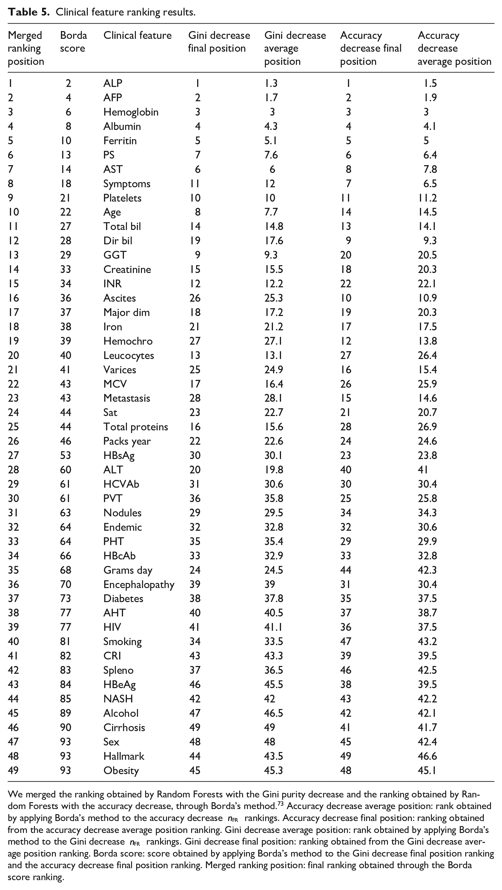
We merged the ranking obtained by Random Forests with the Gini purity decrease and the ranking obtained by Random Forests with the accuracy decrease, through Borda’s method.⁷³ Accuracy decrease average position: rank obtained by applying Borda’s method to the accuracy decrease $n_{F R}$ rankings. Accuracy decrease final position: ranking obtained from the accuracy decrease average position ranking. Gini decrease average position: rank obtained by applying Borda’s method to the Gini decrease $n_{F R}$ rankings. Gini decrease final position: ranking obtained from the Gini decrease average position ranking. Borda score: score obtained by applying Borda’s method to the Gini decrease final position ranking and the accuracy decrease final position ranking. Merged ranking position: final ranking obtained through the Borda score ranking.

As an example, we report a Gini ranking and an accuracy ranking generated by one of the applications of Random Forests out of $n_{FR}$ executions (Figure 1).

Figure 1.

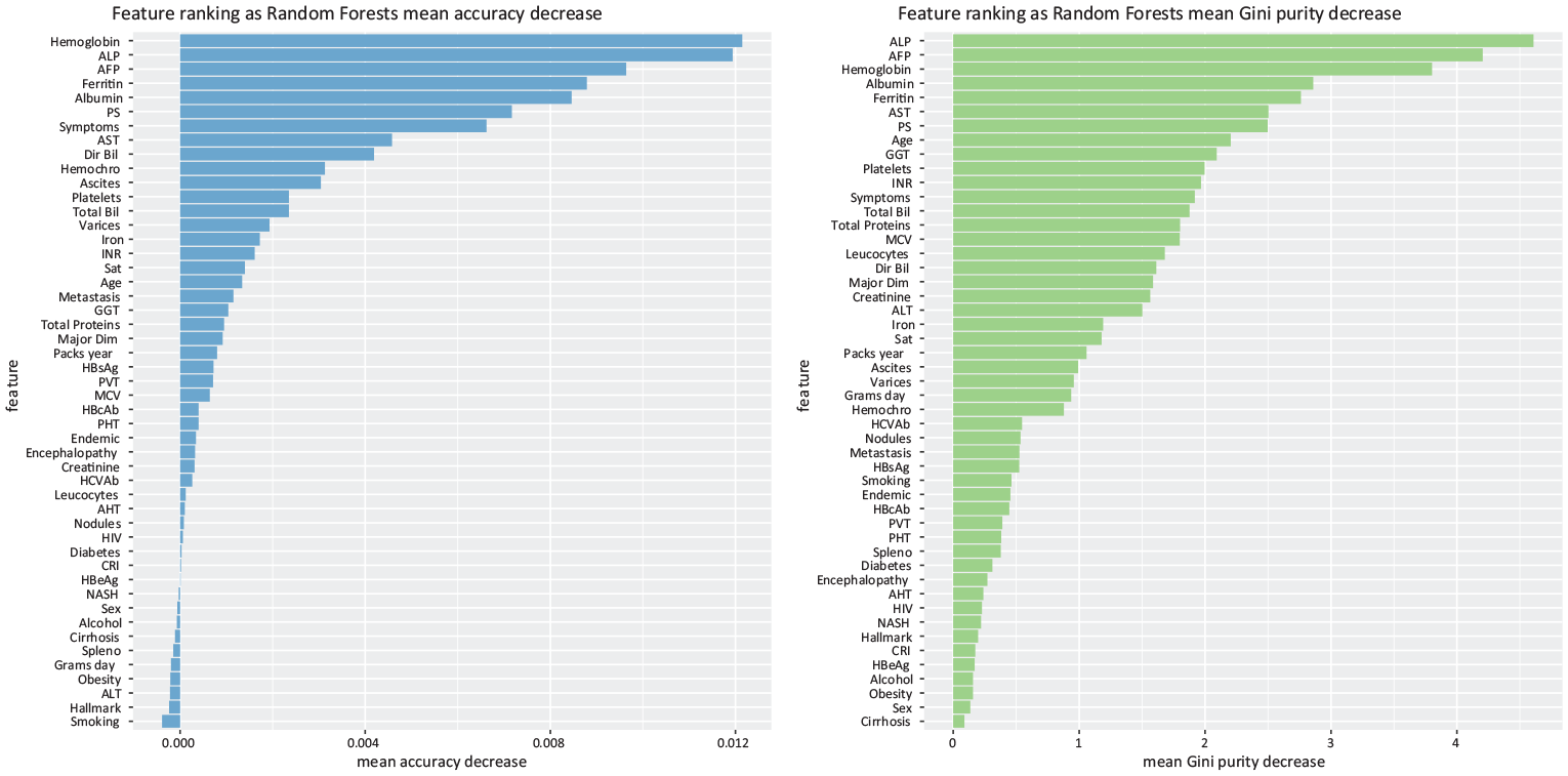
Random Forests feature selection. Indicative example of Random Forests feature selection through accuracy reduction (left) and Random Forests feature selection through Gini impurity (right), obtained in one of the $n_{F R}$ executions.

Biostatistics feature ranking

The Shapiro–Wilk test (Supplemental Table S1) produced a $p$ -values close to 0 for each feature, meaning that the null hypothesis of normality is rejected, and each variable distribution is non-normal.

We applied the Mann–Whitney $U$ test to the real-valued features, the chi-squared test to the binary features, and the Kruskall-Wallis test to the ordinal category features, all paired with survival, and then ranked the features according to their $p$ -values (Table 6). The tests’ results showed ALP, AFP, Hemoglobin, Direct Bilirubin (Dir Bil), AST, Ferritin, Symptoms, Metastasis, PS, Ascites as most significant features, having a $p$ -value lower than 0.005 (Table 6).

Table 6.

Results of the Mann–Whitney $U$ test applied to the real features (left), chi-squared test applied to the binary features (center), and Kruskal-Wallis test applied to the ordinal category features (right).

Position	Feature	Mann–Whitney $U$ test	Feature	Chi-squared test	Feature	Kruskal–Wallis test
Position	Feature	p-value	Feature	p-value	Feature	p-value
1	*ALP	$1.000 \times 10^{- 06}$	*Symptoms	$5.000 \times 10^{- 04}$	*PS	$2.000 \times 10^{- 06}$
2	*AFP	$4.000 \times 10^{- 06}$	*Metastasis	$4.498 \times 10^{- 03}$	*Ascites	$1.050 \times 10^{- 03}$
3	*Hemoglobin	$6.800 \times 10^{- 05}$	PVT	$1.050 \times 10^{- 02}$	Encephalopathy	$1.865 \times 10^{- 01}$
4	*Albumin	$2.100 \times 10^{- 04}$	HCVAb	$1.749 \times 10^{- 01}$	Nodules	$2.269 \times 10^{- 01}$
5	*Dir bil	$1.354 \times 10^{- 03}$	Diabetes	$1.769 \times 10^{- 01}$
6	*AST	$1.769 \times 10^{- 03}$	Endemic	$3.258 \times 10^{- 01}$
7	*Ferritin	$1.999 \times 10^{- 03}$	CRI	$3.283 \times 10^{- 01}$
8	Iron	$9.132 \times 10^{- 03}$	HBeAg	$3.818 \times 10^{- 01}$
9	GGT	$1.912 \times 10^{- 02}$	AHT	$4.138 \times 10^{- 01}$
10	Major dim	$2.816 \times 10^{- 02}$	Smoking	$4.543 \times 10^{- 01}$
11	INR	$3.298 \times 10^{- 02}$	Varices	$6.842 \times 10^{- 01}$
12	Total bil	$3.330 \times 10^{- 02}$	HBcAb	$6.867 \times 10^{- 01}$
13	Age	$3.568 \times 10^{- 02}$	Sex	$6.972 \times 10^{- 01}$
14	Creatinine	$9.698 \times 10^{- 02}$	Hemochro	$6.972 \times 10^{- 01}$
15	Platelets	$1.213 \times 10^{- 01}$	PHT	$6.992 \times 10^{- 01}$
16	Leucocytes	$1.405 \times 10^{- 01}$	NASH	$7.176 \times 10^{- 01}$
17	Total proteins	$1.514 \times 10^{- 01}$	Alcohol	$7.201 \times 10^{- 01}$
18	Sat	$3.319 \times 10^{- 01}$	Spleno	$7.421 \times 10^{- 01}$
19	Packs year	$3.940 \times 10^{- 01}$	Cirrhosis	$7.871 \times 10^{- 01}$
20	Grams day	$4.404 \times 10^{- 01}$	HBsAg	$7.906 \times 10^{- 01}$
21	MCV	$4.415 \times 10^{- 01}$	Obesity	$8.156 \times 10^{- 01}$
22	ALT	$6.641 \times 10^{- 01}$	Hallmark	$8.666 \times 10^{- 01}$
23			HIV	$1$

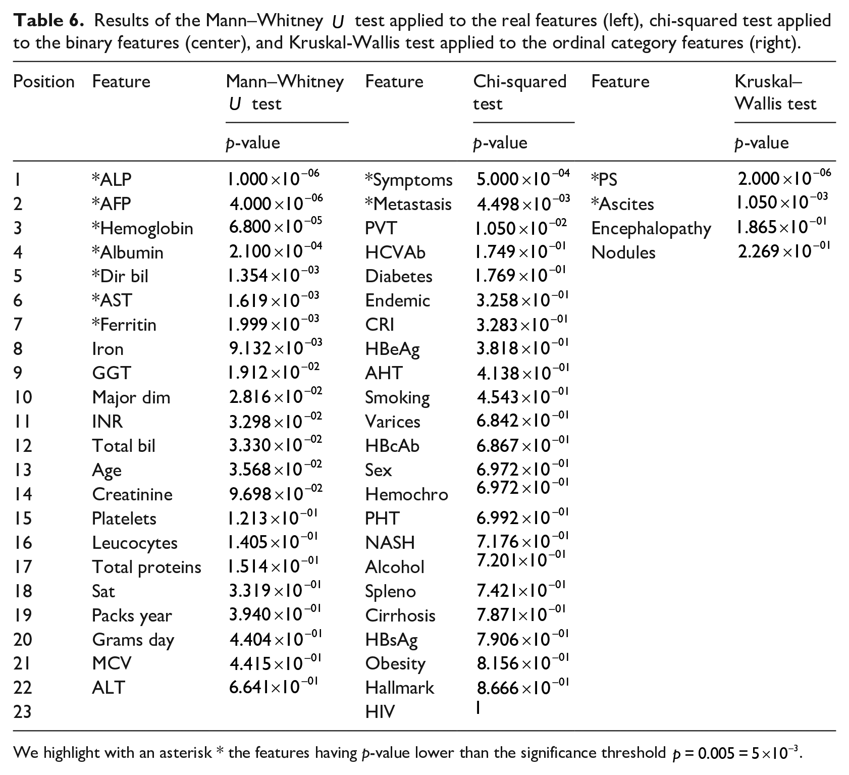
We highlight with an asterisk * the features having p-value lower than the significance threshold $p = 0.005 = 5 \times 10^{- 3}$ .

Exection times

We executed our scripts on a Dell Latitude 3540 personal computer running a Linux CentOS 7.10 operating system and R version 3.6. The execution of the binary classification methods took around 45 minutes, the exection of the feature ranking techniques took around 45 min and 30 s, while the execution of the biostatistics tests took around 5 seconds.

Discussion

In this section, we first discuss the results achieved by our binary classification for the survival prediction, and then we discuss the top predictive features detected by our computational intelligence approach, the top predictive features identified by our univariate statistical tests, and the top predictive features revealed by other studies.

Survival prediction

Our survival prediction results show that computational intelligence can effectively predict survival of patients from their clinical records, in few minutes and with small computational resources.

Our methods achieved good prediction results on all the confusion matrix rates (Survival prediction), and even outperformed the results obtained by the original dataset curators Santos et al.²⁷ which obtained a top performance score of ROC AUC = 0.700 through a neural network augmented sets approach. Our Random Forests classifier, in fact, obtained an average ROC AUC = 0.766 (Table 5). We believe that our improvement on the results, compared to the original study²⁷ is due mainly to the predictive power of Random Forests,³⁹ that often outperforms artificial neural networks and all the other machine learning techniques in health informatics binary classification tasks.^19,74–77

Other studies have applied machine learning methods to predict survival and rank the clinical features on this HCC dataset (Dataset), but they included methodological mistakes that led to inflated and overoptimistic results. Ksikazek et al.⁷⁸ obtained inflated prediction scores due to several wrong machine learning practices: they split the dataset into a training set and a test set, used the test set for the hyper-parameter optimization of their Genetic Algorithm, and then applied their trained model on the same test set, generating high predictive results. The correct practice necessitates to splitting the dataset into three separate subsets: training set, validation set, and test set.^34,36,43 The validation set should be employed for the hyper-parameter optimization, and the test set should be left untouched as a “held-out set” until the end, and used for the final classification made with trained optimized model.⁷⁹

In a parallel work, Sawhney et al.⁸⁰ committed a similar mistake: they decided to reduce the number of features of the dataset to predict survival, but they did it on the same subset they employed for testing their classification method. Again, the correct practice would have necessitated to splitting the dataset into three independent subsets: training set, feature reduction set, and test set. The “held-out” test set should have been used only at the end, after the training phase and the feature reduction phase. Additionally, the authors did not provide enough details on their feature reduction procedure.

Because of these malpractices, from a data analytics point of view, we did not compare our predictions performance with the results achieved by Ksikazek et al.⁷⁸ and Sawhney et al.⁸⁰ because the latter are biased and optimistic due to several data snooping issues (for example, some of the training data instances were employed also in the test set).⁸¹

Clinical feature ranking obtained by our Random Forests approach

Regarding feature ranking, our machine learning approach identified clinical factors already known to be HCC predictive or prognostic factors in the gastroenterology community (Table 6).

Yu et al.⁸² and Parikh and Sawant⁸³ for example, confirmed the predictive power of alkaline phosphatase (ALP) level for survival of patients having hepatocellular carcinoma. ALP is the top most predictive clinical factor found by our approach (Table 6). On the second position of our ranking we found alpha-fetoprotein (AFP), which was found to be strongly correlated to survival of patients having HCC by Tangkijvanich et al.,⁸⁴ Johnson,⁸⁵ Johnson and Williams,⁸⁶ and Tyson et al.,⁸⁷ in studies independent from each other. Finkelmeier et al.⁸⁸ confirmed the predictive importance of Hemoglobin level, which is on the third position of our ranking. The fourth position of our ranking lists the Albumin level, which has been confirmed to be related conditions of patients having hepatocellular carcinoma by Carr and Guerra⁸⁹ and Tanriverdi.⁹⁰

Regarding the Ferritin level found in the blood of patients, listed on fifth position of our ranking, the scientific literature contains several studies confirming this association.^91–93 However, since the Ferritin feature has almost half of its values missing in the the original dataset (Dataset), we have to warn that the data imputation technique we used might have influenced this outcome.

The fact that our approach ranked factors already known to the gastroenterology community as most predictive of survival for patients having HCC confirms the effectiveness of our feature ranking approach. Interestingly, our approach listed ALP level, AFP level, Hemoglobin level, and Ferritin level in positions higher than other known HCC clinical factors.

The last five positions of our ranking, in fact, list Alcohol consumption, Cirrhosis, Sex, Radiological Hallmark, and Obesity as least predictive features for HCC patient survival. Even if the daily consumption of alcohol is known to be related to to hepatocellular carcinoma,⁹⁴ our analysis suggests it is unrelated to survival. Regarding Cirrhosis, even if often present in patients with hepatocellular carcinoma,⁹⁵ our ranking recommends it as non-predictive of survival. A study by Sangiovanni et al.⁹⁶ confirms the increased chances of survival for patients with HCC and cirrhosis. Our analysis suggests that the patient’s sex is not prognostic of survival, even if HCC is more common among men. Even if the hepatocellular carcinoma diagnosis is confirmed by the Radiological Hallmark, our study states that this aspect cannot say anything about possible survival or decease of the patient. Obesity is a known risk factor for HCC,⁹⁷ but our study suggests, that is, independent from the survival of the patient.

Clinical feature ranking obtained by our univariate statistical tests

Regarding biostastistics univariate tests, we noticed these techniques identified as most relevant clinical factors the same top eight features found by Random Forests (ALP, AFP, Hemoglobin, Albumin, Ferritin, PS, AST, Symptoms), plus other ones that were on lowest Random Forests ranks. Our ensemble learning technique, in fact, put Direct Bilirubin on 12th position, Ascites on 16th position, and Metastasis on 23rd position out of 49.

Platelet count, Age, and Total Bilirubin result being more relevant than Direct Bilirubin in our machine learning ranking, confirming the effectiveness of Random Forests in this task. Platelet count, in fact, is a known prognostic factor in hepatocellular carcinoma,⁹⁸ but it was undetected as relevant feature by the univariate statistical tests (Table 6). Age is another important factor: older patients have less chance to survive HCC,⁹⁹ but Age was unseen as a key factor by the univariate statistical tests (Table 6).

Ascites is a prognostic factor employed by the Okuda HCC staging definition⁸ that was introduced in 1985 and by the Chinese University Prognostic Index¹³ in 2002, but was excluded from more common staging systems such as the TNM Classification of Malignant Tumors.^16,17

Metastasis was detected as a significant factor by the univariate statistical tests, but not by our Random Forests ranking.

HCC most predictive clinical features according to other studies

In the scientific literature, other papers claim alternative survival or mortality factors for HCC patients, which we compare with our top ranked features.

Cai et al.¹⁰⁰ listed tumor size and vascular invasion as the most relevant clinical features for survival of patients with hepatocellular carcinoma. The study of El-Fattah et al.¹⁰¹ instead, stated that age, race, tumor size, AFP level, the American Joint Committee on Cancer (AJCC) stage, and the year of diagnosis were the most relevant factors for survival in the medical records of HCC-diagnosed patients. Falkson et al.¹⁰² identified impaired performance status, male sex, older age, and disease symptoms (jaundice and reduced appetite) as factors most mortality-related. The research study of Vauthey et al.¹⁰³ identified cirrhosis and vascular invasion as clinical aspects more correlated to mortality.

Treatment for HCC, albumin level, and TNM stage were the most predictive survival features found by Kawaguchi et al.¹⁰⁴ in a recent article. Singal et al.¹⁰⁵ listed AFP and being a male as two relevant signs of potential survival from HCC. The article of Chaudhari et al.¹⁰⁶ instead, listed age, stage of disease, multiplicity, tumor thrombosis, lymphovascular invasion, nodal and distant metastases and completeness of resection as relevant factors for patients survival from HCC.

Two of these studies confirmed the relevance of AFP level,^101,105 which we ranked $2^{n d}$ in our analysis (Table 5), endorsing the predictive power of the $α$ -fetoprotein level in blood, that now can be considered a strong biomarker of survival from HCC.

Two studies listed male sex as a top predictive factor,^101,106 which we listed in the last positions of our ranking (Table 5): this discordance leaves room for further analysis about this aspect.

Conclusion

Hepatocellular carcinoma is a type of liver cancer that affects tens of millions of people worldwide (14 million in 2012¹) and kills approximately 800 thousand individuals worldwide every year.^2,3 Predicting survival and detecting the most relevant clinical features for patient survival can be extremely useful to better understand this disease and its medical markers.

In this context, machine learning can provide methods to analyze clinical records in a few minutes and suggest the most relevant clinical factors for survival. In this study, we analyzed a public dataset of medical data of 165 patients recorded in Coimbra (Portugal), which contain 50 features for each patient. We first applied a data imputation and oversampling approach to take care of the missing values and of the dataset imbalance. We then employed several data mining methods to discriminate the survived patients from the deceased patients, outperforming the classification results obtained by the original dataset curators Santos et al.²⁷ Afterwards, we took advantage of our top performing method (Random Forests) to rank all the clinical features based on their relevance in predicting survival, discovering that the most important features resulted were alkaline phosphatase, alpha-fetoprotein, Hemoglobin, Albumin, and Ferritin levels.

We found scientific publications confirming the association between these features and hepatocellular carcinoma, which confirmed the soundness of our approach. We also compared our top features with other prognostic factor combinations we found in the medical literature, and we noticed some studies which endorsed the role of alpha-fetoprotein. Our analysis therefore suggests the inclusion of alkaline phosphatase and Hemoglobin in any future HCC prognostic indexes.

Even if other studies confirmed the relevance of ALT and AFP in hepatocellular carcinoma survival our study lists them as the two most important variables for the first time. This discovery can have impact on clinical practice, suggesting physicians and medical doctors to focus on these two clinical factors of the blood tests.

Our methods can result particularly useful if employed in small hospitals or clinics where medical imaging techninques for CT scan or MRI are unavailable.

As a limitation, we admit that employing a single dataset from a single hospital has been a drawback in our study: if we had an alternative dataset from another site as a validation cohort, we could have used it to confirm our findings. Our results might not generalize well to other clinical records. We searched online for public alternative datasets of patients having hepatocellular carcinoma, but unfortunately we found none.

Another limitation of this study has been the absence of survival time in the dataset. If this feature were present in the dataset, we could have framed our analysis to understand how long a patient would have survived, through methods such as a stratified logistic regression.¹⁰⁷

In the future, we plan to expand our analysis by making a comparison between the speed, the resources employed, and the cost of making the decision employed by our computational intelligence approach and the same elements employed by medical doctors in a hospital settings. Unfortunately we did not have this information to perform this comparison in this study, but we hope to obtain it for the future.

Regarding future developments, we also plan to apply our approach to hepatocellular carcinoma data derived from high throughput sequencing technologies, such as transcriptomics data.¹⁰⁸

We also aim at applying our approach to datasets of patients having other diseases such as neuroblastoma,¹⁰⁹ breast cancer,²⁰ amyotrophic lateral sclerosis,¹¹⁰ and heart failure.¹⁰⁷

Supplemental Material

sj-pdf-1-jhi-10.1177_1460458220984205 – Supplemental material for Computational intelligence identifies alkaline phosphatase (ALP), alpha-fetoprotein (AFP), and hemoglobin levels as most predictive survival factors for hepatocellular carcinoma

Supplemental material, sj-pdf-1-jhi-10.1177_1460458220984205 for Computational intelligence identifies alkaline phosphatase (ALP), alpha-fetoprotein (AFP), and hemoglobin levels as most predictive survival factors for hepatocellular carcinoma by Davide Chicco and Luca Oneto in Health Informatics Journal

Footnotes

Abbreviations

Declaration of conflicting interests

The author(s) declared no potential conflicts of interest with respect to the research, authorship, and/or publication of this article.

Funding

The author(s) received no financial support for the research, authorship, and/or publication of this article.

ORCID iD

Davide Chicco

Data availability

The dataset used in this project is publicly available on (University of California Irvine Machine Learning Repository under its license at: https://archive.ics.uci.edu/ml/datasets/HCC+Survival). Our software code is publicly available under the GNU General Public License v3.0 at: ()

Supplemental material

Supplemental material for this article is available online.

References

Rawla

Sunkara

Muralidharan

, et al. Update in global trends and aetiology of hepatocellular carcinoma. Contemp Oncol (Pozn) 2018; 22(3): 141.

American Cancer Society. Key statistics about liver cancer, https://www.cancer.org/cancer/liver-cancer/about/what-is-key-statistics.html (accessed 10 March 2020).

Villanueva

Hepatocellular carcinoma. N Engl J Med 2019; 380(1): 1450–1462.

Leong

TYM

Leong

ASY

. Epidemiology and carcinogenesis of hepatocellular carcinoma. HPB (Oxford) 2005; 7(1): 5–15.

Ghouri

Mian

Rowe

JH.

Review of hepatocellular carcinoma: epidemiology, etiology, and carcinogenesis. J Carcinog 2017; 16: 1.

Kumar

Zhao

Wang

XW.

Molecular carcinogenesis of hepatocellular carcinoma and intrahepatic cholangiocarcinoma: one step closer to personalized medicine?

Cell Biosci 2011; 1(1): 5.

Raza

Sood

GK.

Hepatocellular carcinoma review: current treatment, and evidence-based medicine. World J Gastroenterol 2014; 20(15): 4115.

Okuda

Ohtsuki

Obata

, et al. Natural history of hepatocellular carcinoma and prognosis in relation to treatment study of 850 patients. Cancer 1985; 56(4): 918–928.

Cancer of the Liver Italian Program (CLIP) Investigators. A new prognostic system for hepatocellular carcinoma: a retrospective study of 435 patients. Hepatology 1998; 28(3): 751–755.

10.

Llovet

Brú

Bruix

. Prognosis of hepatocellular carcinoma: the BCLC staging classification. In: Seminars in liver disease, Hospital Clinic, University of Barcelona, Barcelona, Spain, 1999, vol. 19, pp. 329–338. Leipzig, Germany: Thieme Medical Publishers.

11.

Chevret

Trinchet

Mathieu

, et al. A new prognostic classification for predicting survival in patients with hepatocellular carcinoma. J Hepatol 1999; 31(1): 133–141.

12.

Vauthey

Lauwers

Esnaola

, et al. Simplified staging for hepatocellular carcinoma. J Clin Oncol 2002; 20(6): 1527–1536.

13.

Leung

Tang

Zee

, et al. Construction of the Chinese University Prognostic Index for hepatocellular carcinoma and comparison with the TNM staging system, the Okuda staging system, and the Cancer of the Liver Italian Program staging system: a study based on 926 patients. Cancer 2002; 94(6): 1760–1769.

14.

Kudo

Chung

Osaki

Prognostic staging system for hepatocellular carcinoma (CLIP score): its value and limitations, and a proposal for a new staging system, the Japan Integrated Staging Score (JIS score). J Gastroenterol 2003; 38(3): 207–215.

15.

Villa

Colantoni

Cammà

, et al. Estrogen receptor classification for hepatocellular carcinoma: comparison with clinical staging systems. J Clin Oncol 2003; 21(3): 441–446.

16.

Subramaniam

Kelley

Venook

AP.

A review of hepatocellular carcinoma (HCC) staging systems. Chin Clin Oncol 2013; 2(4): 33.

17.

National Cancer Institute. Cancer staging, https://www.cancer.gov/about-cancer/diagnosis-staging/staging (accessed 4 March 2020).

18.

Cammà

Cabibbo

Prognostic scores for hepatocellular carcinoma: none is the winner. Liver Int 2009; 29(4): 478.

19.

Chicco

Rovelli

Computational prediction of diagnosis and feature selection on mesothelioma patient health records. PLoS One 2019; 14(1): e0208737.

20.

Patrício

Pereira

Crisóstomo

, et al. Using Resistin, glucose, age and BMI to predict the presence of breast cancer. BMC Cancer 2018; 18(1): 29.

21.

Modi

Ghanchi

. A comparative analysis of feature selection methods and associated machine learning algorithms on Wisconsin breast cancer dataset (WBCD). In: Proceedings of ICT4SD 2015—the 2015 international conference on information and communications technology for sustainable development, Ahmedabad, India, 3–4 July 2015, pp. 215–224. Singapore: Springer.

22.

Gupta

Tran

Luo

, et al. Machine-learning prediction of cancer survival: a retrospective study using electronic administrative records and a cancer registry. BMJ Open 2014; 4(3): e004007.

23.

Tannus

Almeida-Carvalho

Loureiro-Matos

, et al. Evaluation of survival of patients with hepatocellular carcinoma: a comparative analysis of prognostic systems. PLoS One 2018; 13(4): e0194922.

24.

Gui

Dong

, et al. Identification of hepatocellular carcinoma–related genes with a machine learning and network analysis. J Comput Biol 2015; 22(1): 63–71.

25.

Qin

Forgues

, et al. Predicting hepatitis B virus-positive metastatic hepatocellular carcinomas using gene expression profiling and supervised machine learning. Nat Med 2003; 9(4): 416–423.

26.

Yim

Denman

Kwan

, et al. Tumor information extraction in radiology reports for hepatocellular carcinoma patients. AMIA Jt Summits Transl Sci Proc 2016; 2016: 455–464.

27.

Santos

Abreu

García-Laencina

, et al. A new cluster-based oversampling method for improving survival prediction of hepatocellular carcinoma patients. J Biomed Inform 2015; 58: 49–59.

28.

University of California Irvine Machine Learning Repository. HCC survival data set, https://archive.ics.uci.edu/ml/datasets/HCC+Survival (accessed 25 February 2020).

29.

European Association for the Study of the Liver. EASL–EORTC clinical practice guidelines: management of hepatocellular carcinoma. J Hepatol 2012; 56(4): 908–943.

30.

Vapnik

VN.

Statistical learning theory. New York City, New York: Wiley, 1998.

31.

Shalev-Shwartz

Ben-David

Understanding machine learning: from theory to algorithms. Cambridge, MA: Cambridge University Press, 2014.

32.

Aggarwal

CC.

Data mining: the textbook. Heidelberg, Germany: Springer, 2015.

33.

Haixiang

Yijing

Shang

, et al. Learning from class-imbalanced data: review of methods and applications. Expert Syst Appl 2017; 73: 220–239.

34.

Oneto

Model selection and error estimation in a nutshell. Berlin, Germany: Springer, 2020.

35.

Guyon

Elisseeff

An introduction to variable and feature selection. J Mach Learn Res 2003; 3: 1157–1182.

36.

Chicco

Ten quick tips for machine learning in computational biology. BioData Min 2017; 10(35): 1–17.

37.

Donders

ART

Van Der Heijden

Stijnen

, et al. A gentle introduction to imputation of missing values. J Clin Epidemiol 2006; 59(10): 1087–1091.

38.

Rokach

Maimon

OZ.

Data mining with decision trees: theory and applications, vol. 69. Singapore: World Scientific, 2008.

39.

Breiman

Random forests. Mach Learn 2001; 45(1): 5–32.

40.

Shawe-Taylor

Cristianini

Kernel methods for pattern analysis. Cambridge, MA: Cambridge University Press, 2004.

41.

Scholkopf

. The kernel trick for distances. In: Dietterich TG, Becker S and Ghahramani Z (eds.) Advances in neural information processing systems Cambridge, MA: MIT Press 2001.

42.

Keerthi

Lin

CJ.

Asymptotic behaviors of support vector machines with Gaussian kernel. Neural Comput 2003; 15(7): 1667–1689.

43.

Bishop

CM.

Neural networks for pattern recognition. Oxford: Oxford University Press, 1995.

44.

Goodfellow

Bengio

Courville

Deep learning. Cambridge, MA: MIT Press, 2016.

45.

Rosenblatt

The perceptron: a probabilistic model for information storage and organization in the brain. Psychol Rev 1958; 65(6): 386.

46.

Rumelhart

Hinton

Williams

RJ.

Learning representations by back-propagating errors. Cogn Model 1988; 5(3): 1.

47.

Cybenko

Approximation by superpositions of a sigmoidal function. Math Control Signals Syst MCSS 1989; 2(4): 303–314.

48.

LeCun

Bengio

Hinton

Deep learning. Nature 2015; 521(7553): 436–444.

49.

Kerr

KF.

Comments on the analysis of unbalanced microarray data. Bioinformatics 2009; 25(16): 2035–2041.

50.

Laza

Pavón

Reboiro-Jato

, et al. Evaluating the effect of unbalanced data in biomedical document classification. J Integr Bioinform 2011; 8(3): 105–117.

51.

Han

Kim

Park

. Unbalanced sample size effect on the genome-wide population differentiation studies. In: Proceedings of BIBMW 2010—the 2010 IEEE international conference on bioinformatics and biomedicine workshops, Hong Kong, 18–21 December 2010, pp. 347–352. Hong Kong IEEE.

52.

Garcia

EA.

Learning from imbalanced data. IEEE Trans Knowl Data Eng 2008; 9: 1263–1284.

53.

Matthews

BW.

Comparison of the predicted and observed secondary structure of T4 phage lysozyme. Biochim Biophys Acta 1975; 405(2): 442–451.

54.

Saito

Rehmsmeier

The precision-recall plot is more informative than the ROC plot when evaluating binary classifiers on imbalanced datasets. PLoS One 2015; 10(3): e0118432.

55.

Chicco

Masseroli

. A discrete optimization approach for SVD best truncation choice based on ROC curves. In: Proceedings of IEEE BIBE 2013—the 13th IEEE international conference on bioinformatics and bioengineering, Chania, Greece,10–13 November 2013, pp. 1–4. Chania, Greece: IEEE.

56.

Chicco

Jurman

The advantages of the Matthews correlation coefficient (MCC) over F1 score and accuracy in binary classification evaluation. BMC Genomics 2020; 21(1): 1–16.

57.

Kohavi

. A study of cross-validation and bootstrap for accuracy estimation and model selection. In: Proceedings of IJCAI 1995—the 1995 international joint conference on artificial intelligence, vol. 14, Montreal, Quebec, Canada, 20–25 August1995, pp. 1137–1145.

58.

Saeys

Abeel

Van De Peer

Robust feature selection using ensemble feature selection techniques. In: Proceedings of ECML PKDD 2008—the 2008 joint European conference on machine learning and knowledge discovery in databases, Antwerp, Belgium, 15–19 September 2008, pp. 313–325. Antwerp, Belgium: Springer.

59.

Genuer

Poggi

Tuleau-Malot

Variable selection using random forests. Pattern Recognit Lett 2010; 31(14): 2225–2236.

60.

Random forest for bioinformatics. In: Zhang C, Ma Y (eds) Ensemble machine learning. Boston, MA: Springer, 2012, pp. 1–18.

61.

Díaz-Uriarte

De Andres

SA.

Gene selection and classification of microarray data using random forest. BMC Bioinformatics 2006; 7(1): 3.

62.

Louppe

Wehenkel

Sutera

, et al. Understanding variable importances in forests of randomized trees. In: Burges C (ed.) Advances in neural information processing systems, 2013, pp. 431–439.

63.

Good

Permutation tests: a practical guide to resampling methods for testing hypotheses. Heidelberg, Germany: Springer Science & Business Media, 2013.

64.

Calle

Urrea

Letter to the editor: stability of random forest importance measures. Brief Bioinform 2010; 12(1): 86–89.

65.

Kursa

MB.

Robustness of random forest-based gene selection methods. BMC Bioinformatics 2014; 15(1): 8.

66.

Wang

Yang

Luo

An experimental study of the intrinsic stability of random forest variable importance measures. BMC Bioinformatics 2016; 17(1): 60.

67.

Sculley

. Rank aggregation for similar items. In: Proceedings of the 2007 SIAM international conference on data mining, Minneapolis, Minnesota, USA, 26–28 April 2007, pp. 587–592. Minneapolis, Minnesota, USA: Society for Industrial and Applied Mathematics (SIAM).

68.

Shapiro

Wilk

MB.

An analysis of variance test for normality (complete samples). Biometrika 1965; 52(3/4): 591–611.

69.

Mann

Whitney

DR.

On a test of whether one of two random variables is stochastically larger than the other. Ann Math Stat 1947(18): 50–60.

70.

Kruskal

Wallis

WA.

Use of ranks in one-criterion variance analysis. J Am Stat Assoc 1952; 47(260): 583–621.

71.

Pearson

K. X.

On the criterion that a given system of deviations from the probable in the case of a correlated system of variables is such that it can be reasonably supposed to have arisen from random sampling. Lond Edinb Dublin Philos Mag J Sci 1900; 50(302): 157–175.

72.

LaMorte WW. Screening for disease: positive and negative predictive value, http://sphweb.bumc.bu.edu/otlt/MPH-Modules/EP/EP713_Screening/EP713_Screening5.html (accessed 3 February 2020).

73.

Lansdowne

Woodward

BS.

Applying the Borda ranking method. Airf J Logist 1996; 20(2): 27–29.

74.

Vedomske

Brown

Harrison

. Random forests on ubiquitous data for heart failure 30-day readmissions prediction. In: Proceedings of ICMLA 2013—the 12th international conference on machine learning and applications, Miami, Florida, USA, 4–7 December 2013, vol. 2, pp. 415–421. Miami, Florida, USA: IEEE.

75.

Bellos

Papadopoulos

Rosso

, et al. Categorization of patients’ health status in COPD disease using a wearable platform and random forests methodology. In: Proceedings of BHI 2012—the 2012 IEEE EMBS international conference on biomedical and health informatics, Hong Kong, 5–7 January 2012, pp. 404–407. Hong Kong: IEEE.

76.

Karlsson

Boström

Handling sparsity with random forests when predicting adverse drug events from electronic health records. In: Proceedings of ICHI 2014—the 2014 IEEE international conference on healthcare informatics, Verona, Italy, 15–17 September 2014, pp. 17–22. Verona, Italy: IEEE.

77.

Lee

Patient-specific predictive modeling using random forests: an observational study for the critically ill. JMIR Med Inform 2017; 5(1): e3.

78.

Ksikazek

Abdar

Acharya

, et al. A novel machine learning approach for early detection of hepatocellular carcinoma patients. Cogn Syst Res 2019; 54: 116–127.

79.

Skocik

Collins

Callahan-Flintoft

, et al. I tried a bunch of things: the dangers of unexpected overfitting in classification. bioRxiv 2016; 078816: 1–8.

80.

Sawhney

Mathur

Shankar

. A firefly algorithm based wrapper-penalty feature selection method for cancer diagnosis. In: Proceedings of ICCSA 2018—the 2018 international conference on computational science and its applications, Melbourne, Victoria, Australia, 2–5 July 2018, pp. 438–449. Melbourne, Victoria, Australia: Springer.

81.

White

A reality check for data snooping. Econometrica 2000; 68(5): 1097–1126.

82.

Chan

Lee

, et al. Alkaline phosphatase: does it have a role in predicting hepatocellular carcinoma recurrence? J Gastrointest Surg 2011; 15(8): 1440–1449.

83.

Parikh

Sawant

Raised alkaline phosphatase levels can predict hepatocellular carcinoma in decompensated cirrhotic patients. J Clin Exp Hepatol 2015; 5: S63.

84.

Tangkijvanich

Anukulkarnkusol

Suwangool

, et al. Clinical characteristics and prognosis of hepatocellular carcinoma: analysis based on serum alpha-fetoprotein levels. J Clin Gastroenterol 2000; 31(4): 302–308.

85.

Johnson

PJ.

The role of serum alpha-fetoprotein estimation in the diagnosis and management of hepatocellular carcinoma. Clin Liver Dis 2001; 5(1): 145–159.

86.

Johnson

Williams

Serum alpha-fetoprotein estimations and doubling time in hepatocellular carcinoma: influence of therapy and possible value in early detection. J Natl Cancer Inst 1980; 64(6): 1329–1332.

87.

Tyson

Duan

Kramer

, et al. Level of α-fetoprotein predicts mortality among patients with hepatitis C-related hepatocellular carcinoma. Clin Gastroenterol Hepatol 2011; 9(11): 989–994.

88.

Finkelmeier

Bettinger

Köberle

, et al. Single measurement of hemoglobin predicts outcome of HCC patients. Med Oncol 2014; 31(1): 806.

89.

Carr

Guerra

Serum albumin levels in relation to tumor parameters in hepatocellular carcinoma patients. Int J Biol Markers 2017; 32(4): 391–396.

90.

Tanriverdi

A discussion of serum albumin level in advanced-stage hepatocellular carcinoma: a medical oncologist’s perspective. Med Oncol 2014; 31(11): 282.

91.

Facciorusso

Del Prete

Antonino

, et al. Serum ferritin as a new prognostic factor in hepatocellular carcinoma patients treated with radiofrequency ablation. J Gastroenterol Hepatol 2014; 29(11): 1905–1910.

92.

Nakano

Kumada

Sugiyama

, et al. Clinical significance of serum ferritin determination for hepatocellular carcinoma. Am J Gastroenterol 1984; 79(8): 623–627.

93.

Hann

HWL

Kim

London

, et al. Increased serum ferritin in chronic liver disease: a risk factor for primary hepatocellular carcinoma. Int J Cancer 1989; 43(3): 376–379.

94.

Morgan

Mandayam

Jamal

MM.

Alcohol and hepatocellular carcinoma. Gastroenterology 2004; 127(5): S87–S96.

95.

Oka

Kurioka

Kim

, et al. Prospective study of early detection of hepatocellular carcinoma in patients with cirrhosis. Hepatology 1990; 12(4): 680–687.

96.

Sangiovanni

Del Ninno

Fasani

, et al. Increased survival of cirrhotic patients with a hepatocellular carcinoma detected during surveillance. Gastroenterology 2004; 126(4): 1005–1014.

97.

Caldwell

Crespo

Kang

, et al. Obesity and hepatocellular carcinoma. Gastroenterology 2004; 127(5): S97–S103.

98.

Pang

Zhang

, et al. The prognostic value of platelet count in patients with hepatocellular carcinoma: a systematic review and meta-analysis. Medicine (Baltimore) 2015; 94(37): e1431.

99.

Lei

Chau

, et al. The effect of age on the long-term prognosis of patients with hepatocellular carcinoma after resection surgery: a propensity score matching analysis. Arch Surg 2012; 147(2): 137–144.

100.

Cai

Wang

, et al. Prognostic factors affecting postoperative survival of patients with solitary small hepatocellular carcinoma. Chin J Cancer 2016; 35(1): 80.

101.

El-Fattah

Aboelmagd

Elhamouly

Prognostic factors of hepatocellular carcinoma survival after radiofrequency ablation: a US population-based study. United European Gastroenterol J 2017; 5(2): 227–235.

102.

Falkson

Cnaan

Schutt

, et al. Prognostic factors for survival in hepatocellular carcinoma. Cancer Res 1988; 48(24 Part 1): 7314–7318.

103.

Vauthey

Klimstra

Franceschi

, et al. Factors affecting long-term outcome after hepatic resection for hepatocellular carcinoma. Am J Surg 1995; 169(1): 28–35.

104.

Kawaguchi

Tokushige

Hyogo

, et al. A data mining-based prognostic algorithm for NAFLD–related hepatoma patients: a nationwide study by the Japan study group of NAFLD. Sci Rep 2018; 8(1): 1–13.

105.

Singal

Mukherjee

Elmunzer

, et al. Machine learning algorithms outperform conventional regression models in predicting development of hepatocellular carcinoma. Am J Gastroenterol 2013; 108(11): 1723.

106.

Chaudhari

Khobragade

Bhandare

, et al. Management of fibrolamellar hepatocellular carcinoma. Chin Clin Oncol 2018; 7(5): 51.

107.

Chicco

Jurman

Machine learning can predict survival of patients with heart failure from serum creatinine and ejection fraction alone. BMC Med Inform Decis Mak 2020; 20(16): 1–16.

108.

Kaur

Dhall

Kumar

, et al. Identification of platform-independent diagnostic biomarker panel for hepatocellular carcinoma using large-scale transcriptomics data. Front Genet 2019; 10: 1306.

109.

Maggio

Chierici

Jurman

, et al. Distillation of the clinical algorithm improves prognosis by multi-task deep learning in high-risk Neuroblastoma. PLoS One 2018; 13(12): e0208924.

110.

Kueffner

Zach

Bronfeld

, et al. Stratification of amyotrophic lateral sclerosis patients: a crowdsourcing approach. Sci Rep 2019; 9(1): 1–14.

Supplementary Material

Please find the following supplemental material available below.

For Open Access articles published under a Creative Commons License, all supplemental material carries the same license as the article it is associated with.

For non-Open Access articles published, all supplemental material carries a non-exclusive license, and permission requests for re-use of supplemental material or any part of supplemental material shall be sent directly to the copyright owner as specified in the copyright notice associated with the article.

0.00 MB

0.17 MB

Computational intelligence identifies alkaline phosphatase (ALP),alpha-fetoprotein (AFP),and hemoglobin levels as most predictive survival factors for hepatocellular carcinoma

Abstract

Keywords

Introduction

Dataset

Methods

Data pre-processing and imputation

Algorithms

Decision Tree

Random Forests

Support Vector Machines

Multi-Layer Perceptron Neural Network with Dropout

Handling unbalanced classes

Model selection and error estimation

Feature ranking

Random Forests feature ranking

Computational pipeline for binary classification and feature ranking

Biostatistics univariate tests

Results

Survival prediction

Machine learning clinical feature ranking

Biostatistics feature ranking

Exection times

Discussion

Survival prediction

Clinical feature ranking obtained by our Random Forests approach

Clinical feature ranking obtained by our univariate statistical tests

HCC most predictive clinical features according to other studies

Conclusion

Supplemental Material

sj-pdf-1-jhi-10.1177_1460458220984205 – Supplemental material for Computational intelligence identifies alkaline phosphatase (ALP), alpha-fetoprotein (AFP), and hemoglobin levels as most predictive survival factors for hepatocellular carcinoma

Footnotes

Abbreviations

Declaration of conflicting interests

Funding

ORCID iD

Data availability

Supplemental material

References

Supplementary Material