Sage Journals: Discover world-class research

Abstract

The obesity epidemic progresses everywhere across the globe, and implementing frequent nationwide surveys to measure the percentage of obese population is costly. Conversely, country-level food sales information can be accessed inexpensively through different suppliers on a regular basis. This study applies a methodology to predict obesity prevalence at the country-level based on national sales of a small subset of food and beverage categories. Three machine learning algorithms for nonlinear regression were implemented using purchase and obesity prevalence data from 79 countries: support vector machines, random forests and extreme gradient boosting. The proposed method was validated in terms of both the absolute prediction error and the proportion of countries for which the obesity prevalence was predicted satisfactorily. We found that the most-relevant food category to predict obesity is baked goods and flours, followed by cheese and carbonated drinks.

Keywords

databases and data mining food sales machine learning obesity supervised learning

Introduction

Overweight and obesity are major risk factors for a number of chronic diseases, including diabetes, cardiovascular diseases and cancer. The global number of overweight people (including obese) rose from 857 million to 2.1 billion between 1980 and 2010,¹ and in countries with an overall low obesity prevalence, a double burden of obesity and undernutrition might be present.² Changes in the composition of traditional diets towards processed foods, together with a decrease in physical activity due to industrialisation³ have been identified as key components to explain the epidemic. Across countries, differences in obesity prevalence may be explained by the ‘dynamics of caloric ecosystems’: large-scale patterns related to systems of food production, distribution, consumption, food culture and traditions.⁴

Finding the relationship between food sales and obesity form first principles is a major challenge, lately questioned.⁵ Traditional regression approaches limit the analysis to a small set of predictors and impose assumptions of independence and linearity.⁶ These assumptions are almost certainly violated when modelling the effect of differences in national diets comprising highly correlated food categories. Here, instead, we consider a machine learning (ML) approach,⁷ which, in contrast to models derived from first principles, does not require the analyst to define a functional form of the model.

In addition to its contemporary popularity in different fields, ML is also receiving increasing attention from public health researchers. Examples include studies in alcohol abuse,^8,9 mortality risk in non-severe pneumonia,¹⁰ detection of hospital-acquired infections,¹¹ evaluation of dose-response in continuous treatment¹² and predictions of non-communicable diseases based on socio-demographic characteristics.¹³ In the discipline of obesity and nutrition, ML has been relied upon to predict the adherence to dietary recommendations from survey data,¹⁴ childhood obesity after the age of two using electronic health records prior to the second birthday,¹⁵ obesogenic environments for children,¹⁶ and the aggregation of metabolomics, lipidomics and other clinical data to model drug dose response.¹⁷

We believe that incorporating methods developed by the ML community into public health can help us to improve predictions and discover rich structures among the available data and therefore enhance our understanding of complex problems in public health, as well as to aid the design of new policies. In particular, and within the diet and obesity disciplines, the contributions of this work are (1) to apply an ensemble of ML methods to predict obesity prevalence exclusively from food sales data and (2) to identify the food categories that are most relevant in the prediction of obesity.

Methods

Data sources

The data used in this work came from two sources: (1) food and beverage sales data in 48 categories for 79 countries from the Euromonitor data set¹⁸ and (2) the percentage of obese adult population in these countries during 2008 estimated by Ng et al.¹ Table 1 shows the food categories included in the analysis.

Table 1.

Food categories available in the Euromonitor database.

Food group	Categories
Soft drinks	Bottled water, carbonates, concentrates, juice, sport and energy drinks.
Hot drinks	Coffee, tea and other hot drinks.
Alcoholic drinks	Beer, premixes, spirits and wine.
Packaged food	Baby food, baked goods, breakfast cereals, ice cream/frozen desserts, butter/margarine, edible oils, processed fruits/vegetables, processed meat/seafood, ready meals, rice/pasta, sauces/dressings, soup, spreads, savoury snacks and sweet snacks.
Confectionery	Chocolate, gum and sugar.
Dairy	Cheese, drinking milk, yoghurt and sour milk, and other dairy.
Fresh food	Eggs, meat, fish/seafood, nuts, pulses, starchy roots, sugar/sweeteners, fruits and vegetables.
Ingredients	Cocoa powder, fats/oils, flours, milk and emulsifiers.

We predicted obesity prevalence in 2008 using the average food sales data from 2006 to 2008 (Euromonitor). The reason to average over 3 years of food sales was made to reduce the effect of short-term fluctuations in sales as well as to allow for metabolic adaptation to changes in caloric intake.¹⁹

Euromonitor data are gathered with local industry collaboration and store checks. The absence of values for a given category corresponds to the lack of records for that category, possibly due to non-regulated sales or to an undeveloped market for such merchandise. The latter could be secondary to a lack of investment or to governmental regulation for the banning of specific products, such like alcohol in Muslim countries. The sales database used in this study had 3792 entries, of which 22 corresponded to absent values (0.58%). The product category and country of these 22 entries were as follows: alcoholic premixes (Vietnam, Pakistan, Uzbekistan, Azerbaijan, Algeria, Georgia, Tunisia and Saudi Arabia); wine (Pakistan and Saudi Arabia); spirits (Saudi Arabia); soup (Uzbekistan and Vietnam); ready meals (Kenya, Nigeria and Uzbekistan); sport drinks (Uzbekistan); concentrates (Peru, Uzbekistan, Bolivia, Ukraine and Belarus). These 22 entries were given value zero.

ML methods

First, an exploratory analysis of the data was performed using principal component analysis (PCA), a method for (linear) dimensionality reduction.^20,21 Within PCA, the components are ranked in terms of how much variability in the data they explain, that is, the first principal component is the direction, in the data space, in which most of the variance in the data is explained.

The relationship between obesity prevalence and food purchases at the national-level was assessed with a supervised learning approach, where food sales were the features (inputs) and the obesity prevalences were labels (outputs). This regression problem, given the number of predictors and entries, can be analysed using tree-based methods and support vector machines (SVMs). Other methods, such as deep learning, require a much larger sample size.²²

Among tree-based methods, we find decision trees, random forest (RF) and gradient boosting machines. In our work, RF and extreme gradient boosting (XGB) were compared. RF is a well-established method that aggregates decision trees in parallel using a random selection of predictors.²³ However, XGB works by training trees in a sequential way: each boosted tree is built after we learn from previous trees.²⁴

However, kernel-based methods, such as SVM, operate by assessing similarity between a test input and data points in the training set through a similarity function known as kernel. The hyperparameters of SVM are the penalty of error, kernel width and kernel type.

With respect to overfitting, it is known that the risk of overfitting increases with the capacity of models to adjust to specific training sets.²⁵ Our results were obtained finding the optimal model parameters using grid-search minimisation of the mean square error (MSE), using 10-fold cross-validation. In other words, the parameters in the models were found using 10 different training sets, thus ensuring robustness to overfitting. In addition, our results also provide performance indices (root mean square error (RMSE)) over out-of-sample data; these figures validate the correct fit of the model.

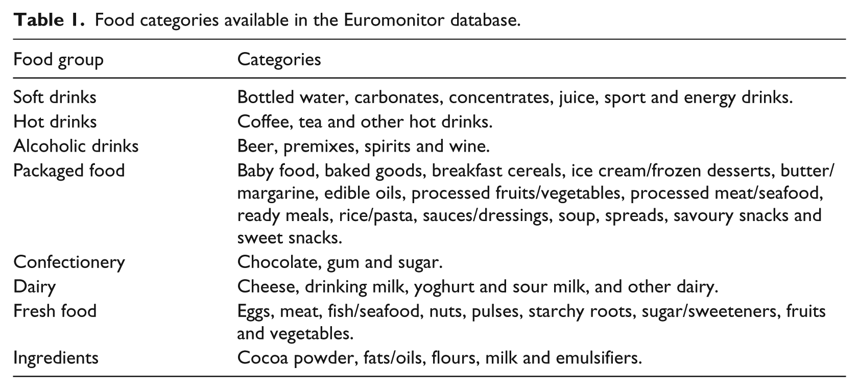
Figure 1 shows an example of a regression tree built choosing randomly from the available predictors with a maximum depth of two. In this case, the category flour is chosen and compared against a threshold of 17.8 kg per capita to identify groups of low versus high obesity. Then, each branch is further divided using the categories of sugar and cheese (with thresholds of 2.4 and 1.98 kg per capita, respectively). For this tree, the four terminal nodes (or leaves) have the following average prevalence for obesity: 0.065, 0.172, 0.174 and 0.236. For instance, a country that has a flour and cheese per capita intake greater than 17.8 and 1.98 kg, respectively, is predicted to have an obesity prevalence of 0.236.

Figure 1.

Example of regression tree with maximum depth of two, and that can use all the 48 categories to make the splits.

Free parameters of RF, XGB and SVM can be found in the Supplemental Appendix and the Python script developed for this work.

Results

Exploratory analysis

Sales within food and beverage group categories are summarised in Table 2, showing minimum, maximum and median for each food group. To address if sales distributions were normal, the Shapiro–Wilk test was applied, and asterisks indicate that the null hypothesis for normal distribution can be rejected. Summary statistics for each of the 52 food and beverages categories can be found in Table A1 in Supplemental Appendix.

Table 2.

Summary statistics for the food and beverage groups described in Table 1.

Food group (units) per capita per year	Minimum; maximum; median sales (Shapiro–Wilk test*)
Soft drinks (L)	3.59; 354.05; 117.80
Hot drinks (kg)	0.29; 10.76; 3.02*
Alcoholic drinks (L)	0.08; 185.90; 67.51*
Packaged food (kg)	7.40; 243.13; 130.99
Confectionery (kg)	0.16; 14.68; 3.57*
Dairy (kg)	0.63; 198.49; 57.00*
Fresh food (kg)	21.88; 400.44; 260.28
Ingredients (kg)	6.30; 256.43; 123.81*

p value < 0.05 (rejection of normal distribution hypothesis).

Relations between predictors were analysed using Spearman correlation test. With a threshold of 0.9, three pairs of highly correlated food categories were found: flours as ingredient and baked goods (0.98), milk as ingredient and drinking milk products (0.97), and emulsifiers with chocolate confectionery (0.90). These correlated food categories were replaced each one by the average value of the pair, ending in this way with 45 predictors.

The food purchase data were first explored using PCA, a dimensionality-reduction method that explains the variability of the observations. Figure 2(a) shows the cumulative proportion of variance explained as a function of the number of principal components. We found that the first 10 components explained 81 per cent of the data variation and that 50 per cent of the variance is explained using just the first two components. Focusing on these first two components, Figure 2(b) shows countries colour-coded according to their obesity prevalence and with different symbols for different continents.

Figure 2.

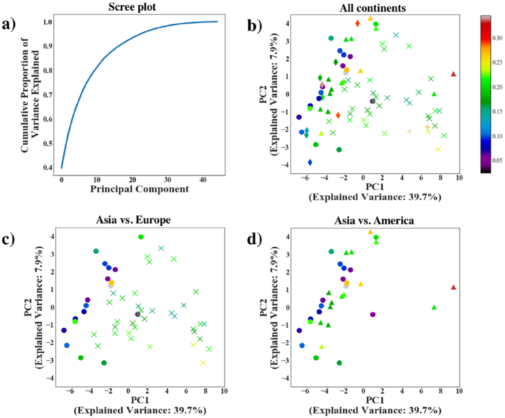
Principal component analysis of the food sales data: (a) screen plot for the proportion of variance explained as a function of the components; (b) first two principal components where each symbol corresponds to a country, colour-coded according to their obesity prevalence using a colourmap: Asia (disc), Africa (diamond), the Americas (triangle), Europe (x) and Oceania (+); (c) Asia and Europe only; and (d) Asia and America compared.

To visually explore the relation between diet components and geographical location, Figure 2(c) and (d) compares pairs of continents. Figure 2(c) displays the first two principal components for Asia and Europe, showing Asia with discs close together in the left side of the plot, as opposed to the ‘x’ representing Europe. These results show that obesity prevalence in Asia is smaller than in Europe, and that country prevalence is similar among countries within the same continent, especially in Europe. Conversely, Figure 2(d) displays results for Asia and America, showing similar first components for both continents, and therefore similar diet, except for the United States and Canada, which are represented by triangles on the far right side of the plot.

Predicting obesity from food: performance comparison

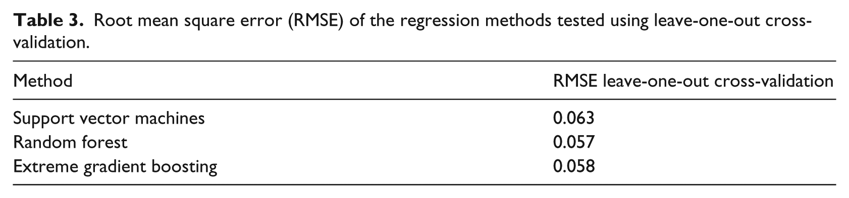
All the aforementioned regression methods were implemented using leave-one-out cross-validation (LOOCV) to predict one country’s obesity prevalence from the other 78 countries in the data set. Table 3 shows the RMSE for the three methods tested, finding that RF shows the best performance, closely followed by XGB.

Table 3.

Root mean square error (RMSE) of the regression methods tested using leave-one-out cross-validation.

Method	RMSE leave-one-out cross-validation
Support vector machines	0.063
Random forest	0.057
Extreme gradient boosting	0.058

Feature selection: variable importance list

Multiple trees’ average improves the predictive power of a single decision tree at the expense of interpretation loss. Nevertheless, the variable importance list (VIL) can give insights into the regression process by ranking food categories in terms of how much the RMSE changes when each category is removed.²³ A variable with a large importance means a significant increase in the error when such category is not used as a predictor.

From the algorithms tested here, RF and XGB offer the option of obtaining a VIL directly from the model. From the way these methods work, the ranking of variable importance is not necessarily the same: in RF, each tree is decorrelated and the learning process is done in parallel,²⁶ while in XGB, the boosting procedure implies that correlated variables are used only once in a given tree.²⁴ XGB is a more recent algorithm and there is ongoing discussion about the robustness of its VIL. Figure 3 shows the VIL obtained using RF, which was averaged over 250 runs.

Figure 3.

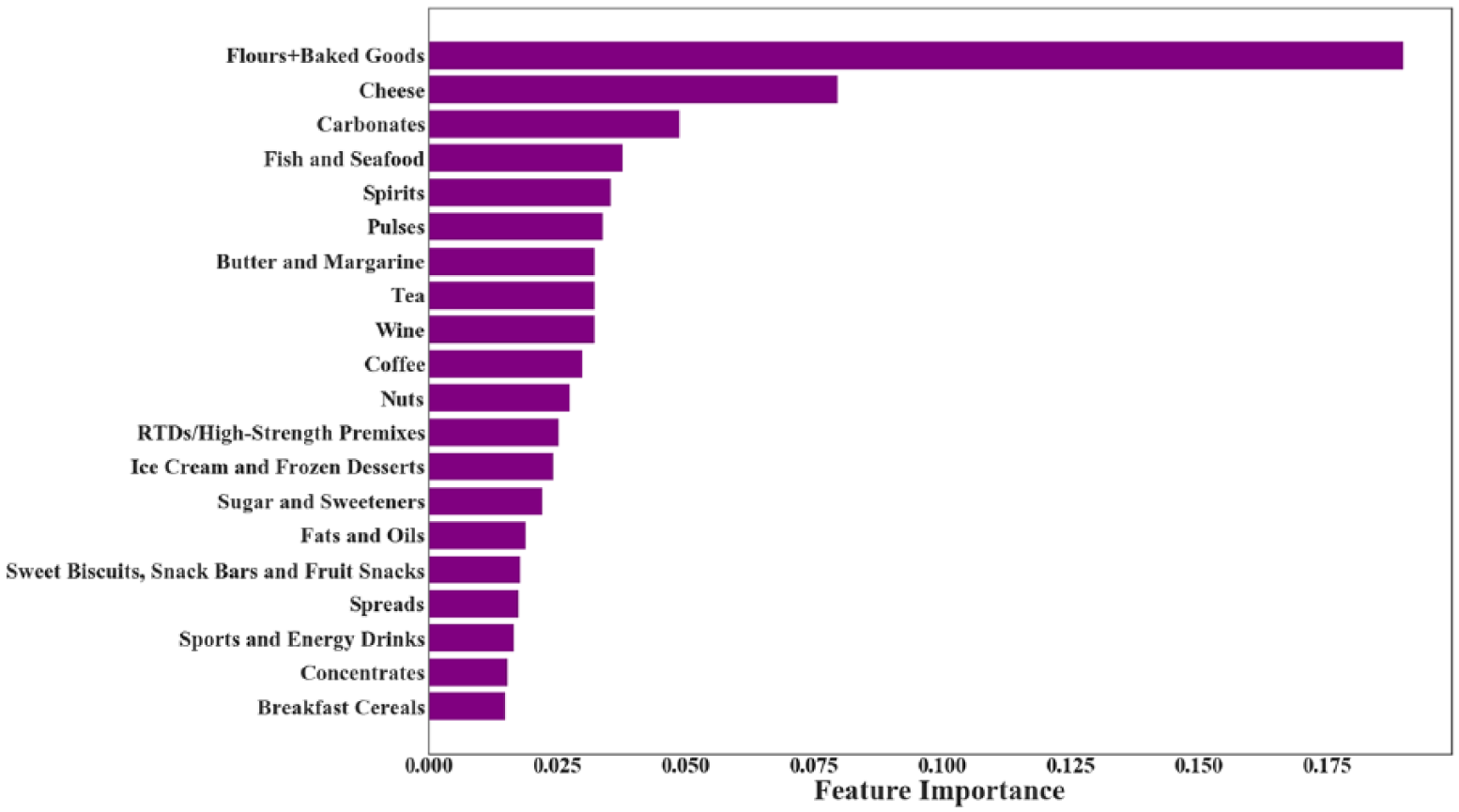
Averaged variable importance list for the first top 20 categories using RF.

We found that baked goods/flours was the best predictor of obesity prevalence, followed by cheese and later by carbonated drinks with less than half the importance of the best predictor. This VIL suggests that relative importance rapidly decreases as we move down the list. To assess whether we can limit our consideration to a smaller set of variables, we repeated the calculations using RF with only the top 5, 10, 15 and 20 categories from this list.

Prediction error using a subset of variables

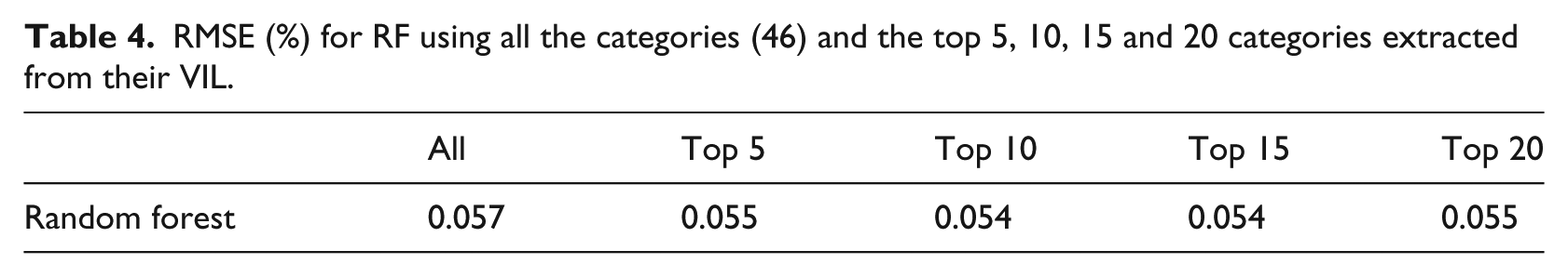
Table 4 compares the RMSE when RF uses all the categories, and when the top 5, 10, 15, and 20 categories are used instead. The parameters used to make these predictions were the ones obtained by grid-search (see the Supplemental Appendix), but with the maximum number of features manually constrained to these 5, 10, 15 and 20 categories, respectively. The prediction error slightly reduces when fewer variables were considered, which suggests that the consumption of some food categories may be associated with low obesity rates in certain countries, while in others, it is a predictor of high obesity prevalence.

Table 4.

RMSE (%) for RF using all the categories (46) and the top 5, 10, 15 and 20 categories extracted from their VIL.

	All	Top 5	Top 10	Top 15	Top 20
Random forest	0.057	0.055	0.054	0.054	0.055

Comparison between predicted and real values for obesity prevalence

To assess the predictive power of the model proposed in this study, we examined the distribution of the absolute prevalence prediction errors (APPEs), that is, the absolute difference between the predicted prevalence and true prevalence value. Since the maximum value of country obesity prevalence was 35 per cent for the countries analysed (equivalent to 0.35), we analysed the distribution of APPE by factors of 0.035, equivalent to 10 per cent error each.

Figure 4 shows the APPEs by number of countries analysed. The y-axis corresponds to APPEs, denoting 10, 20, 30 and 40 per cent errors of prediction. Of the total sample of countries, near 60 per cent of countries’ obesity prevalence was predicted with 10 per cent error or less, and 87 per cent of countries’ obesity prevalence with up to 20 per cent error. Countries with largest prediction errors were the United States, Uzbekistan, Georgia, Slovenia, Venezuela and Argentina.

Figure 4.

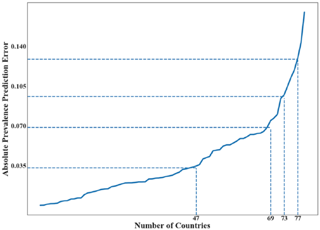
Absolute prevalence prediction error (APPE) using RF with the top five categories from the VIL. The countries are ordered according to their APPE, and the labels in the vertical axis indicate if the APPE is below 10, 20, 30 and 40 per cent of the of the full prevalence range [0, 0.35]. Notice that the obesity prevalence in 47 countries was predicted with less than 10 per cent error.

Discussion

We have proposed and applied a methodology to predict country-level obesity prevalence using food and beverage sales information. Our simulations confirm that RF, using only five categories, could predict obesity prevalence with an absolute error below 10 per cent (with respect to the entire prevalence range) for about 60 per cent of the countries considered, and below 20 per cent for 87 per cent of countries.

Recall that the relevance of the input variables to predict obesity is referred to as VIL, and this list allowed us to implement variants of the proposed methodology, but only using the 5, 10, 15 and 20 most-relevant food categories. These restricted methods provide estimates that are close to the unrestricted predictor (using all categories), but with a performance that is not necessarily monotonically increasing with the number of categories considered. This provided us with the following insight: first, nationwide obesity can be predicted only from a few food categories, and, second, the role of some categories (with a low VIL rank) might be contradictory, meaning that they increase obesity in some countries, but decrease obesity in others, and therefore, they lower the performance of the algorithm when included.

The top three categories in predicting country-level obesity were baked goods/flours, cheese and carbonated drinks. This list is in agreement with research that has identified processed foods as key drivers of the obesity epidemic.^27–29 Simple carbohydrates, for example, have been linked to the development of adiposity due to their high glycaemic load³⁰ and low fiber content.³¹ Cheese, however, is high in calories, fat and salt, and in most countries, a highly processed product. The third place is occupied by carbonated drinks, consumption of which has been associated with increased obesity risk in diverse populations, and clearly, it is not part of traditional diets.^32–35

We were not able to determine whether the change in national diet composition is a true cause of higher obesity prevalence or a surrogate marker of the concomitant rise in sedentary behaviour. However, previous research has hypothesised that the obesity epidemic is predominantly driven by the foods that are consumed and not by changes in caloric expenditure.^36,37

This study used ML methods and its results need to be interpreted considering both their strengths and limitations. While it is possible to establish the relative ranking of different national diet components for the overall predicting accuracy, this does not support the idea of independent risk factors; for instance, a society that reduces its consumption of cheese will see a reduction in obesity rates per se. Our goal was to identify food sales that could provide us with information about the synergic roles of categories. We used aggregate data to characterise both the exposure (composition of country-level food sales) and the outcome (country-level obesity prevalence). This also is a strength and a limitation. Our analysis cannot be used to claim that an individual living in a country with a given national diet is at elevated risk of high obesity prevalence. However, the application of ML to sales data has allowed us to estimate country-level obesity from five foods’ sales categories, a method that is less costly than national surveys.³⁸

Here, we considered food sales per capita instead of food consumption. In this regard, food waste is an important issue and has been reported to differ by food category, with diary and fresh foods being discarded in greater amounts than processed foods are,³⁹ and positively correlated with per capita gross domestic production.⁴⁰ It is important to note that sales data analysed here include food consumed by children, which are not considered in the obesity prevalence (calculated for adults older than 20 years). Finally, the data are obtained from industry data that aggregate 79 countries, where most low-income countries were excluded. In other words, the results presented here were obtained using mostly sales data from high- and upper-middle-income countries, and therefore, the conclusions drawn cannot be generalised to all countries.

Another limitation of this study is the use of available sales data registered by local industry and store checks based on the regulated market. These data do not allow for the estimation of the role of non-official sales in the prevalence of obesity. While the measurement of non-official sales may be costly, both in economic and time means, and nationwide health surveys may not be frequent due to time and economic constraints, the use of secondary data for obesity prevalence prediction comes in as a convenient alternative.

Regarding the 22 absent values in our data set (0.58% of the data), they belong to the broader category of alcoholic beverages and ultra-processed foods,⁴¹ vastly known for their contribution to malnutrition in the form of overweight and obesity.^42–44 Absent values in the Euromonitor data set mean that there is no commercialisation of such products by the local industry and stores (premixed alcohol, soup, ready meals, concentrates, wine and spirits). The measurement of non-official commercialisation of foods and beverages is out of the scope of this work, for what we aimed to set a standard and reproducible method for obesity prediction based on country-level sales data, which in turn comes from regulated market sales.

Future research work could make use of the data collected by the Food and Agriculture Department for the United Nations, which has food sales data for countries not covered by Euromonitor database.⁴⁵ In addition, an extension of this work could use rates of changes in purchases instead of absolute values.

Supplemental Material

Appendix_Second_reSubmission_finalVersion – Supplemental material for Predicting nationwide obesity from food sales using machine learning

Supplemental material, Appendix_Second_reSubmission_finalVersion for Predicting nationwide obesity from food sales using machine learning by Jocelyn Dunstan, Marcela Aguirre, Magdalena Bastías, Claudia Nau, Thomas A Glass and Felipe Tobar in Health Informatics Journal

Footnotes

Authors’ note

Author Claudia Nau is also affiliated with Kaiser Permanente Southern California, USA.

Declaration of conflicting interests

The author(s) declared no potential conflicts of interest with respect to the research, authorship and/or publication of this article.

Funding

The author(s) disclosed receipt of the following financial support for the research, authorship, and/or publication of this article: This research was supported by the Global Obesity Prevention Center (GOPC) at Johns Hopkins through the Eunice Kennedy Shriver National Institute of Child Health and Human Development (NICHD) and the Office of the Director (OD), National Institutes of Health, under award number U54HD070725. Additionally, we also thank Conicyt-PIA AFB 170001 Center for Mathematical Modeling (JD & FT), expense center 570111 Center for Medical Informatics and Telemedicine (JD & MA) and Fondecyt-Iniciación 11171165 (FT).

Supplemental material

Supplemental material for this article is available online and the code in Python used for the analysis can be downloaded at .

ORCID iDs

Jocelyn Dunstan

Marcela Aguirre

References

Fleming

Robinson

, et al. Global, regional, and national prevalence of overweight and obesity in children and adults during 1980–2013: a systematic analysis for the Global Burden of Disease Study 2013. Lancet 2014; 384(9945): 766–781.

Basu

Stuckler

McKee

, et al. Nutritional determinants of worldwide diabetes: an econometric study of food markets and diabetes prevalence in 173 countries – corrigendum. Public Health Nutr 2013; 16(1): 179–186.

Hallal

Andersen

Bull

, et al. Global physical activity levels: surveillance progress, pitfalls, and prospects. Lancet 2012; 380(9838): 247–257.

Basu

The transitional dynamics of caloric ecosystems: changes in the food supply around the world. Crit Public Health 2014; 25(3): 248–264, http://www.tandfonline.com/doi/abs/10.1080/09581596.2014.931568

Ioannidis

JP.

The challenge of reforming nutritional epidemiologic research. JAMA 2018; 10: 969–970.

Kirkwood

BR.

SJAC. Essential medical statistics. Oxford: John Wiley & Sons, 2010.

Samuel

AL.

Some studies in machine learning using the game of checkers. IBM J Res Dev 1959; 3(3): 210–229.

Crutzen

Giabbanelli

Using classifiers to identify binge drinkers based on drinking motives. Subst Use Misuse 2014; 49(1–2): 110–115.

Crutzen

Giabbanelli

Jander

, et al. Identifying binge drinkers based on parenting dimensions and alcohol-specific parenting practices: building classifiers on adolescent-parent paired data. BMC Public Health 2015; 15(1): 747.

10.

Tuti

Agweyu

Mwaniki

, et al. An exploration of mortality risk factors in non-severe pneumonia in children using clinical data from Kenya. BMC Med 2017; 15: 201.

11.

Ehrentraut

Ekholm

Tanushi

, et al. Detecting hospital-acquired infections: a document classification approach using support vector machines and gradient tree boosting. Health Informatics J 2018; 24: 24–42.

12.

Kreif

Gruber

Radice

, et al. Evaluating treatment effectiveness under model misspecification: a comparison of targeted maximum likelihood estimation with bias-corrected matching. Stat Methods Med Res 2016; 25: 2315–2336.

13.

Luo

Nguyen

Nichols

, et al. Is demography destiny? Application of machine learning techniques to accurately predict population health outcomes from a minimal demographic dataset. PLoS ONE 2015: 10: e0125602.

14.

Giabbanelli

Adams

Identifying small groups of foods that can predict achievement of key dietary recommendations: data mining of the UK National Diet and Nutrition Survey, 2008–12. Public Health Nutr 2016; 19(09): 1543–1551.

15.

Dugan

Mukhopadhyay

Carroll

, et al. Machine learning techniques for prediction of early childhood Obesity. Appl Clin Inform 2015; 6: 506–520.

16.

Nau

Ellis

Huang

, et al. Exploring the forest instead of the trees: an innovative method for defining obesogenic and obesoprotective environments. Health Place 2015; 35: 136–146.

17.

Acharjee

Ament

West

, et al. Integration of metabolomics, lipidomics and clinical data using a machine learning method. BMC Bioinform 2016; 17(Suppl. 15): 37–49.

18.

Euromonitor. Passport database, 2015, http://www.portal.euromonitor.com/portal/

19.

Hall

KD.

Predicting metabolic adaptation, body weight change, and energy intake in humans. Am J Physiol Metab 2010; 298(3): E449–E466.

20.

Bishop

CM.

Pattern recognition and machine learning. New York: Springer, 2006.

21.

Murphy

KP.

Machine learning: a probabilistic perspective. Cambridge, MA: MIT Press, 2012.

22.

Beam

Kohane

IS.

Big data and machine learning in health care. JAMA 2018: 319: 1317–1318.

23.

James

Witten

Tibshirani

, et al. An introduction to statistical learning with applications in R. New York: Springer, 2013, 431 pp.

24.

Introduction to Boosted Trees, https://xgboost.readthedocs.io/en/latest/

25.

James

Witten

Hastie

, et al. An introduction to statistical learning. New York: Springer, 2013.

26.

Breiman

Random forests. Mach Learn 2001; 45: 5–32.

27.

Contaldo

Pasanisi

Obesity epidemics: secular trend or globalization consequence? Beyond the interaction between genetic and environmental factors. Clin Nutr 2004; 23(3): 289–291.

28.

Goryakin

Suhrcke

Economic development, urbanization, technological change and overweight: what do we learn from 244 demographic and health surveys?

Econ Hum Biol 2014; 14(1): 109–127.

29.

Huneault

Mathieu

Tremblay

Globalization and modernization: an obesogenic combination. Obes Rev 2011; 12(501): 64–72.

30.

Cordain

Eaton

Sebastian

, et al. Origins and evolution of the Western diet: health implications for the 21st century. Am J Clin Nutr 2005; 81: 341–354.

31.

Wylie-Rosett

Segal-Isaacson

Carbohydrates and increases in obesity: does the type of carbohydrate make a difference?

Obes Res 2004; 12: 124S–129S.

32.

Basu

McKee

Galea

, et al. Relationship of soft drink consumption to global overweight, obesity, and diabetes: a cross-national analysis of 75 countries. Am J Public Health 2013; 103(11): 2071–2077.

33.

Bleich

Wolfson

Vine

, et al. Diet-beverage consumption and caloric intake among US adults, overall and by body weight. Am J Public Health 2014; 104(3): 72–78.

34.

Briggs

ADM

Mytton

Kehlbacher

, et al. Overall and income specific effect on prevalence of overweight and obesity of 20% sugar sweetened drink tax in UK: econometric and comparative risk assessment modelling study. BMJ 2013; 347: f6189

35.

Ding

Malik

VS.

Convergence of obesity and high glycemic diet on compounding diabetes and cardiovascular risks in modernizing China: an emerging public health dilemma. Global Health 2008; 4: 4.

36.

Bleich

Wang

YC.

Relative contribution of energy intake and energy expenditure to childhood obesity: a review of the literature and directions for future research. Int J Obes 2011; 35(1): 1–15.

37.

Vandevijvere

Chow

Hall

, et al. Increased food energy supply as a major driver of the obesity epidemic: a global analysis. Bull World Heal Organ 2015; 93: 446–456.

38.

Mamiya

Moodie

Buckeridge

Estimating spatial patterning of dietary behaviors using grocery transaction data. Online J Public Health Inform 2017; 9(1): 2016–2017.

39.

Kantor

Lipton

Manchester

, et al. Estimating and addressing America’s food losses. Food Rev 1994; 1264(202): 2–12.

40.

Adhikari

Barrington

Martinez

Predicted growth of world urban food waste and methane production. Waste Manag Res 2006; 24(5): 421–433.

41.

Monteiro

Levy

RB.

A new classification of foods based on the extent and purpose of their processing [Uma nova classifi cação de alimentos baseada na extensão e propósito do seu processamento]. Cad Saúde Pública 2010; 26(11): 2039–2049.

42.

Popkin

The world is fat: the fads, trends, policies, and products that are fattening the human race. New York: Penguin, 2009.

43.

Monteiro

Moubarac

Cannon

, et al. Ultra-processed products are becoming dominant in the global food system. Obes Rev 2013; 14(S2): 21–28.

44.

Traversy

Chaput

Alcohol consumption and obesity: an update. Curr Obes Rep 2015; 4:122–130.

45.

Food and Agriculture for the United Nations (FAO). http://www.fao.org/faostat/en/#data/FBS

Supplementary Material

Please find the following supplemental material available below.

For Open Access articles published under a Creative Commons License, all supplemental material carries the same license as the article it is associated with.

For non-Open Access articles published, all supplemental material carries a non-exclusive license, and permission requests for re-use of supplemental material or any part of supplemental material shall be sent directly to the copyright owner as specified in the copyright notice associated with the article.

0.00 MB

0.16 MB