Predicting and explaining inflammation in Crohn’s disease patients using predictive analytics methods and electronic medical record data

Abstract

Crohn’s disease is among the chronic inflammatory bowel diseases that impact the gastrointestinal tract. Understanding and predicting the severity of inflammation in real-time settings is critical to disease management. Extant literature has primarily focused on studies that are conducted in clinical trial settings to investigate the impact of a drug treatment on the remission status of the disease. This research proposes an analytics methodology where three different types of prediction models are developed to predict and to explain the severity of inflammation in patients diagnosed with Crohn’s disease. The results show that machine-learning-based analytic methods such as gradient boosting machines can predict the inflammation severity with a very high accuracy (area under the curve = 92.82%), followed by regularized regression and logistic regression. According to the findings, a combination of baseline laboratory parameters, patient demographic characteristics, and disease location are among the strongest predictors of inflammation severity in Crohn’s disease patients.

Introduction

Inflammatory bowel disease (IBD), which includes Crohn’s disease and ulcerative colitis (UC), impacts 1.6 million Americans. ¹ Crohn’s disease causes chronic inflammation and damages the gastrointestinal tract. This disease can impact any part of the gastrointestinal tract. The cause of the disease is not entirely known, but there is some knowledge from research that suggests the disease may be caused by a combination of factors such as genetic makeup, immune system, and environmental settings. ² Systems that can detect disease progression or disease onset early enough can help in optimal utilization of health care resources and can result in better patient outcomes. ³

There are two most common ways to assess active disease state in Crohn’s patients, namely, Crohn’s Disease Activity Index (CDAI) and Harvey-Bradshaw Index (HBI). ⁴ These are a weighted composite index of questionnaire responded by the patient. ⁵ Several studies have shown that laboratory parameter, C-reactive protein (CRP), is strongly associated with HBI. ⁶ Karoui et al. ⁷ also found that there is a statistically significant association between CRP and CDAI scores. Their study has also found that CRP is an important factor in predicting moderate-to-severe disease activity. Studies have shown that increased CRP levels are often associated with the relapse of the disease. ⁸ Therefore, predicting CRP in a real-time health care settings using electronic medical record (EMR) data and, thereby, understanding the severity of inflammation are critical to deciding on the nature and timeliness of the medical intervention. According to the extant literature, CRP is the best laboratory marker to use in differentiating IBD patients from the normal population. ⁹ CRP has also been studied to monitor the progression of the disease activity in Crohn’s patients. For instance, the study by Fagan et al. ¹⁰ showed that the Crohn’s disease activity is correlated with CRP and erythrocyte sedimentation rate (ESR), and the correlation of the disease activity was highly significant with CRP.^10,11 Although CRP is a strong predictor for the disease progression, there is a wide range of CRP values in each severity category that need to be determined. According to the general disease norms, a 10- to 50-mg/L is considered as mild-to-moderate severity, a 50- to 80-mg/L is considered moderate-to-severe, and greater than 80 mg/L is considered severe. A Mayo Clinic study has also shown a good correlation between CRP and endoscopic and histological activity. ¹² Although there is no strong consensus on the cut-off values for CRP, there are strong testaments that CRP is one of the strongest predictors of the disease ¹³ and also is a simpler way to understand and manage the disease progression because of its strong correlation with the disease state metrics. Therefore, predicting the future CRP value helps physicians to make informed evidence-based decisions related to the management of the disease along with the patient. The predictions can help physicians in changing/adjusting the treatment regimens, dose levels, and/or make necessary procedural interventions prospectively as opposed to retrospectively.

Motivation and background

Significant investments from the government along with the meaningful use under the Health Information Technology for Economic and Clinical Health (HITECH) act have triggered an increased adoption and use of the EMR. This transition to digital records from paper has opened up opportunities to advance patient care by analyzing the rich longitudinal patient data and generate information that can be used as a decision support tool for the health care provider. ¹⁴ Decision support systems that can detect complications, disease progression early on enables the health care provider to intervene and make necessary treatment decisions for the patient. ³ Machine learning algorithms for estimating optimal treatments and disease management strategies for each individual patient have received extensive attention in the recent literature. Optimal individualized treatment rules that are specific to a patient based on the patient features are actively being researched and developed to help patient care. ¹⁵ Electronic health record (EHR) data provide a rich longitudinal time-varying data that can answer several research questions about the effectiveness of the treatment intervention and predict the disease state in real time. ¹⁶ Machine learning and data mining models to predict an outcome in the real-world setting using EHR data have been used in diabetic care, ¹⁷ pulmonary disease, ¹⁸ cancer, ¹⁹ kidney disease, ²⁰ and other diseases.

EHR data are observational in nature, which are collected sporadically at each patient encounter, unlike the systematic data collection procedures followed in clinical trials. Therefore, data from EHR source have several limitations including missing data, skewed distributions, biases, and test results that are not standard units. Predictive models can enable physicians and aid in the decision-making process by distinguishing patients that will respond to the treatment and those that will not respond. For example, children with moderate-to-severe active Crohn’s disease benefit a lot from early intervention and usage of immunomodulators 12 and anti-tumor necrosis factor (TNF) therapy. ²¹ Although we acknowledge that there are challenges with the EMR data such as missing data, incomplete data, and selection bias, we strongly believe that prediction systems that can early detect Crohn’s disease progression or inflammation increase can help improve patient outcome and the optimal allocation of resources. The volume of patients available in EHR database is a blessing. However, the limitations related to incomplete data, bias, skewness, and non-standard units can lead to misleading conclusions when they are not handled accurately.

Relapse of Crohn’s disease appears almost at random and if the health care provider is able to predict these attacks, it might be possible to implement treatment interventions. ²² Wright et al. ²² also found that CRP, orosomucoid, alpha1-antitrypsin, and iron increased at the time of relapse compared to the earlier assessment. CRP, which is an acute-phase reactant, is produced and released by hepatocytes in response to cytokine stimulation at the site of inflammation. ⁹ CRP is known to many as the marker of inflammation, ²³ but CRP has been found to be an important molecule in the host’s immune system. ⁹ CRP has been found to be highly correlated with disease activity. Median value of CRP is higher in severe Crohn’s patients than mild Crohn’s disease patients. ¹⁰ CRP is found to be a good marker to measure disease activity, and its levels can be used to guide therapy.^24,25 A study from Mayo Clinic has also found that CRP is correlated with severe inflammation on biopsies. ²⁶ It was also found that from a post hoc analysis of clinical trial data that there is a strong correlation between high baseline CRP value and the patient maintaining remission status of the disease. ²⁷ Since several studies have shown a wide range of CRP levels for an active disease, it is inefficient to assign a cut-off value for the CRP to measure inflammation state. Therefore, comparison of CRP values with the previous value for a patient might be more important and useful.^9,28

In the Crohn’s disease indication, to the best our knowledge, there was only one study that was done to predict the risk of Crohn’s disease and how medical intervention can change the outcome. The methodology applied was the Cox proportional analysis generating the probability of the disease state for a patient. The graphic display from the Cox proportional analysis is generated using system dynamic analysis (SDA). ²⁹ This study has chosen to build the response variable which is a class Yes/No based on the change in CRP. The actual assignment of the response class is explained in the data section.

Methodology

Data acquisition and data preprocessing

The data used in this study are obtained from one of the nation’s largest EMR database, Cerner health facts EMR database. Cerner health facts database houses a rich and varied information related to the patient, health care setting, costs, reimbursement type, and prescription ordered data from multiple health care providers and hospitals within the United States. Data stored in the EMR database consist of patient-level data that have been captured when the patient visits hospitals, urgent cares, specialty clinics, general clinics, and other nursing homes. The health facts database contains patient-level de-identified longitudinal data which are time-stamped. Health facts database is organized in the following data tables as shown in Table 1.

Table 1.

Metadata of the tables extracted from EMR database.

Dataset (table)	Description
Encounter	Encounters which include demographics, billing, health care setting, payer type, etc.
Medication	Medication orders sent in by the heath care provider.
Laboratory	Laboratory data include blood chemistry, hematology, and urinalysis.
Clinical event	Clinical events data contains information of various metrics including body mass index, smoking status, pain score, etc.
Procedure	Clinical procedures performed on the patient.

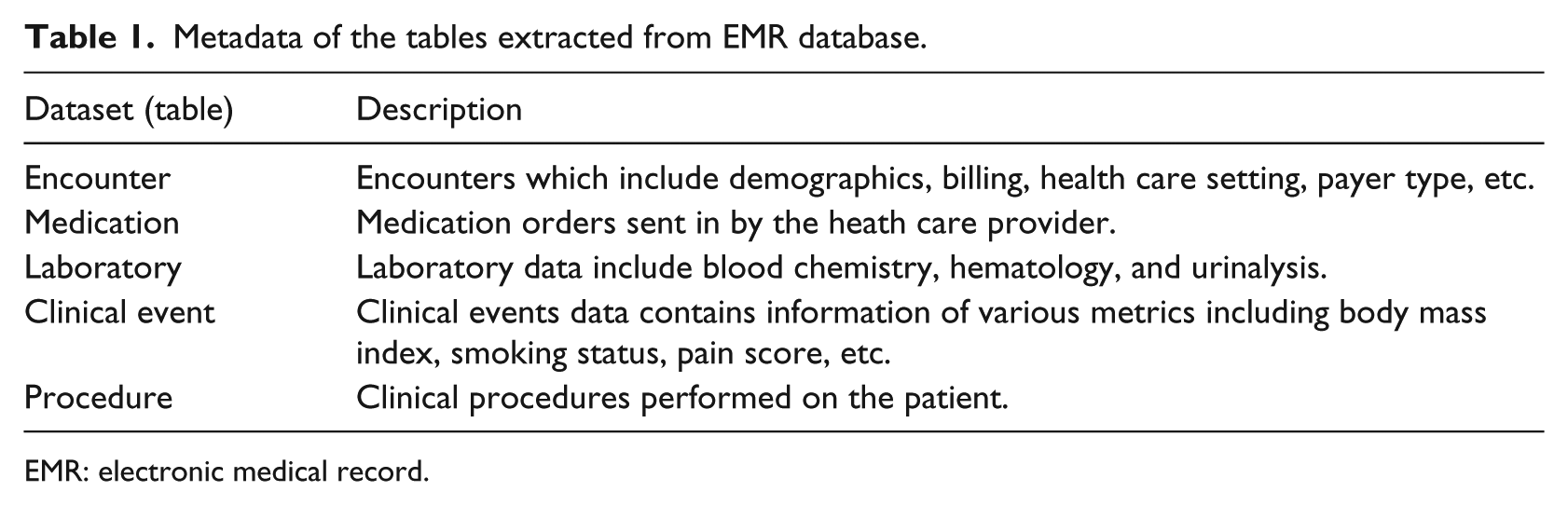
EMR: electronic medical record.

A high-level process flow of the research methodology is shown in Figure 1. Although, the process flow diagram does not give the details of each step, it gives a high-level view of the sequence of the steps performed in the current data mining research study using EMR data. Detailed steps of data balancing and data standardization are explained in the later part of the methods section.

Figure 1.

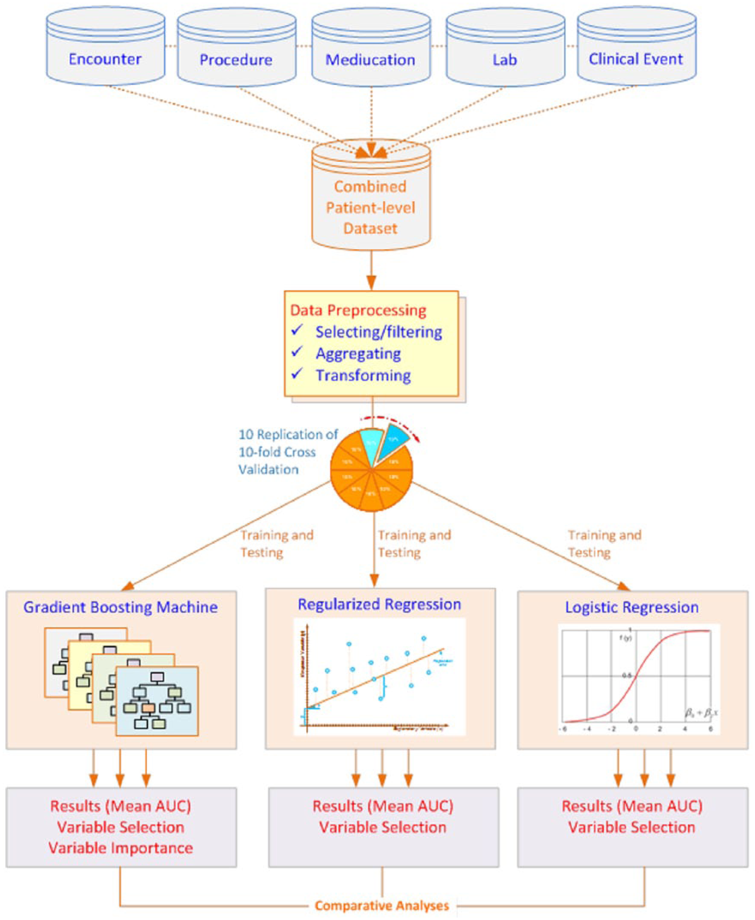
Process flow diagram of the high-level steps involved in the data mining research.

Data cleansing and data preprocessing of EMR data have been a laborious and time-demanding effort. We first extracted patients diagnosed with Crohn’s disease using the International Classification of Diseases, Ninth Revision (ICD 9) code of 555.x. There were a total of 30,150 unique patients in the Cerner health facts database who were diagnosed with Crohn’s disease. The encounter dataset is then merged with the procedure information dataset to create one patient-level dataset. We then filtered to count the number of unique patients that have more than one lab encounter in the database, and we were left with 3335 unique patients, which is approximately 11 percent of the patients that were diagnosed with Crohn’s disease. The first lab encounter is used as the baseline information, and the CRP value from the second lab encounter is used in the computation of the response variable. The next step was to preprocess the lab data to ensure the dataset is analysis-ready. Data preparation is a very time-consuming step, especially with the large amount of real-world EMR data. This preprocessing step takes more than half of the total time, and often times, it may take up to 80 percent of the time spent in a data mining initiative. ³⁰

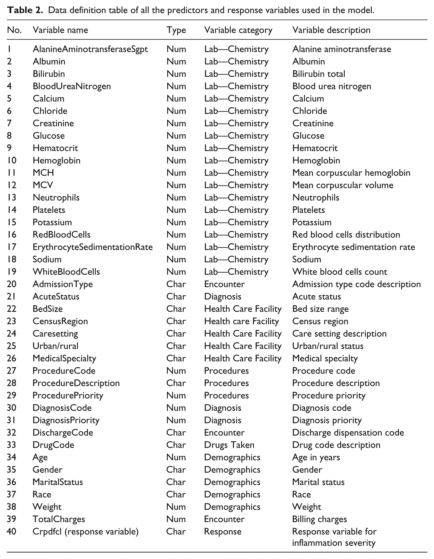
The next step in the preprocessing of the lab data was to standardize the lab test names to one single naming convention. One of the biggest challenges with the EMR data is the missing data. Lab tests ordered by the health care provider vary from patient to patient and are collected at different schedule unlike a clinical trial where data is collected at scheduled intervals. ¹⁴ Due to this limitation, when lab data are transposed to create one record per patient for a lab assessment day, we were left with 189 unique patients that had majority of the variables non-missing. Upon further combining the lab data, encounter data, procedure information, medications, and clinical events, we were left with 82 unique patients to analyze. It is worth noting that the Cerner EMR database has approximately 47 million unique patients in total; however, after filtering for the patients diagnosed with Crohn’s disease and for necessary data used in the prediction of inflammation (CRP) severity, we were left with 82 unique patients. This data size warranted us to use multiple machine learning techniques such as the repeated 10-fold cross-validation, model comparison methods to ensure the predictive models are robust, and the results from the models are repeatable and stable. We believe that the predictive models are more valuable when the predictor list does not include a predictor that is directly linked to the response variable. ³¹ In this study, we dropped the predictor CRP at baseline since our response variable is the CRP doubled from baseline to the next time point. Table 2 shows the complete list of predictors used in the model building along with the response variable.

Table 2.

Data definition table of all the predictors and response variables used in the model.

No.	Variable name	Type	Variable category	Variable description
1	AlanineAminotransferaseSgpt	Num	Lab—Chemistry	Alanine aminotransferase
2	Albumin	Num	Lab—Chemistry	Albumin
3	Bilirubin	Num	Lab—Chemistry	Bilirubin total
4	BloodUreaNitrogen	Num	Lab—Chemistry	Blood urea nitrogen
5	Calcium	Num	Lab—Chemistry	Calcium
6	Chloride	Num	Lab—Chemistry	Chloride
7	Creatinine	Num	Lab—Chemistry	Creatinine
8	Glucose	Num	Lab—Chemistry	Glucose
9	Hematocrit	Num	Lab—Chemistry	Hematocrit
10	Hemoglobin	Num	Lab—Chemistry	Hemoglobin
11	MCH	Num	Lab—Chemistry	Mean corpuscular hemoglobin
12	MCV	Num	Lab—Chemistry	Mean corpuscular volume
13	Neutrophils	Num	Lab—Chemistry	Neutrophils
14	Platelets	Num	Lab—Chemistry	Platelets
15	Potassium	Num	Lab—Chemistry	Potassium
16	RedBloodCells	Num	Lab—Chemistry	Red blood cells distribution
17	ErythrocyteSedimentationRate	Num	Lab—Chemistry	Erythrocyte sedimentation rate
18	Sodium	Num	Lab—Chemistry	Sodium
19	WhiteBloodCells	Num	Lab—Chemistry	White blood cells count
20	AdmissionType	Char	Encounter	Admission type code description
21	AcuteStatus	Char	Diagnosis	Acute status
22	BedSize	Char	Health Care Facility	Bed size range
23	CensusRegion	Char	Health care Facility	Census region
24	Caresetting	Char	Health Care Facility	Care setting description
25	Urban/rural	Char	Health Care Facility	Urban/rural status
26	MedicalSpecialty	Char	Health Care Facility	Medical specialty
27	ProcedureCode	Num	Procedures	Procedure code
28	ProcedureDescription	Char	Procedures	Procedure description
29	ProcedurePriority	Num	Procedures	Procedure priority
30	DiagnosisCode	Num	Diagnosis	Diagnosis code
31	DiagnosisPriority	Num	Diagnosis	Diagnosis priority
32	DischargeCode	Char	Encounter	Discharge dispensation code
33	DrugCode	Char	Drugs Taken	Drug code description
34	Age	Num	Demographics	Age in years
35	Gender	Char	Demographics	Gender
36	MaritalStatus	Char	Demographics	Marital status
37	Race	Char	Demographics	Race
38	Weight	Num	Demographics	Weight
39	TotalCharges	Num	Encounter	Billing charges
40	Crpdfcl (response variable)	Char	Response	Response variable for inflammation severity

The response variable, inflammation severity increased by 100 percent or not, is distributed as 80 percent of the patients in “Yes” class and 20 percent in “No” class. It is very common in real-world medical data that the abnormal class is under-represented. ³² Therefore, balancing the data by over-sampling the under-represented class by empirically proven over-sampling technique such as Synthetic Minority Over-sampling Technique (SMOTE) can help ensure a balance in the data and ensure that the minority class also has good classification accuracy. ³³

The response variable is classified as “Yes” or “No.” The Yes class is assigned when there is a 100 percent or more increase in the CRP value from the baseline to the subsequent visit taken as a percentage. The No class is assigned when the change in CRP value from baseline to the subsequent visit is less than 100 percent.

$$\mathrm{Difference}\mathrm{in}\mathrm{CRP}=\frac{\left(\mathrm{CRP}\mathrm{follow-up}-\mathrm{CRP}\mathrm{baseline}\right)}{\mathrm{CRP}\mathrm{baseline}}\times 100$$

If difference in CRP is greater than or equal to 100 percent, response = “Y”; and if the difference in CRP is less than 100 percent, the response = “N.”

Method

This study used multiple software products to extract, cleanse, transform, explore the data, and to build predictive models and to visualize the results. Specifically, SAS 9.4 software has been used in the data processing, data cleaning, and having analysis-ready dataset in preparation of the predictive modeling. JMP 12.0 software from SAS was used in the data exploration step. The predictive modeling step was performed using the open-source software R. This research utilized logistic regression, regularized regression and gradient boosting machines (GBM) algorithms to perform predictive modeling. The most popular “gbm” package from R was used for GBM. “glmnet” package was used for regularized regression and “glm” for the logistic regression model. To test the robustness of the predictions, this study used two linear models and one non-linear model. We developed the first model which was a traditional logistic regression and modeled the function of severity of inflammation doubling with all the predictors that are identified in the data description Table 2.

The second method was the regularized regression, which would place penalty and shrink the coefficients of the less-relevant predictors. The third method was the non-linear GBM method, which was a non-parametric tree-based method. The rationale for selecting regularized regression in addition to logistic regression is that with EMR data, there are a large number of predictors in the predictive model, and regularized regression has a mechanism to place penalty and shrink the coefficients of the less-relevant predictors to zero with the lasso step in the regularized regression. The ridge regression step within the regularized regression places penalty on the less-relevant predictors and shrinks the coefficients closer to zero. Therefore, the regularized regression algorithm is a good choice for pruning variables that are of no predictive value which at the end makes the model more interpretable with less predictors.

Logistic regression

Logistic regression is one of the linear methods that we have used in the predictive modeling exercise. p(X) is the function that is modeled which provides probability output between 0 and 1 for all values of X, where X₁–X_p are the predictors. This is the probability that the patients would have inflammation severity increased 100 percent or not. The coefficients β₀–β_p are estimated using maximum likelihood estimation

$$\mathrm{p}\left(\mathrm{X}\right)=\frac{{\mathrm{e}}^{{\beta }_0+{\beta }_1{\mathrm{X}}_1+\cdots +{\beta }_{\mathrm{p}}{\mathrm{X}}_{\mathrm{p}}}}{{1+\mathrm{e}}^{{\beta }_0+{\beta }_1{\mathrm{X}}_1+\cdots +{\beta }_{\mathrm{p}}{\mathrm{X}}_{\mathrm{p}}}}$$

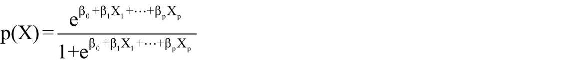
The coefficients are interpreted as for a unit increase in the predictor, the log odds of the patient severity increasing Yes/No will increase by so many units holding all other predictors constant.

Regularized regression

Regularized regression is a combination of the lasso regression and the ridge regression. The regularized method tries to balance the model performance and the complexity of the model. The two methods, ridge regression and lasso regression, are utilized to optimize the specific loss function using all the available data in the learning sample. The maximum likelihood method tends to over fit the data when the number of predictors is large. Therefore, the regularized regression method is proposed to be more robust when large number of predictors are used in the model. This ensures a balance between the bias and variance problem. The lasso method is jointly optimizing the mean squared error (MSE) and the L1 norm of the coefficients. The ridge method is jointly optimizing the MSE and the L2 norm of the coefficients $(\mathrm{Mean}\mathrm{Squared}\mathrm{Error}+\lambda \times \mathrm{Model}\mathrm{Complexity})$ :

• Ridge: sum of squared coefficients;

• Lasso: sum of absolute coefficients;

• λ: regularization parameter.

When λ = 0, the ridge regression is same as the logistic regression. The objective function for regularized logistic regression can be expressed as

$$\frac{1}{\mathrm{N}}{\displaystyle \sum }_{\mathrm{i}=1}^{\mathrm{N}}{\mathrm{y}}_{\mathrm{i}}*\left({\beta }_0+{\mathrm{X}}_{\mathrm{i}}^{\mathrm{T}}\beta \right)-\log \left(1+{\mathrm{e}}^{({\beta }_0+{\mathrm{X}}_{\mathrm{i}}^{\mathrm{T}}\beta )}\right)+\lambda \left[\frac{\left(1-\alpha \right){\left||\beta |\right|}_2^2}{2}+\alpha {\left||\beta |\right|}_1\right]$$

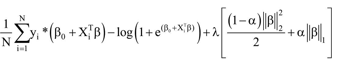
The minimum of $\beta$ is selected from the above equation over a range of values of λ from 0 to 1. Optimal value of λ is selected from the cross-validation error by selecting the minimum mean-cross-validation error or the error that is 1 standard error away from the minimum. The ridge penalty, which is the L2 norm, shrinks the coefficients of the correlated predictors toward each other while the lasso penalty, which is the L1 penalty, tends to select one of the predictor and drop the other correlated predictor. The elastic net penalty is controlled by a tuning parameter called α; where $\alpha =(\lambda 2+\lambda 1)/(\lambda 1)$ for $\mathrm{J}(\beta )=\alpha {|\beta |}^2+(1-\alpha )||\beta |$ .

GBM

GBM is a non-parametric tree-based ensemble model that has been developed to solve classification- and regression-type problems. The trees are built using recursive binary partition techniques that split data into regions taken from the Classification and Regression Trees (CART). ³⁴ A single weak tree is built with minimal number of nodes, and the prediction is made. Sequentially, grow a second tree to predict the residual from the first tree and continue the tree building until the preassigned number of trees are built with the same node size for all the trees using the loss function. The logistic loss function is the amount of penalty incurred when the model predicts h(x) on the observed outcome Y. Function h(x) is the log odds of

$$\mathrm{Y}=\frac{1}{\mathrm{N}}{\displaystyle \sum _{\mathrm{i}=1}^{\mathrm{N}}\log \left(1+{\mathrm{e}}^{-{\mathrm{y}}_{\mathrm{i}}\cdot 2\cdot {\mathrm{h}(\mathrm{x}}_{\mathrm{i}})}\right)}$$

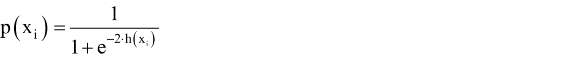
This loss function is referred to as the Bernoulli loss function. The probability of x_i ∈ class Y = 1 is computed as

$$\mathrm{p}\left({\mathrm{x}}_{\mathrm{i}}\right)=\frac{1}{1+{\mathrm{e}}^{-2\cdot \mathrm{h}\left({\mathrm{x}}_{\mathrm{i}}\right)}}$$

This research has used 1000 trees with a node size of 10 run on a 10 × 10-fold to make the predictions. A higher interaction depth is allowed for more interaction between the predictors.

Cross-validation—10 × 10-fold

Cross-validation method is one of the most frequently used technique in the predictive modeling problem. K-fold cross-validation ³⁵ is used to split the data into K equal parts, where the model is built on the training set, and the model performance is tested using the test set. Breiman et al. ³⁴ and Kohavi ³⁵ and many recent studies have shown that 10-fold cross-validation method is optimal to reduce bias and overfitting of the data. However, replicability of the results is not achieved to a greater extent. Therefore, this research has used the 10 times repeated 10-fold cross-validation method. This would result in creating 100 models and generating 100 predictions for each patient. Empirical study has shown that 10 times repeated 10-fold cross-validation to produce more replicable results and low type 1 error compared to a 10-fold cross-validation or a hold-out sample method. ³⁶

In this research, the mean area under the curve (AUC) from each run out of the 10 repeated runs is computed. The mean AUC for the first run is the average of the AUCs across all folds from the first run out of the 10 repetitions. Likewise, mean AUC₂, AUC₃, …, AUC₁₀ are generated for each model.

Results

Prediction results are generated using the test set applying the repeated 10 times run on 10-fold cross-validation set. Performance of each model is assessed by the metric, AUC, which has been the preferred performance metric over the prediction accuracy since the receiver operating characteristics (ROC) curve, which generates the AUC, compares the classifier performance across the entire range of class distributions and error costs; hence, it is widely accepted as the performance measure for machine learning applications.^37,38 The mean AUC from the 10 times repeated 10-fold cross-validation is generated for the three models: logistic regression, regularized regression, and the GBM.

Mean AUC metric in Figure 2 and Table 3 indicates that GBM model is the best performing model with a mean AUC of 92.82 percent and a median AUC of 93.43 percent from each repeated run across the 10 folds. The second best performing model is the regularized regression with a mean AUC of 82.70 percent and a median AUC of 82.74 percent. The worst performing model among the three models is the logistic regression with a mean AUC of 81.12 percent and a median AUC of 81.24 percent. The box plot shows the median AUC as a dark bar, with the box width showing the center quartiles of the AUCs and the whiskers showing the outer quartiles of the AUCs. It is worth noting that GBM, which is the tree-based method, performs significantly better than the traditional linear methods: logistic regression and the regularized regression methods. The performance of regularized regression and the logistic regression is almost similar except that the regularized regression has slightly higher prediction accuracy. This could be a resultant of the penalty of the lambda applied on the non-relevant predictors.

Figure 2.

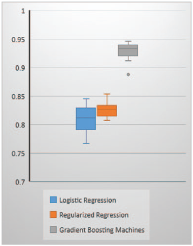
Mean AUC across 10 folds within each repeated run.

Table 3.

AUC for each repeated run across three models.

Repeated run	Logistic regression	Regularized regression	Gradient boosting machines (GBM)
1	0.7929	0.8267	0.9393
2	0.7878	0.8078	0.9262
3	0.8080	0.8145	0.9369
4	0.8461	0.8487	0.9124
5	0.8243	0.8281	0.9414
6	0.7681	0.8543	0.8878
7	0.8167	0.8154	0.9356
8	0.8174	0.8176	0.9330
9	0.8452	0.8281	0.9467
10	0.8050	0.8294	0.9230
Mean AUC	0.8131	0.8271	0.9282
Median AUC	0.8167	0.8274	0.9343

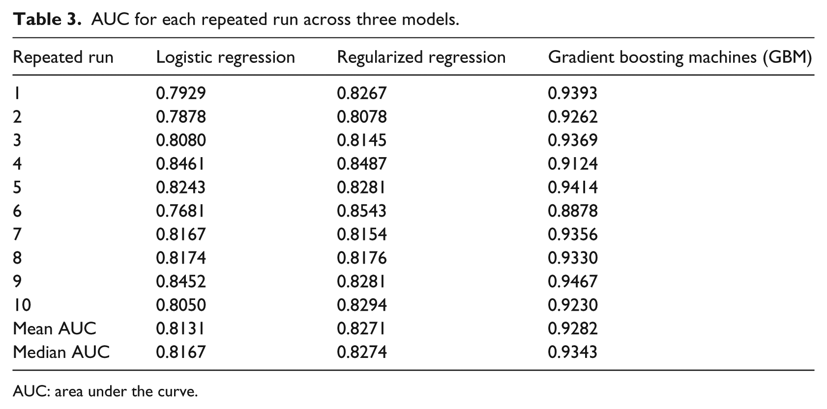
AUC: area under the curve.

Upon generation of the AUCs for 100 models, we have performed a post hoc analysis of variance (ANOVA) test and applied the Tukey’s honestly significant difference (HSD) test for multiple comparison tests to determine which classifier method’s performance differs from the other based on the AUC. A number of statistical techniques have been tested to show the differences in the classifiers from each machine learning method. Dietterich ³⁹ has examined five different tests to understand the difference in classifier performance such as McNemar test, a test for difference in two proportions, a paired difference t-test, a paired difference t-test on 10-fold cross-validation results, and a 5 × 2-fold cross-validation results as a paired difference. The conclusion from all these tests was that no single method works best in all situations. McNemar test works best when the algorithm is executed only once, whereas the 5 × 2 cross-validation works best when the algorithms are executed multiple times. Research by Demšar ⁴⁰ shows that non-parametric tests such as Wilcoxon and Freidman tests perform better than the parametric tests in classifier performance comparison tests. However, there is no gold standard for making such comparisons since each test has different assumptions and so can yield different results from each method.

Tukey’s HSD post hoc test is similar to the t-test except that the critical values tabulated are higher for Tukey’s test to ensure that there is a maximum of 5 percent chance that one of the pairwise comparisons is erroneously identified as statistically significant

$$\mathrm{Tuke}{\mathrm{y}}^{\prime }\mathrm{s}\mathrm{HSD}=\mathrm{q}\sqrt{\frac{{\mathrm{MS}}_{\mathrm{within}}}{n}}$$

The value of q is the table value and the MS_within is the mean square difference within a group and n is the number of values within each group.

The test results show that the mean AUC for regularized regression and the logistic regression are not significantly different from each other. However, the AUC from regularized regression and logistic regression are significantly different from the GBM model as seen in Table 4.

Table 4.

ANOVA with multiple comparisons using Tukey’s test.

Mean values with the same letter are not significantly different
Tukey grouping	Mean AUC	No. of observations	Model type
A	0.928	100	GBM
B	0.827	100	Regularized regression
B	0.812	100	Logistic regression

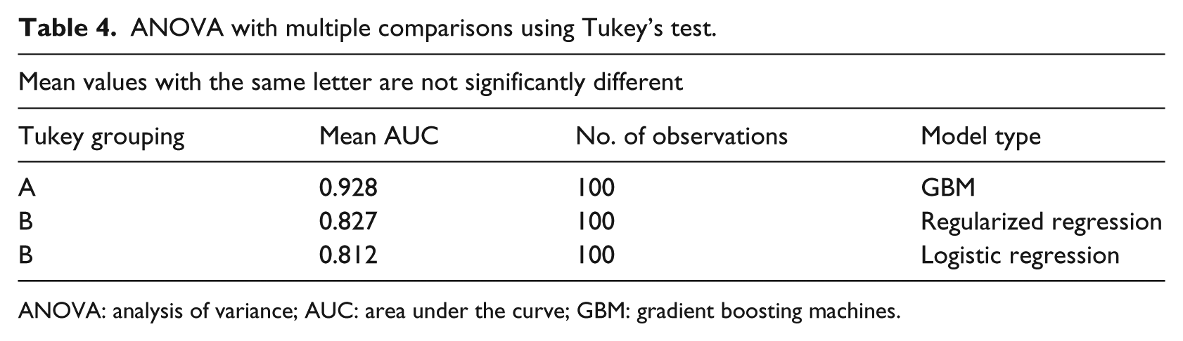
ANOVA: analysis of variance; AUC: area under the curve; GBM: gradient boosting machines.

Feature or variable selection is an important component in detecting the discriminating features or variables out of a large number of variables. Variable importance is a relative measure that identifies the important predictors for predicting the response. Variable importance in tree-based methods is measured using the Gini index, cross entropy, or the relative decrease in accuracy. Relative importance in GBM is computed using Gini index. Gini index is a total variance or the node impurity across the K classes, which is two classes in our study

$$\mathrm{Gini\; index},\mathrm{G}={\displaystyle \sum _{\mathrm{k}=1}^{\mathrm{K}}{\widehat{P}}_{\mathrm{mk}}(1-{\widehat{P}}_{\mathrm{mk}})}$$

Relative importance is computed by adding up the total amount of decrease in Gini by the splits over a given predictor, averaged across all the trees specified in the GBM tuning parameter, which is 1000 trees in our research. This average decrease in Gini is normalized to a 0-to-100 scale, where higher number indicates stronger predictor. Our model results in Figure 3 show that it is not one single predictor driving the predictions. It is a combination of predictors driving the predictions. Crohn’s disease location at diagnosis such as small intestine, large intestine, lab parameters at baseline such as white blood cell (WBC) count, mean corpuscular hemoglobin (MCH), mean corpuscular volume (MCV), sodium, red blood cell (RBC) distribution, platelet count, creatinine, hematocrit, and hemoglobin are the strongest predictors. Demographic predictors such as age is one of the strongest predictors of the inflammation severity doubling. There are other health care settings and encounter-related variables such as hospital bed size, diagnosis priority, diagnosis and region, whether south or not, predicting whether inflammation severity doubled or not also having some predictive ability. Majority of the Crohn’s disease researchers identified location of the disease, age at diagnosis, smoking status, biologic markers, and TNF levels to predict the response to treatment, which are some of the identifiers that also predicted the inflammation severity. ²¹ Logistic regression and regularized regression cannot produce a similar relative variable importance plot. However, the odds ratio and standardized coefficients generated are used in identifying the stronger predictors that can predict the inflammation severity.

Figure 3.

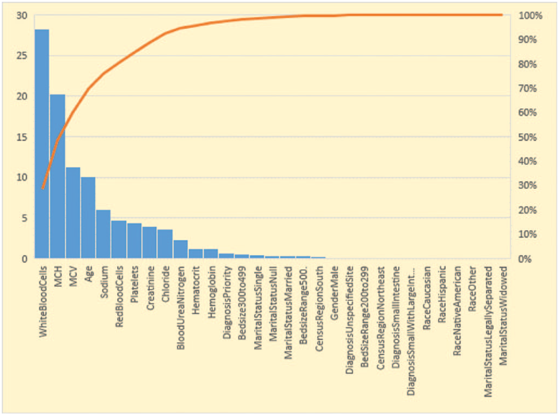
Relative variable importance for GBM model.

In addition to the variable importance, this study also looked at the stability of the predictors that were identified as important predictors. The 10 times repeated 10-fold cross-validation would result in 100 models. This research quantitatively assessed the number of occurrences of each predictor out of the 100 runs. A value of 100 from the figure shows that the specific predictor was selected in all the 100 models. It is worth noting that all the predictors in the variable importance figure appear in higher than 90 percent of the models as shown in Figure 4. There are a few statistical tests to check the stability of the predictors such as Jaccard index and Spearman coefficient. Jaccard index looks at the overlap of the predictors from each run while Spearman coefficient looks at the sequence or the order of the predictors in the variable importance. In this research, we have primarily focused on comparing the variable importance list with the variable importance stability. Prior research has shown that instability in the variable importance is caused not only by data perturbations or parameter variations but also from intrinsic randomness of the variable importance measures. ¹⁵

Figure 4.

Variable selection frequency for GBM model.

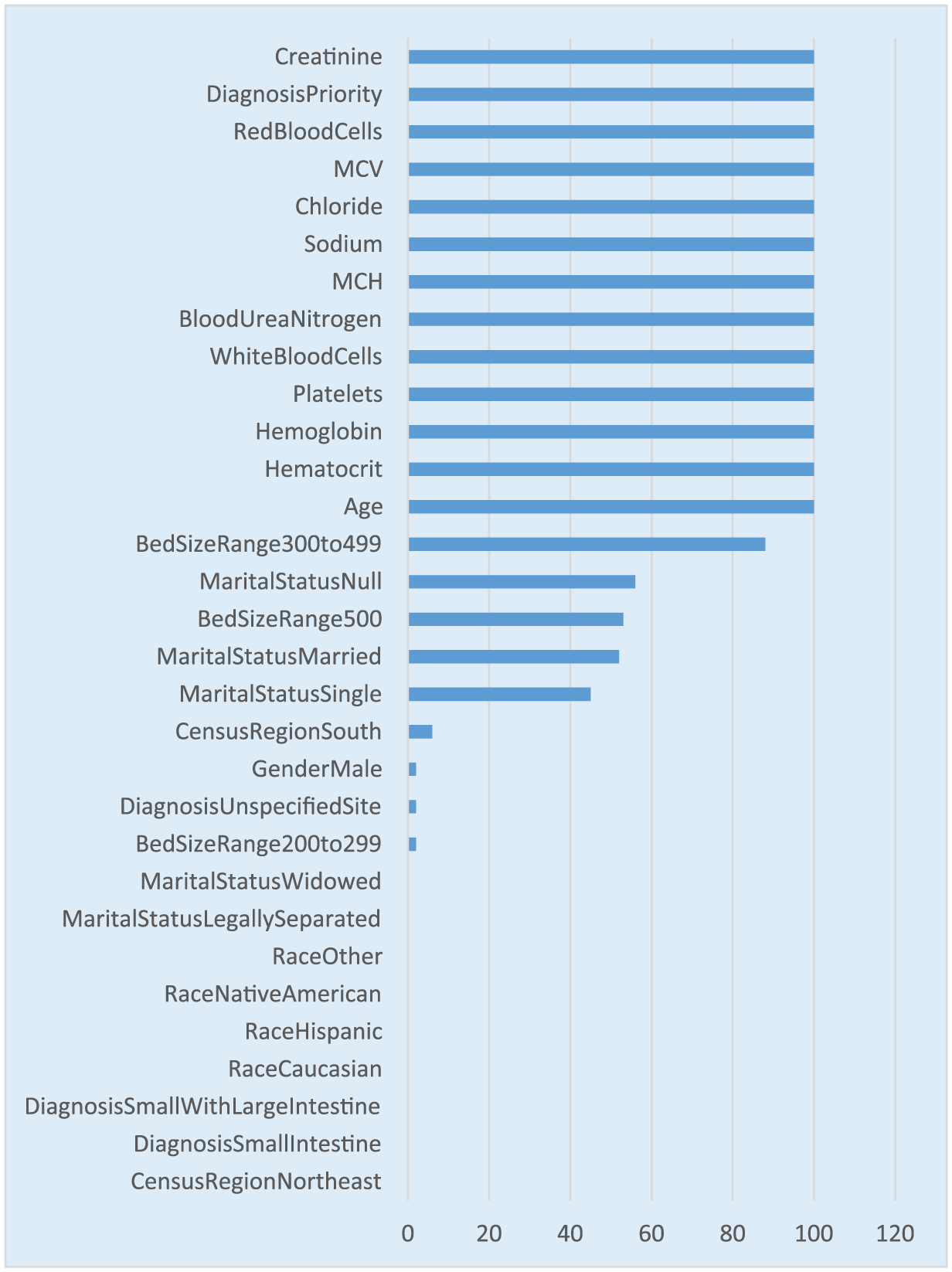
Variable or feature selection metric in regularized and logistic regression is extracted by analyzing the standardized coefficients and the odds ratio along with the p-value for each predictor. However, the stability of the predictor is still tested by comparing the number of times each predictor occurs in the model with an estimate greater than zero and a p-value < 0.05 out of the 100 models. It is worth noting that the regularized regression has less number of predictors occurring in the 100 models compared to the logistic regression due to the fact that regularized regression shrinks the less-relevant coefficients to zero. This process reduces the number of times a predictor occurs in the model (see Figure 5).

Figure 5.

Variable selection frequency for regularized regression.

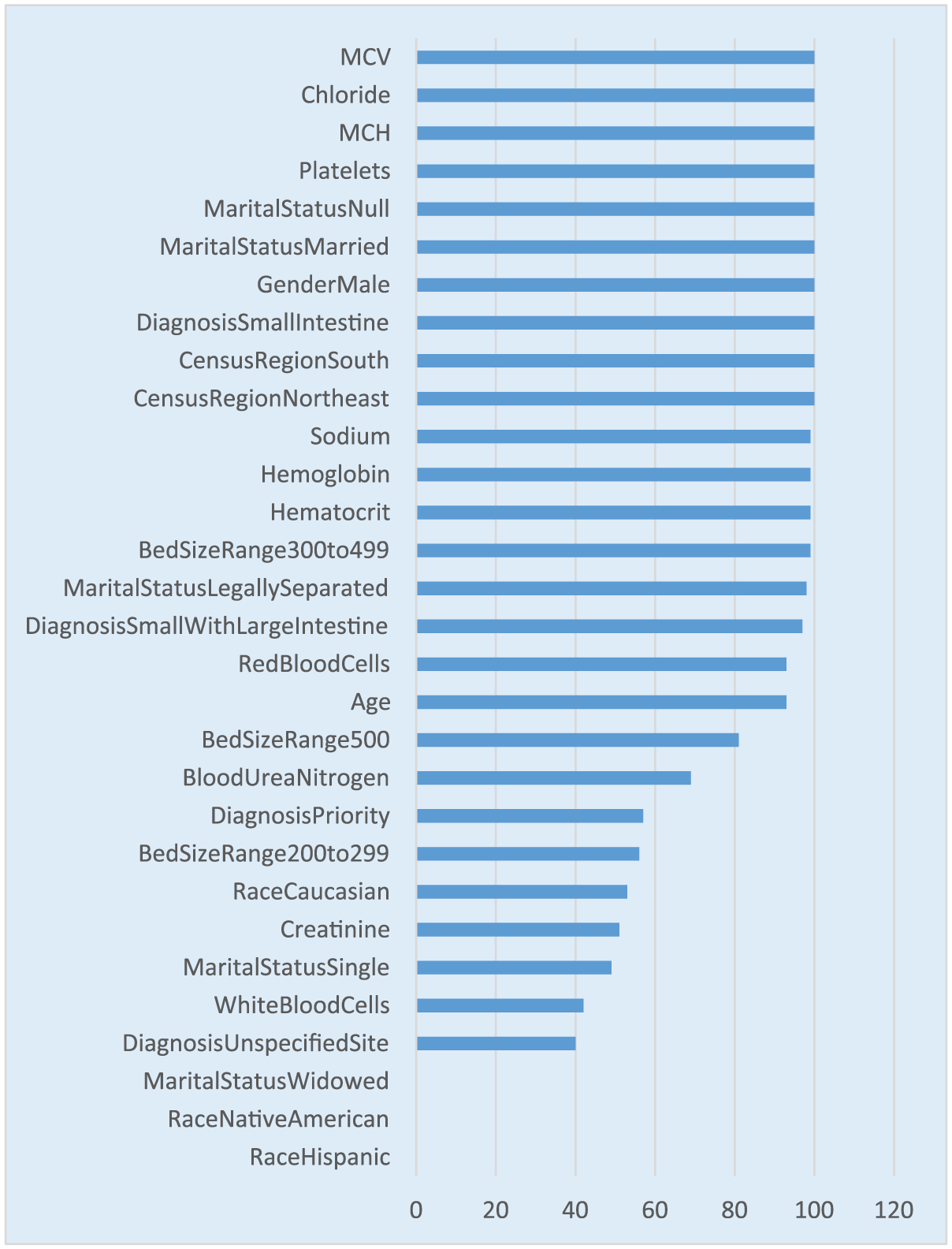
It is worth noting that the predictors or features occurring 100 percent of the times in the regularized regression in Figure 5 also occur 100 percent in the logistic regression model as shown in Figure 6. However, regularized regression has a smaller list of predictors occurring in all 100 models with a coefficient not equal to zero and a p-value < 0.05 (see Figure 5).

Figure 6.

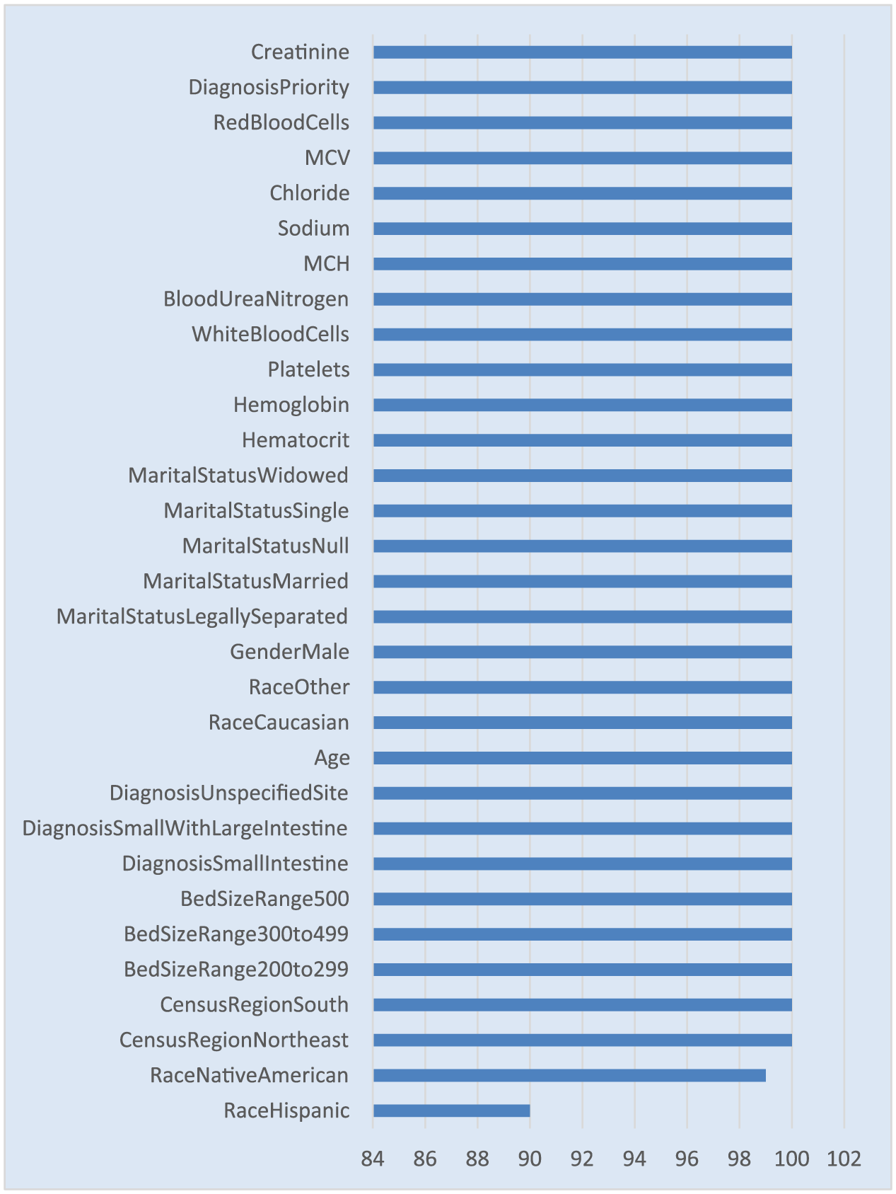
Variable selection frequency for logistic regression.

Summary, conclusion, and future directions

This research focused on building predictive models using EMR data. The exponential growth of availability of EMRs has facilitated researchers to develop analytic models to predict an event or a disease condition for a patient, which enables better patient care. ⁴¹ The model performances are very encouraging and promising. It is worth noting that the data mining algorithm, GBM, performed significantly better compared to the traditional linear models, both logistic regression and regularized regression. The predictors identified from all the models show that baseline laboratory parameters such as WBC, MCV, hematocrit, RBC, are some of the strongest predictors in addition to demographic variables such as age, gender, diagnosis priority, and other health care setting variables such as geographic location. It is evident that one single predictor cannot explain the prediction, but a combination of predictors is required to predict the inflammation severity. The limitation of this study is the lack of patient-reported outcome (PRO) data in the EMR data that could have been used as a composite variable in addition to the CRP. PRO data consist of the questionnaire data related to pain score, number of stools, etc., which may have further boosted the prediction accuracy when taken as a composite with CRP.

With this study, we were able to show that disease management can be done real-time using decision support tools that would predict the future inflammation state, which would then allow for medical intervention prospectively. The health care providers are able to improve patient outcomes by intervening early on and making necessary therapeutic adjustments that would work for the specific patient. This approach begins to evolve toward personalized or precision medicine. The response variable, CRP, difference that is being predicted is collected at a low cost and is very non-invasive in nature compared to surgical procedures. In addition, we were able to demonstrate that although the EMR data are very large in size, we might only be left with a small portion of subjects after filtering for all the conditions and after taking into consideration the missing and incomplete data.

The future research in this area could be to look at the EMR data and identify the comorbid conditions for patients with Crohn’s disease since CRP is very predominantly used as a predictor of other life-threatening diseases. The additional future area of research is to utilize the longitudinal time-varying patient data in Crohn’s disease and build models that are able of capturing the temporal aspects of the patient test results and finally build individualized probability curves that explain the disease state.