Sage Journals: Discover world-class research

Abstract

Introduction:

Obstructive sleep apnea syndrome has become an important public health concern. Polysomnography is traditionally considered an established and effective diagnostic tool providing information on the severity of obstructive sleep apnea syndrome and the degree of sleep fragmentation. However, the numerous steps in the polysomnography test to diagnose obstructive sleep apnea syndrome are costly and time consuming. This study aimed to test the efficacy and clinical applicability of different machine learning methods based on demographic information and questionnaire data to predict obstructive sleep apnea syndrome severity.

Materials and methods:

We collected data about demographic characteristics, spirometry values, gas exchange (PaO₂, PaCO₂) and symptoms (Epworth Sleepiness Scale, snoring, etc.) of 313 patients with previous diagnosis of obstructive sleep apnea syndrome. After principal component analysis, we selected 19 variables which were used for further preprocessing and to eventually train seven types of classification models and five types of regression models to evaluate the prediction ability of obstructive sleep apnea syndrome severity, represented either by class or by apnea–hypopnea index. All models are trained with an increasing number of features and the results are validated through stratified 10-fold cross validation.

Results:

Comparative results show the superiority of support vector machine and random forest models for classification, while support vector machine and linear regression are better suited to predict apnea–hypopnea index. Also, a limited number of features are enough to achieve the maximum predictive accuracy. The best average classification accuracy on test sets is 44.7 percent, with the same average sensitivity (recall). In only 5.7 percent of cases, a severe obstructive sleep apnea syndrome (class 4) is misclassified as mild (class 2). Regression results show a minimum achieved root mean squared error of 22.17.

Conclusion:

The problem of predicting apnea–hypopnea index or severity classes for obstructive sleep apnea syndrome is very difficult when using only data collected prior to polysomnography test. The results achieved with the available data suggest the use of machine learning methods as tools for providing patients with a priority level for polysomnography test, but they still cannot be used for automated diagnosis.

Keywords

machine learning obstructive sleep apnea syndrome

Introduction

Obstructive sleep apnea syndrome (OSAS) is a very common disorder with incidence estimated at 5–14 percent among adults aged 30–70 years.¹ Recent studies have demonstrated that the prevalence of events of obstructive sleep apnea not associated with sleepiness could affect about 50 percent of men and 23 percent of women.² The clinical importance of OSAS is related to increased risk of cardiovascular diseases as well as higher morbidity and mortality.³

The gold standard for diagnosis of OSAS is the polysomnography (PSG) test⁴ through which it is possible to have information on the severity of OSAS and the degree of sleep fragmentation. However, PSG requires overnight evaluation in a sleep laboratory, dedicated systems and attending personnel. Other methods are used to simplify the diagnosis of OSAS, such as cardiorespiratory monitoring or O₂ pulse oximeter overnight. However, these alternative methods require patients to bear diagnostic instruments for at least one night, with consequent nuisance; also, low availability of such instruments could lead to long waiting lists. As the number of subjects with suspected OSAS increases, the need of simple and effective diagnostic methods becomes more and more compelling.

In the past few years, some predictive models have been developed, which are mainly based on self-reported symptoms, demographics, anthropometric variables and comorbidities.^5–7 The choice of screening method may change according to the type of population (general or sleep center referrals) and the screening objective, the latter being either to support the decision of selecting the most appropriate sleep testing or to prioritize patients according to the severity of their case. A good screening method should incorporate an estimation of severity of disease according to some descriptive parameters such as apnea/hypopnea index (AHI), oxygen desaturation index (ODI) or time of hypoxia (T90), as well as to correlations with observed symptoms such as sleepiness, fatigue, cardiovascular outcomes and impact of comorbidities. No screening tool has proven to be the best one so far and new methods need to be tested.

Recently, new methods of data analysis such as artificial neural networks have been applied in Medicine to analyze large amounts of clinical data to better understand the pathogenetic mechanisms or to improve the ability to diagnose some pathologies. These methods, falling in the field of machine learning, have powerful problem-solving capabilities and have several advantages in detecting the possible interactions among many variables, and hence they may be useful in clinical prediction.⁸ In the last years, several studies have been carried out also on OSAS to evaluate the ability of machine learning methods to predict the disease or to estimate its severity.^9,10 However, even if the results are encouraging, few data are available for the application of these methods in routine clinical setting. The lack of large numbers of patients, together with the high number of features that are involved to describe the clinical status of each patient, may pose severe limitations to the effectiveness of machine learning models.

In order to understand the real clinical applicability of these methods in managing the OSAS, in this study we test the ability of different machine learning methods to predict the severity of obstructive sleep apnea in a relatively large cohort of patients and define the power, advantages and also the limitations of each method.

Materials and methods

We collected the data of consecutive patients from the sleep centers of the Universities of Foggia and Milan, in which all subjects underwent a general information questionnaire about clinical parameters (age, body mass index (BMI), neck circumference, Mallampati scale, smoking history), sleep propensity (according to Epworth Sleepiness Scale (ESS)), other questions about symptoms and the presence of comorbidities (cardiovascular diseases, diabetes, hypertension, etc.). Moreover, data of blood gas analysis and spirometry were also collected. Finally, all subjects underwent a cardiorespiratory monitoring to assess the presence and severity of obstructive sleep apnea according to AHI, ODI and T90. Patients with central sleep apnea and neuromuscular diseases were excluded.

The software tools Knime (https://www.knime.com/), Mathematica (http://www.wolfram.com/mathematica/) and Orange (https://orange.biolab.si/) have been used to design the machine learning predictive models used in this work.

The study was approved by the Ethic Committee of the Ospedali Riuniti di Foggia. Written informed consent to collect and analyze data was obtained from all participants and all data were anonymized prior to analysis.

Dataset

The processed dataset is made of 313 samples (patients with OSAS diagnosed according to American Association of Sleep Medicine (AASM) guidelines) described by 32 numerical or nominal features (Table 1), related to a target variable Severity corresponding to four classes of disease severity as defined by American Academy of Sleep Medicine Task Force¹¹ (Table 2). Among all features, only PaO₂, FVC% (forced vital capacity) and FEV₁% (forced expiratory volume in the first second) passed the Shapiro–Wilk test of normality.

Table 1.

Descriptive statistics of the available dataset.

Feature	Mean	Standard deviation	Range
Age (years)	60.42	12.42	20–85
Sex	Male: 76%; female: 24%
BMI (kg/m²)	36.49	8.86	16–65.92
ESS	10.69	5.41	0–24
Smoke	Yes: 68%; no: 32%
Mallampati score	2.38	1.06	1–4
Snore	3.47	0.84	1–4
Tiredness in the morning	3.38	1.51	1–5
Choking	0.88	0.81	0–2
Sweating frequency	0.42	0.71	0–3
Reported apneas	3.63	1.47	0–5
Reported headaches	0.47	0.67	0–2
Reported concentration difficulties	0.49	0.67	0–2
Reported memory difficulties	0.53	0.67	0–2
Falling asleep at the wheel	1.21	0.98	0–5
Chronic obstructive pulmonary disease	Yes: 17%; no: 83%
Asthma	Yes: 5%; no: 95%
Hypertension	Yes: 72%; no: 28%
Heart disease	Yes: 39%; no: 61%
Diabetes	Yes: 34%; no: 66%
Dyslipidemia	Yes: 30%; no: 70%
Dysthyroidism	Yes: 12%; no: 88%
Carotid atheroma	Yes: 6%; no: 94%
Depression	Yes: 8%; no: 92%
Other neurological disorders	Yes: 7%; no: 93%
Neoplasms	Yes: 9%; no: 91%
Gastroesophageal reflux disease	Yes: 16%; no: 84%
PaO₂ (mmHg)	77.45	12.42	46–116
PaCO₂ (mmHg)	41.67	5.55	28–70
FVC%	97.07	20.73	31–160
FEV₁%	91.88	21.78	40–183
FEV₁/FVC	76.15	10.12	35–116

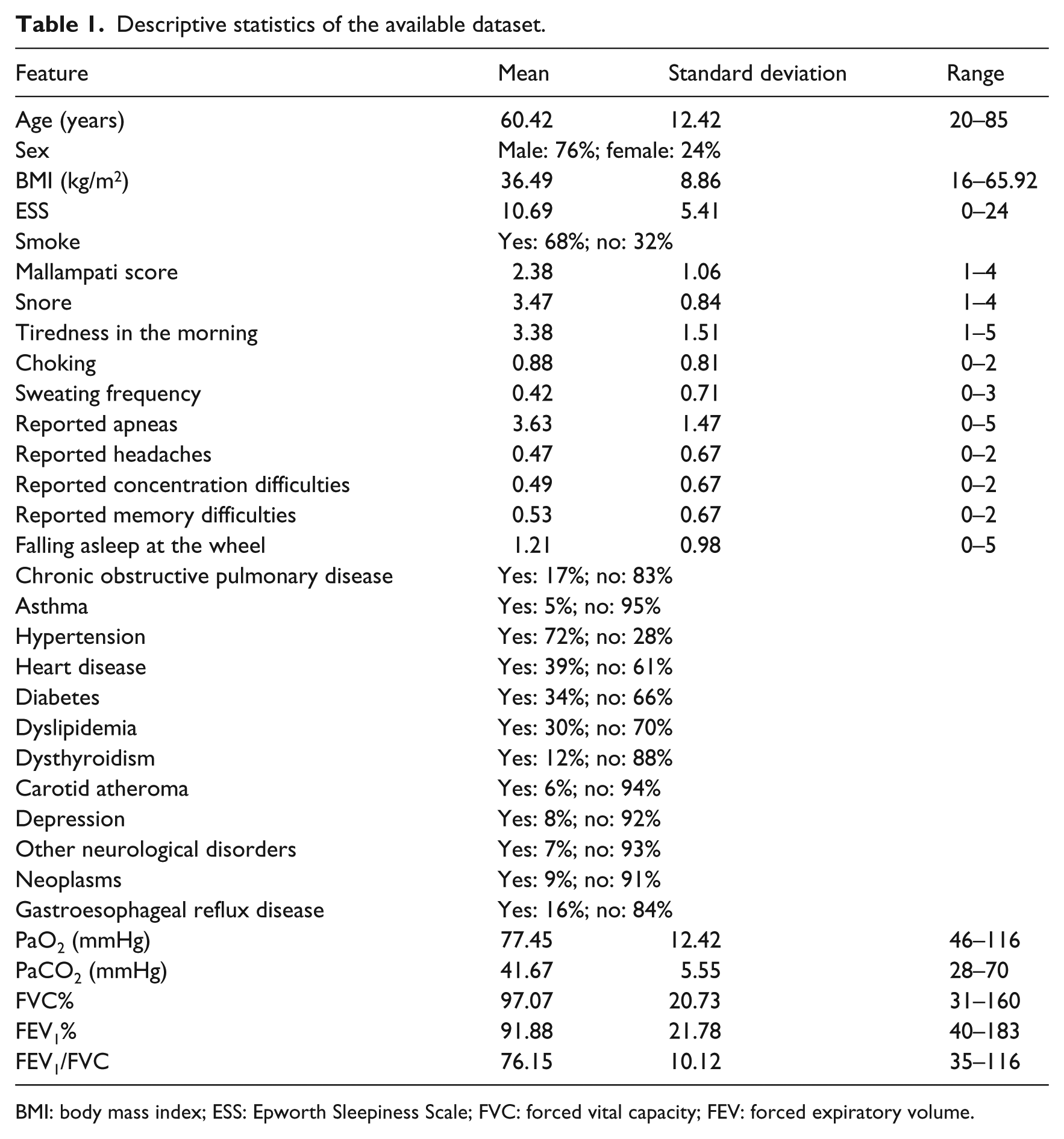
BMI: body mass index; ESS: Epworth Sleepiness Scale; FVC: forced vital capacity; FEV: forced expiratory volume.

Table 2.

AASM severity classes for OSAS and their distribution in the available dataset.

Severity class	AHI interval	Subjects	Ratio (%)
1 (normal)	5–15	25	7.98
2 (mild)	16–30	65	20.77
3 (moderate)	31–60	117	37.38
4 (severe)	61+	106	33.87

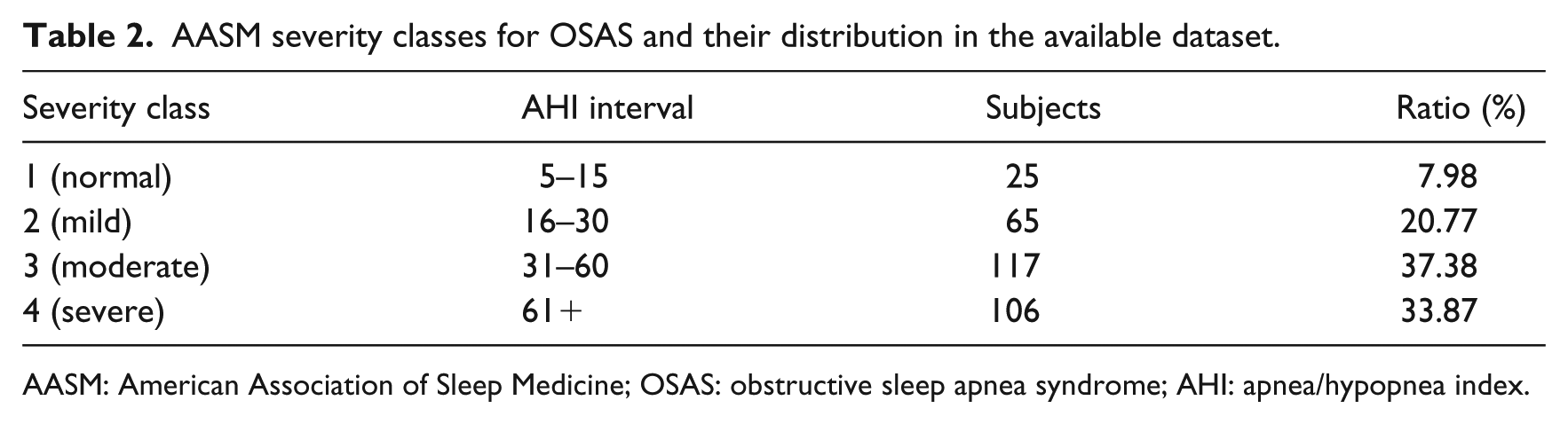
AASM: American Association of Sleep Medicine; OSAS: obstructive sleep apnea syndrome; AHI: apnea/hypopnea index.

Preprocessing

Preliminary feature selection

The primary goal of preprocessing is the selection of a suitable subset of features that will be used to design the predictive models. To this end, since the original number of features is very high when compared to the number of samples, we proceeded with a preliminary selection of features.

The selection was carried out through the principal component analysis (PCA) applied to the original dataset. Starting from the dataset of the clinical situation of the patients, the correlation matrix was calculated (using Spearman rank correlation coefficients because of the non-normality of data distribution) among the initial 32 features. Then, Bartlett’s test of sphericity and Kaiser–Meyer–Olkin (KMO) sampling adequacy were applied to the correlation matrix, both leading to a significant distribution of the dataset variability (p < 0.05), which justified the subsequent PCA by means of which seven main components, corresponding to the seven eigenvalues ⩾ 1, were extracted. The final selection of 19 features was then carried out by examining the contribution of the 32 initial features to the sevn major components, ranking them through their communality index and selecting only those having an index ⩾ 0.50 (Table 3). The selected features have been validated by D.L., who is an expert in sleep medicine.

Table 3.

Selected features after preliminary preprocessing with PCA, ranked by their communality index.

Feature	Communality index
FEV₁%	0.86
Heart disease	0.81
Diabetes	0.80
Sex	0.79
FVC%	0.78
BMI	0.73
Age	0.68
ESS	0.68
Smoke	0.62
Falling asleep at the wheel	0.62
Mallampati score	0.62
Choking	0.62
PaCO₂	0.60
Tiredness in the morning	0.58
Hypertension	0.58
PaO₂	0.55
Reported apneas	0.55
Snore	0.54
FEV₁/FVC	0.54

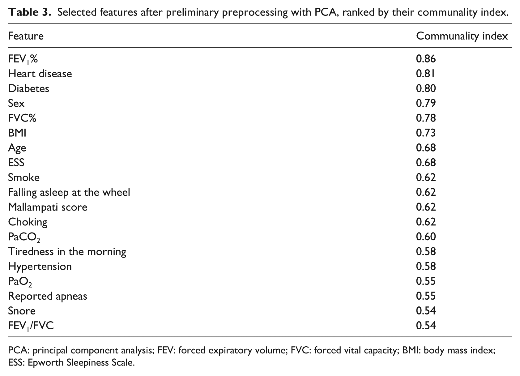
PCA: principal component analysis; FEV: forced expiratory volume; FVC: forced vital capacity; BMI: body mass index; ESS: Epworth Sleepiness Scale.

Feature ranking and selection

The feature set resulting from preliminary feature selection has been processed in order to further reduce the number of features that are used for generating the predictive models. In this way, we attenuate the risk of overfitting resulting from the use of too many features on a dataset characterized by few samples (this risk is further exacerbated when non-linear predictive models are used).¹²

Among several feature selection methods, we focus on those based on feature ranking, which reveal the relative importance of each feature in determining the value of the target variable.¹³ Given a sorted list of features (in decreasing order of importance), it is possible to train predictive models with an increasing number of features until the best generalization ability is observed.

There are several methods for feature ranking, none of which can be considered superior to the others.¹⁴ In this study, we considered the following methods:

Information gain¹⁵—the expected amount of information (reduction of entropy);

Gain ratio¹⁶—a ratio of the information gain and the attribute’s intrinsic information;

Gini¹⁶—the inequality among values of a frequency distribution;

$χ^{2}$ ¹⁷—the dependence between the feature and the class as measured by the chi-square statistics;

ReliefF¹⁸—the ability of an attribute to distinguish between classes on similar data instances;

FCBF¹⁹ (fast correlation–based filter)—an entropy-based measure, which also identifies redundancy due to pairwise correlations between features.

Each of these methods returns a numerical value that is eventually normalized in the interval $[0, 1]$ ( $0$ corresponding to the minimum observed value and $1$ corresponding to the maximum). Then, the features have been sorted in decreasing order according to the average value over all ranking methods.

Oversampling

As it can be observed from Table 2, the class distribution of the available dataset is unbalanced, with a sensible under-representation of class 1. This promotes the adoption of resampling techniques in order to attenuate the bias toward the most represented classes when predictive models are trained. SMOTE (synthetic minority oversampling technique)²⁰ is one of the most popular techniques for dealing with imbalanced data, which operates by oversampling the minority classes and generating interpolated synthetic samples. As a result, a new dataset is returned with equally distributed samples (including both real and synthetic data). SMOTE introduces some bias due to the presence of artificial data, and thus its adoption should be preferred only in case of sensible improvements in accuracy.

The predictive models

We applied two distinct approaches for predicting severity: (1) training classification models in order to predict the severity classes and (2) training regression models in order to directly predict the numerical AHI values. Training a classification model might be more effective because the effect of outliers is attenuated by the use of class labels, while training regression models makes use of the inherent ordering relation of the target variable to design more effective models. As a consequence, the superiority of one approach to the other cannot be anticipated.

In the following, the classification and regression models are briefly described. Each of these models uses a number of hyper-parameters, the values of which have been selected through trial and error.

The classification models

Majority vote

The majority vote (MV) classifier is the simplest form of classification model: it always returns the most frequent class in the dataset. MV is used as the baseline for more complex classifiers in order to appreciate the performance gain according to the established metrics.

Naive Bayes

A naive Bayes (NB) classifier returns the class that maximizes the posterior probability²¹

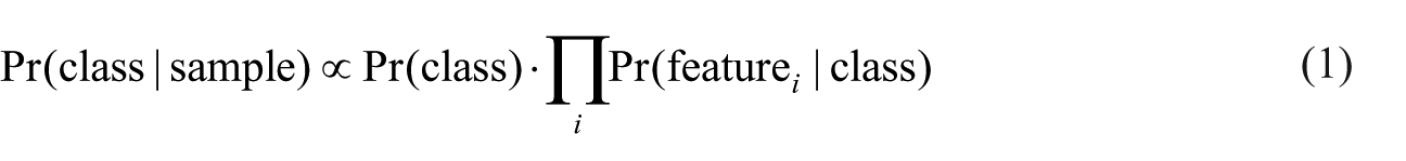
\Pr (class | sample) \propto \Pr (class) \cdot \prod_{i} \Pr ({feature}_{i} | class)

(1)

The NB classifier is very simple and efficient, but it is based on the assumption that all features are independent. This assumption makes the NB classifier a base model used to compare the performance of more complex classifiers.

k-nearest neighbor

k-nearest neighbor (k-NN) is a very popular classification algorithm. It is “instance based” because it does not generate a classification model; classification is achieved by querying the dataset in order to find the closest k samples that are used to infer the class of an observed sample. We used k-NN with k = 9, Euclidean distance and no sample weighting.

Classification tree

A classification tree (CT)¹⁶ is a classifier based on a tree representation of conditions: each non-leaf node in the tree contains a Boolean condition on a feature; on the basis of the truth assigned to the condition, a branch is selected in order to verify the next condition. In the case of a leaf node, a class is assigned. CTs are widely used for classification tasks; however, they suffer from overfitting if not finely tuned. We used a binary CT, with minimum two samples per leaf, subsets are not split if they contain less than five samples and the maximal tree depth is equal to 100.

Random forest

Random forests (RFs) are a combination of CTs identified by a random selection of samples.²² RFs compare well with other ensemble methods and are robust with respect to noise. However, their performance is strictly related to a number of hyper-parameters, which include the number of trees in the forest, as well as pruning strategies. We used RFs of 25 trees with the same configuration of CT.

Support vector machine

A support vector machine (SVM) is a linear classifier that separates the samples with a hyperplane by maximizing the margin between the instances of different classes.²³ The technique often yields supreme predictive performance results, especially in terms of generalization ability. Non-linear classification can be achieved by mapping the original feature space into a new, high-dimensional feature space, through a kernel function. In this work, we used radial basis function (RBF) kernel as it showed the best performance on the available data. We used SVM-C with cost 1.0, tolerance threshold $10^{- 3}$ and maximum 100 iterations.

AdaBoost-SVM

AdaBoost is a meta-algorithm for enhancing the performance of a base machine learning algorithm.²⁴ The output of the base learning algorithms is combined into a weighted sum that represents the final output of the boosted classifier. Subsequent base learners are trained in favor of those instances misclassified by previous classifiers. We used 20 SVMs as base learners, with the learning rate equal to 1.0, and the SAMME algorithm²⁵ for multiclass prediction.

CN2 rule induction

CN2 is an induction method designed for the efficient induction of transparent IF–THEN rules.²⁶ More specifically, CN2 induces an ordered list of classification rules from examples using entropy as its search heuristic. CN2 depends on many parameters: in this work, we used unordered rules, exclusive covering, entropy evaluation and beam width equal to 5 for rule searching, minimum one sample per rule and maximum rule length equal to 5.

The regression models

Mean learner

Mean learner (ML) is the baseline method for regression: it simply returns the mean value of the target, as computed from the training set. ML is used to define the lower performance bound for more complex methods.

Linear regression

Linear regression (LR) is the simplest regression model, which represents the target value as a linear function of the input features. We used the non-regularized version of LR since regularized versions did not give appreciable differences in performance.

k-NN

We used k-NN for regression too. We used $k = 8$ with Manhattan distance and distance weighting of samples.

Regression trees

A regression tree (RT) acts as a CT but leaves contain a numerical estimate of the target. We used RT with the same configuration of CT.

Support vector regression

Support vector regression (SVR) is SVM adapted for regression by appropriately changing the training algorithm. We used a linear SVR, trained with the v-support vector regression (v-SVR)²⁷ algorithm, parametrized by cost equal to 1.0 and complexity bound $(ν)$ equal to 0.5.

AdaBoost-SVR

We applied AdaBoost²⁴ with 50 SVR estimators, linear loss and learning rate equal to 1.0.

Metrics

Metrics for classification

In the case of classification, the performance of a classifier is usually assessed by computing functions on the resulting confusion matrix. In essence, the confusion matrix represents the number $n_{i j}$ (or percentage $p_{i j}$ ) of samples of class $C_{i}$ that have been classified as $C_{j}$ , for varying indexes $i$ and $j$ . In the following, we assume that the number of classes is $c$ and the number of samples is $n$ .

Classification accuracy

Classification accuracy (CA) reports the fraction of samples in the test set which have been correctly classified. For each class $C_{i}$ , the true-positive ${TP}_{i}$ value is the number of samples of class $C_{i}$ that are correctly classified as $C_{i}$ . Then

CA = \frac{\sum_{i} {TP}_{i}}{n}

(2)

Precision

Precision of a class $C_{i}$ is the ratio between ${TP}_{i}$ and the number pred_i of samples classified as $C_{i}$ (irrespective of their actual class). In the case of multiclass problems, the overall Precision is averaged over all classes

Precision = \frac{1}{c} \sum_{i} \frac{{TP}_{i}}{{pred}_{i}}

(3)

Sensitivity (a.k.a. recall)

Sensitivity of a class $C_{i}$ is the ratio between TP_i and the number class_i of samples of class $C_{i}$ . In the case of multiclass problems, the overall Sensitivity is averaged over all classes

Sensitivity = \frac{1}{c} \sum_{i} \frac{{TP}_{i}}{{class}_{i}}

(4)

$F_{1}$ score

The $F_{1}$ score is defined as the harmonic mean between Precision and Recall

F_{1} = \frac{2 \times Precision \times Recall}{Precision + Recall}

(5)

Area under the curve

Area under the curve (AUC) measures the probability that a classifier gives more weight to the right class than to a wrong class. It is defined as the area under a receiver operating characteristic (ROC) curve, which plots the true-positive rate versus the false-positive rate by varying the decision threshold of the classifier. In the case of multiclass problems, the average AUC is considered.

Metrics for regression

The assessment of performance for the regression models is usually performed through some functions on the difference between the target numerical value (AHI) and the value predicted by the model. If $t_{k}$ is the target value and $y_{k}$ the predicted value, then the following metrics are usually adopted.

Mean squared error

Mean squared error (MSE) averages the squared differences between the target and the actual values

MSE = \frac{1}{n} \sum_{k} {(y_{k} - t_{k})}^{2}

(6)

MSE is very sensitive to outliers, that is, rare samples for which the difference between the target and actual values is very high.

Root mean squared error

Root mean square error (RMSE) is simply defined as the square root of MSE

RMSE = \sqrt{MSE}

(7)

RMSE represents the sample standard deviation of the differences between the predicted and observed values.

Mean absolute error

Mean absolute error (MAE) is the average absolute difference between the target and actual values

MAE = \frac{1}{n} \sum_{k} | y_{k} - t_{k} |

(8)

Differently from MSE, MAE is less sensitive to outliers.

$R^{2}$

$R^{2}$ is interpreted as the proportion of the variance in the target variable that is predictable from the model output. It is defined as

R^{2} = 1 - \frac{\sum_{k} {(y_{k} - t_{k})}^{2}}{\sum_{k} {(y_{k} - \bar{y})}^{2}}

(9)

where $\bar{y} = (1 / n) \sum_{k} y_{k}$ .

Cross validation

We are interested in verifying how much a predictive model is able to carry out an accurate response for data samples that have never been observed during training. In order to assess this capability, we adopt a cross-validation strategy, which consists in repeating the training of a predictive model on a training set and assessing its performance on a test set. Both the training and test sets are obtained from the original dataset. In each repetition, the training set and the test set change. In particular, we used 10-fold cross validation, which basically consists in partitioning the datasets in 10 subsets (folds); training and testing are repeated 10 times: at each time, 9 folds out of 10 are used for training and the remaining fold is used for testing (the test set varies over all repetitions). In the case of classification problems, we adopted stratified 10-fold cross validation, which guarantees almost the same class distribution in each fold.

In the case that a resampling technique is used for dealing with class imbalance, such as SMOTE, then it has been applied on the training set only (thus leaving the test set in the original form). In this way, the samples in the test set do not concur in the generation of the synthetic samples, thus avoiding an indirect injection of information of the test samples in the training process.

Results

Feature ranking

In Figure 1, we report the results of feature ranking using the methods reported in section “Feature ranking and selection” and sorted by their average values. All the ranking methods agree on BMI as the most important feature; they also agree that FVC% and FEV₁/FVC are the least important features. Moreover, there is no accordance on the relative importance of all the other features. As a consequence, BMI apart, there is no evidence on the influence of any feature, taken singularly, in determining the severity class. A multivariate analysis is thus mandatory.

Figure 1.

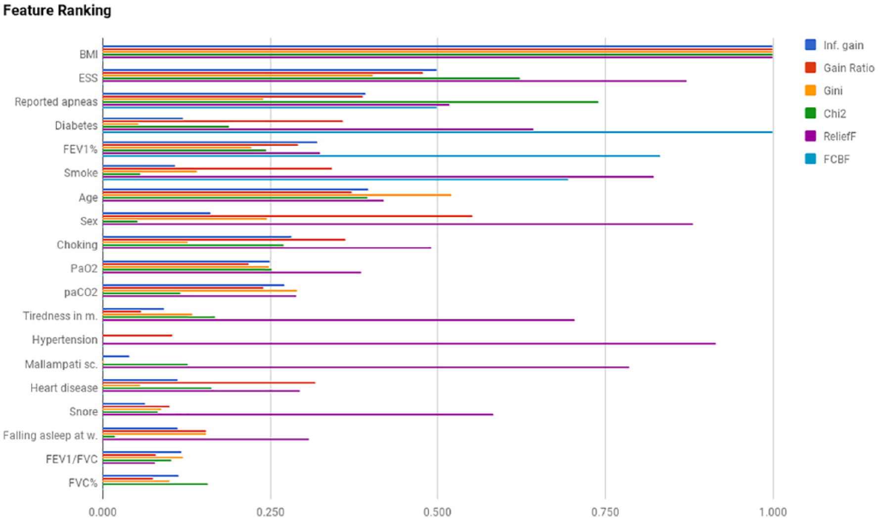
Feature ranking.

Classification results

We applied the considered classification models to the available data, by varying the number of features according to the average ranking provided by the previous analysis. The aim of this approach is to select the minimum number of features that yield the best accuracy values. In fact, by reducing the number of features, we attenuate the risks of overfitting that may hamper the generalization abilities of the classification models. All the classification models have been validated through stratified 10-fold cross validation. We evaluated the classification models under a number of quality metrics, as described in section “Metrics for classification.” For each classification model and a selection of metrics, the average value over the 10 runs of 10-fold cross validation has been computed and is reported in Table 4.

Table 4.

Report of classification metrics for the selected models.

Metrics	SVM (8 feat.)	SVM (3 feat.)	RF (5 feat.)
AUC (%)	65.0	61.7	63.7
CA (%)	44.7	44.7	44.1
$F_{1}$ (%)	41.0	42.0	43.6
Precision (%)	39.9	41.8	44.1
Recall (a.k.a. sensitivity) (%)	44.7	44.7	44.1

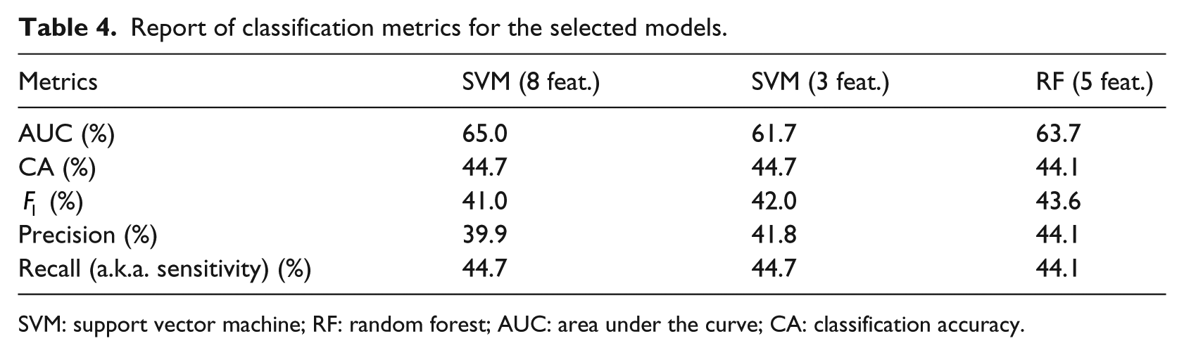
SVM: support vector machine; RF: random forest; AUC: area under the curve; CA: classification accuracy.

The SVM classification model, trained with the first eight features reported in Figure 2, gives the best results in terms of CA and AUC, as quantified in Table 4. A local peak is observed for an SVM with three features, which exhibits similar results in terms of the remaining metrics, with the exception of AUC, which is sensibly smaller.

Figure 2.

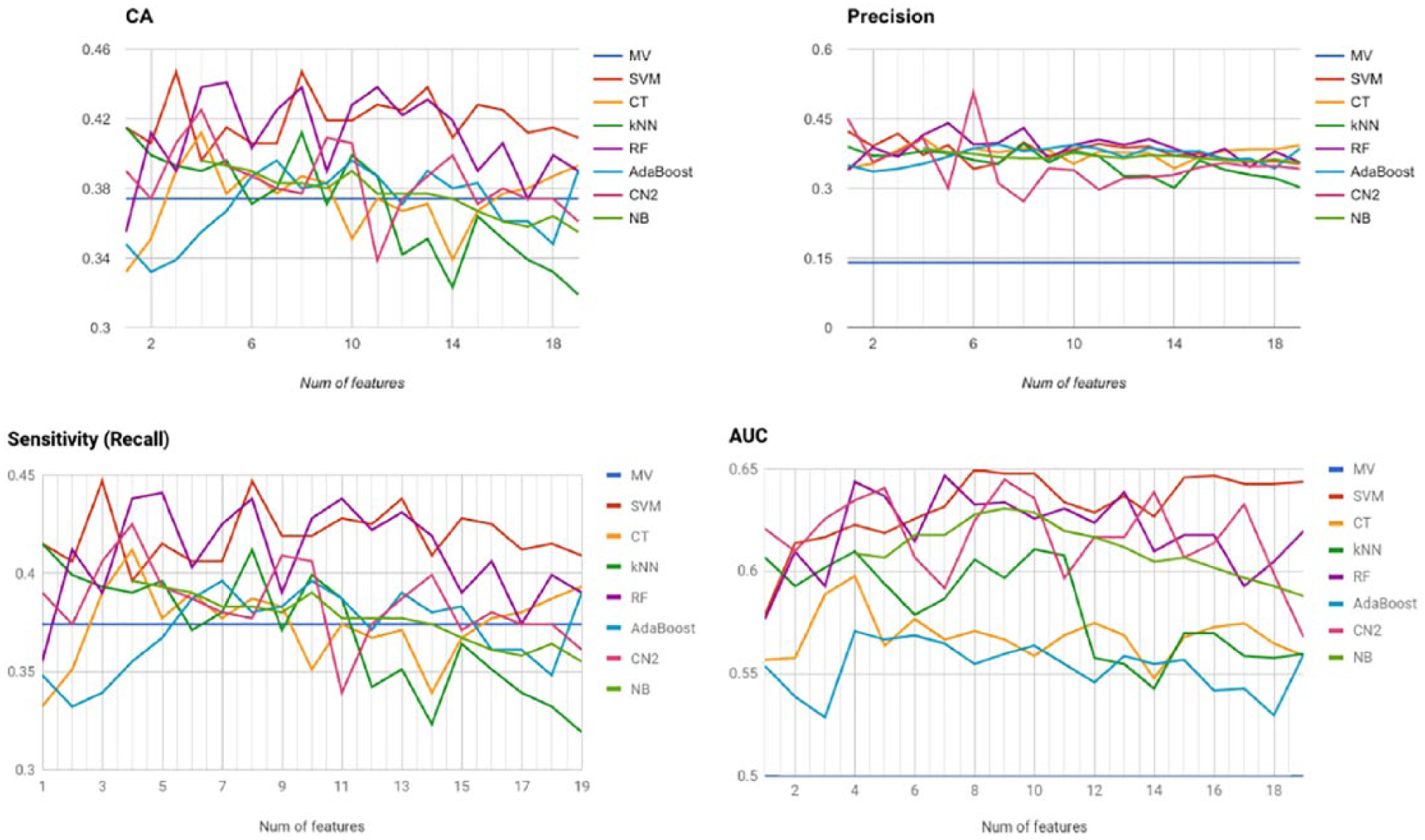
Classification metrics for all models with increasing number of features.

In terms of precision/recall, as synthesized by the $F_{1}$ metrics, the RF classification model—trained with the first five features—shows the best results. In general, RF is more precise than SVM (except when the number of features is too small or too high) and is comparable in terms of recall. This explains the superiority of RF in terms of $F_{1}$ (which is the harmonic mean of precision and recall). However, SVM shows slightly better results in terms of CA.

The remaining classification models do not show relevant results, with the only exception of CN (trained with six features), which exhibits the highest precision value of 50.7 percent. However, it also seems to be a poor classifier in terms of accuracy (38.7%, slightly above the baseline) and recall (38.7%).

In Figure 3, we show the confusion matrices for the selected classification models: SVM (eight and three features) and RF (five features). For the sake of clarity, each row of the confusion matrix shows the distribution frequency of class predictions for all the samples in the test set of a specified class (results are averaged over the 10 runs of 10-fold cross validation).

Figure 3.

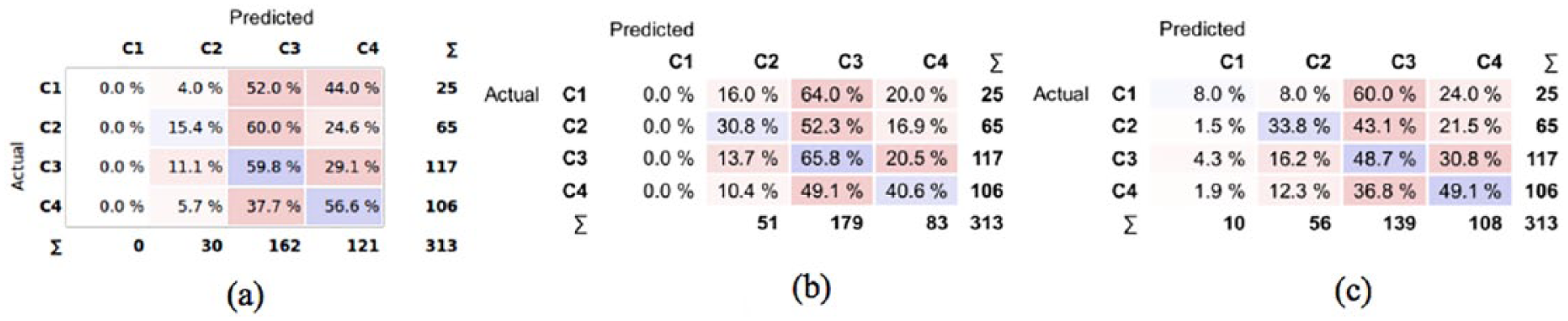
Confusion matrices of the selected models. The values in each matrix represent the percentage of samples of the actual class that are classified in the predicted class: (a) SVM-8, (b) SVM-3 and (c) RF-5.

It is apparent that both SVMs never emit the first class of severity, while RF correctly classifies class 1 samples in only 8 percent of cases. In most cases, class 1 samples are classified with higher levels of severity, which contribute to decrease the CA. However, we are also interested in observing how many samples are assigned a class that is less severe than the actual (this is indeed the worst-case scenario from a clinical viewpoint.) In particular, the most unfavorable condition occurs when a sample of severe class (C4) is predicted as mild (C2) or normal (C1). From Figure 3(a), we see that with SVM-8 this occurs in 5.7 percent of cases (C4 predicted as C2), while the remaining models show significantly higher values. Overall, the SVM trained with eight features shows the best tradeoff in terms of CA, precision, recall and underestimation of OSAS severity.

SMOTE

One of the main sources of difficulty in performing an accurate classification of the available data is the imbalanced distribution of samples in the four classes. The consequences of class imbalance are apparent for the first level of severity (C1), which is represented by about 8 percent of data only. We tried to improve the CA of the selected classification model by oversampling the minority classes through SMOTE. For each fold derived by 10-fold cross validation, we registered the CA of two versions of SVM-8: one trained on the oversampled training set and the other on the on the original data. We tested both models on the same test set (not oversampled). The results are depicted in Figure 4, which does not show a clear superiority of the classification models trained with oversampled data. In fact, according to the Wilcoxon signed-rank test, there is not enough evidence to claim that the population median of differences is different from 0, at the 0.05 significance level. Therefore, we conclude that oversampling is not enough to allow the emergence of a distinctive relation among the selected features, which would have enabled a more accurate discrimination among the four classes.

Figure 4.

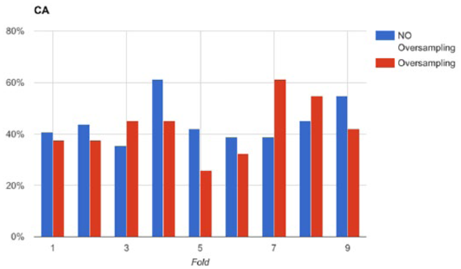
Comparison of classification accuracy along the test sets in a 10-fold cross validation session of SVM-8 with and without SMOTE oversampling.

Regression results

Since the severity classes are obtained by thresholding the AHI feature, we trained a number of regression models on this feature (thus disregarding the severity classes). We generated predictive models trained with an increasing number of features, according to the order derived by feature ranking and reported in Figure 5. We applied 10-fold cross validation (the same folds as for classification) and registered the average values of MSE, RMSE, MAE and R². All these values show the same relations among the selected predictive models, and therefore we report RMSE only in Figure 5. We observe that the best predictive model is SVM-R trained with 16 features (RMSE = 22.17), although there is not a remarkable difference with a different number of features. Also, the performance of SVM-R is comparable with a linear regressor (LR). Furthermore, we observe that the remaining predictive models yields higher values of RMSE (close to the baseline), while RT shows a performance that is always worse than the baseline. Therefore, we conclude that the available data do not give enough information to infer a non-linear relationship between features and AHI, while the linear model exhibits a prediction error that is too high for a reliable prediction of AHI.

Figure 5.

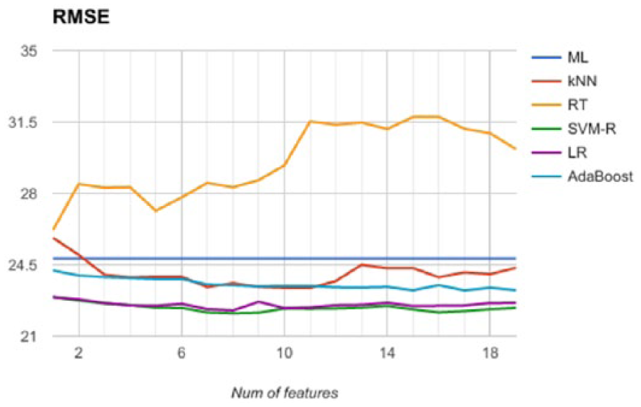
Comparison of the regression models’ accuracy along the test sets in a 10-fold CV session.

Discussion

In this study, we tested the applicability of machine learning methods to predict the severity of OSAS in a population examined in a sleep lab before subjects underwent nocturnal instrumental evaluation. Our work comes from other studies that investigated this issue starting from different points of view and using different analysis approaches. To avoid some problems identified in other works, which generally use a single machine learning method and a relatively small sample, we have applied a complete knowledge discovery process to reduce the limits of previous studies and improve the results obtained by various methods.

First of all, our dataset was built using data from two sleep centers—one in the north and one in the south of Italy—so as to reduce a possible bias induced using the data coming from a single center with the same population. Then, we applied a thorough feature engineering process, based on PCA and feature ranking methods, in order to identify the most suitable set of features that are mostly informative to predict the severity of OSAS. Concerning the design of the predictive models, we adopted two distinct approaches, namely, classification and regression, in order to exploit, as much as possible, the hidden relations between the features and the severity variable. For each modeling approach, we adopted different predictive models that are very popular in Data Science. We also studied the effects of oversampling to deal with the class imbalance observed in the dataset. Finally, we obtained robust prediction results by adopting cross validation for model assessment.

Even if the results are encouraging, from a medical point of view they are not really satisfactory. To achieve our purpose, we followed two different approaches: the first one was to verify if machine learning models can classify the patients with suspected OSAS according to the severity of the disease, while the second approach was to evaluate the ability of models to predict the exact value of AHI. In both cases, the best obtained result is an average of 44.7 percent in terms of CA on test data, too little to say that these methods can turn out as useful tools in routine management of OSAS. Nevertheless, the study allows us to make some considerations on this argument.

First, most studies on OSAS prediction focus on detecting the presence or absence of OSAS. For example, Ustun et al.,²⁸ using supersparse linear integer models, achieved a sensitivity of 64.2 percent and a specificity of 77 percent to predict the presence or absence of OSAS among a population referred to sleep center. Another paper by Su et al.,²⁹ which tested seven different machine learning methods, obtained an accuracy of 84 percent only in one case (multiclass Mahalanobis–Taguchi system), while all other six methods achieved an accuracy much under 65 percent. However, the study reports a validation method based on holdout (66% training, 34% test), which provides less robust results when compared with 10-fold cross validation. Furthermore, this study uses a different set of features for describing the condition of the patients. There is not a standardized procedure for data collection concerning subjects with suspected OSAS and each center uses a custom set of features. This could be a crucial point because the choice of features may influence the results. Future research in this direction is required.

The results of Su et al.²⁹ are substantially in line with those obtained with other tools such as STOP-BANG questionnaire, which achieved a sensitivity of 83.6 percent and a specificity of 56.4 percent, for OSAS defined by AHI > 5.³⁰ Also, a recent meta-analysis performed by Chiu et al.³⁰ compared the use of four different questionnaires (Berlin questionnaire, STOP-BANG questionnaire, STOP questionnaire and ESS) to classify mild, moderate and severe OSAS with respect to AHI (or respiratory disturbance index (RDI)). The authors discovered that, for mild OSAS, the pooled sensitivity levels were from 54 percent to 88 percent with specificity levels ranging from 42 percent to 65 % for moderate OSAS, the pooled sensitivity levels were from 47 percent to 90 percent, with pooled specificity varying from 32 percent to 62 % and for severe OSAS, the pooled sensitivity levels were from 58 percent to 93 percent, with pooled specificity in the range of 28–60 percent. The work confirmed that the sensitivity was higher for STOP-BANG questionnaire with respect to the other test, but also that they had limited value in screening out patients without OSAS.

Our opinion is that these results are influenced by Bayes’ theorem according to which the performance of a screening tool depends on a patient’s pretest probability, or in other words if a test is applied in a low-prevalence setting, the risk of false positives will be low, whereas, when the same test is applied in a high-prevalence setting, the risk of false negatives will be low.

Our population, such as in previous studies, was characterized by a high prevalence of severe and very severe cases of OSAS and low prevalence of mild OSAS, which could justify why our accuracy was higher in the first cases and lower in the second ones. To reduce the influence of this discrepancy, we tried to oversample the mild and moderate cases; however, the result did not change, which may be because there is not sufficient information in the data expressing an implicit relation between features and severity classes, which could have been emphasized by oversampling.

Another interesting consideration regards the definition used to identify the “severity of OSAS.” Each tested system was focused on AHI, which is considered one of the best parameters to estimate the severity of OSAS, especially because it is known that the associations of OSAS and cardiovascular and cerebrovascular morbidity are more evident in subjects with moderate or severe disease.^31,32 We collected data about general parameters, symptoms and comorbidity and tried to find a possible relationship between these data and AHI, but it is also known that there is a dissociation between symptoms and OSAS severity in the particular case of mild and moderate OSAS.³³ Also, even if there is a relationship between OSAS and main comorbidity, there is not a linear correlation between AHI and the presence of comorbidity, especially in some clusters of patients affected by OSAS.³⁴

Feature ranking confirms that BMI and ESS, namely, one parameter related with anatomical characteristics and the other related to symptoms, are the main variables useful to elaborate a predictive model of OSAS severity. Despite this result, which could anyway be influenced by the characteristics of our sample, the weight of these two features for the determination of the severity of OSAS remains low. In fact, as previous studies have demonstrated, the correlation of BMI or ESS with AHI is somewhat variable.³⁴ Thus, it is possible that usual parameters collected to find a mathematical model which can explain the presence and severity of OSAS are not accurate enough to explain the complexity of OSAS. In fact, the onset of OSAS depends on anatomically vulnerable airway and neurologically unstable breathing control, so an accurate model which can predict the severity of OSAS should include different data about these two aspects, and maybe in the future quick screening tools could be elaborated using these data.

Finally, we emphasize the use of stratified 10-fold cross validation to estimate the generalization ability of a predictive model trained from data. Without cross validation, the trained model is likely to be positively biased to a lower classification error due to a hidden overfitting effect. On the other hand, using cross validation, overfitting effects are reduced and a more reliable estimate of the real classification error can be reported.

Limitations

This study presents, in any case, some limitations. We collected our data from two different centers, but we are not able to extend these results to populations from other sleep centers because some data (such as symptoms or comorbidity) may be collected in other ways and in different settings. Besides, we recorded only the presence or absence of some comorbidities except for any data we had about severity of single disease. A standard protocol for data collection in the presence of suspected OSAS is required to acquire as much data as possible and build reliable predictive models based on this information.

Furthermore, the results may have been influenced by the small number of patients with mild diseases. We tried to reduce this bias by oversampling, but this did not yield the expected results due to insufficient sample size.

Finally, another observed limit is on the reduced size of the dataset, especially in comparison with the number of features. In order to overcome this limit, we plan to collect more data from different centers, with the guarantee of uniform description of symptoms, comorbidities and so on.

Conclusion

In order to apply an effective therapy for curing OSAS, an early screening and detection of the syndrome is mandatory. This can be done by classifying patients with possible diagnosis of OSAS into categories according to the severity of the disease, which is a current major research question. Our core objective has been to contribute to these investigations by analyzing and scoring various machine learning algorithms based on respiratory signals and clinical variables instead of the use of full PSG. The discriminating power between normal subjects and sufferers from OSAS has been examined considering different efficacy/efficiency parameters such as accuracy, precision, sensitivity and AUC by means of cross validation.

To our knowledge, this is the first study designed to validate the results of application of machine learning methods in the management of OSAS patients. Our work shows that, at present, the clinical features commonly collected for OSAS patients do not carry the necessary information to make an accurate assessment of OSAS severity with the most widely used machine learning methods. Even if these methods are potentially applicable, there are many drawbacks and we are still far away from their routine use in clinical settings. Nevertheless, the small percentage of severity underestimation suggests that the resulting models could be useful to identify a priority level for assigning patients to the PSG test. To improve the results, these and new methods will be studied with a larger number of subjects but different features are mandatory to evaluate the potentialities of machine learning methods in this field.

Footnotes

Declaration of conflicting interests

The author(s) declared no potential conflicts of interest with respect to the research, authorship and/or publication of this article.

Funding

The author(s) received no financial support for the research, authorship and/or publication of this article.

ORCID iD

Crescenzio Gallo

References

Peppard

Young

Barnet

, et al. Increased prevalence of sleep-disordered breathing in adults. Am J Epidemiol 2013; 177(9): 1006–1014.

Heinzer

Vat

Marques-Vidal

, et al. Prevalence of sleep-disordered breathing in the general population: the HypnoLaus study. Lancet Respir Med 2015; 3(4): 310–318.

McNicholas

Bonsigore

and The Management Committee of EU COST ACTION B26. Sleep apnoea as an independent risk factor for cardiovascular disease: current evidence, basic mechanisms and research priorities. Eur Respir J 2007; 29(1): 156–178.

Kapur

Auckley

Chowdhuri

, et al. Clinical practice guideline for diagnostic testing for adult obstructive sleep apnea: an American Academy of Sleep Medicine clinical practice guideline. J Clin Sleep Med 2017; 13(3): 479–504.

Rowley

Aboussouan

Badr

MS.

The use of clinical prediction formulas in the evaluation of obstructive sleep apnea. Sleep 2000; 23(7): 929–938.

Netzer

Stoohs

Netzer

, et al. Using the Berlin Questionnaire to identify patients at risk for the sleep apnea syndrome. Ann Intern Med 1999; 131(7): 485–491.

Chung

Yegneswaran

Liao

, et al. STOP questionnaire: a tool to screen patients for obstructive sleep apnea. Anesthesiology 2008; 108(5): 812–821.

JV.

Advantages and disadvantages of using artificial neural networks versus logistic regression for predicting medical outcomes. J Clin Epidemiol 1996; 49(11): 1225–1231.

Kirby

Eng

Danter

, et al. Neural network prediction of obstructive sleep apnea from clinical criteria. Chest 1999; 116(2): 409–415.

10.

Sun

Chiu

Chuang

, et al. A prediction model based on an artificial intelligence system for moderate to severe obstructive sleep apnea. Sleep Breath 2011; 15(3): 317–323.

11.

American Academy of Sleep Medicine Task Force. Sleep related breathing disorders in adults: recommendations for syndrome definition and measurement techniques in clinical research. Sleep 1999; 22: 667–689.

12.

Verleysen

Damien

The curse of dimensionality in data mining and time series prediction. In: Cabestany

Prieto

Sandoval

(eds) Computational intelligence and bioinspired systems lecture notes in computer science. London: Springer, 2005, pp. 758–770.

13.

Kuhn

Kjell

Applied predictive modeling. New York: Springer, 2016.

14.

Duch

Wieczorek

Biesiada

, et al. Comparison of feature ranking methods based on information entropy. In: 2004 IEEE international joint conference on neural networks, Budapest, 25–29 July.

15.

Quinlan

. Simplifying decision trees. Int J Man Mach Stud 1987; 27(3): 221–234.

16.

Quinlan

. C4.5: programs for machine learning. Amsterdam: Morgan Kaufmann, 2006.

17.

Liu

Setiono

. Chi2: feature selection and discretization of numeric attributes. In: Proceedings of 7th IEEE international conference on tools with artificial intelligence, Herndon, VA, 5–8 November 2005.

18.

Robnik-Šikonja

Kononenko

Theoretical and empirical analysis of ReliefF and RReliefF. Mach Learn 2003; 53(1–2): 23–69.

19.

Liu

Efficient feature selection via analysis of relevance and redundancy. J Mach Learn Res 2004; 5: 1205–1224.

20.

Chawla

Bowyer

Hall

, et al. SMOTE: synthetic minority over-sampling technique. J Artif Intel Res 2002; 16: 321–357.

21.

Aggarwal

CC.

Data classification: algorithms and applications. Boca Raton, FL: CRC Press, 2015.

22.

Breiman

Random forests. Mach Learn 2001; 45(1): 5–32.

23.

Schölkopf

Smola

AJ.

Learning with kernels: support vector machines, regularization, optimization, and beyond. Cambridge, MA: The MIT Press, 2001.

24.

Freund

An adaptive version of the boost by majority algorithm. Mach Learn 2001; 43(3): 293–318.

25.

Zhu

Zou

Rosset

, et al. Multi-class AdaBoost. Stat Interface 2009; 2(3): 349–360.

26.

Clark

Niblett

The CN2 induction algorithm. Mach Learn 1989; 3(4): 261–283.

27.

Schölkopf

Bartlett

Smola

, et al. Shrinking the tube: a new support vector regression algorithm. In: Proceedings of the 11th international conference on neural information processing systems, Denver, CO, 1–3 December, pp. 330–336. Cambridge, MA: The MIT Press.

28.

Ustun

Westover

Rudin

, et al. Clinical prediction models for sleep apnea: the importance of medical history over symptoms. J Clin Sleep Med 2016; 12(2): 161–168.

29.

Chen

, et al. Prediagnosis of obstructive sleep apnea via multiclass MTS. Comput Math Methods Med 2012; 2012: 212498.

30.

Chiu

Chen

Chuang

, et al. Diagnostic accuracy of the Berlin questionnaire, STOP-BANG, STOP, and Epworth Sleepiness Scale in detecting obstructive sleep apnea: a bivariate meta-analysis. Sleep Med Rev 2016; 36: 57–70.

31.

Gottlieb

Yenokyan

Newman

, et al. Prospective study of obstructive sleep apnea and incident coronary heart disease and heart failure: the Sleep Heart Health Study. Circulation 2010; 122(4): 352–360.

32.

Redline

Yenokyan

Gottlieb

, et al. Obstructive sleep apnea-hypopnea and incident stroke: the sleep heart health study. Am J Respir Crit Care Med 2010; 182: 269–277.

33.

Arnardottir

Bjornsdottir

Olafsdottir

, et al. Obstructive sleep apnoea in the general population: highly prevalent but minimal symptoms. Eur Respir J 2016; 47(1): 194–202.

34.

Lacedonia

Carpagnano

Sabato

, et al. Characterization of obstructive sleep apnea-hypopnea syndrome (OSAS) population by means of cluster analysis. J Sleep Res 2016; 25(6): 724–730.

Application of machine learning to predict obstructive sleep apnea syndrome severity

Abstract

Introduction:

Materials and methods:

Results:

Conclusion:

Keywords

Introduction

Materials and methods

Dataset

Preprocessing

Preliminary feature selection

Feature ranking and selection

Oversampling

The predictive models

The classification models

Majority vote

Naive Bayes

k-nearest neighbor

Classification tree

Random forest

Support vector machine

AdaBoost-SVM

CN2 rule induction

The regression models

Mean learner

Linear regression

k-NN

Regression trees

Support vector regression

AdaBoost-SVR

Metrics

Metrics for classification

Classification accuracy

Precision

Sensitivity (a.k.a. recall)

F 1 score

Area under the curve

Metrics for regression

Mean squared error

Root mean squared error

Mean absolute error

R 2

Cross validation

Results

Feature ranking

Classification results

SMOTE

Regression results

Discussion

Limitations

Conclusion

Footnotes

Declaration of conflicting interests

Funding

ORCID iD

References

$F_{1}$ score

$R^{2}$