Sage Journals: Discover world-class research

Abstract

We utilize deep neural networks to develop prediction models for patient survival and conditional survival of colon cancer. Our models are trained and validated on data obtained from the Surveillance, Epidemiology, and End Results Program. We provide an online outcome calculator for 1, 2, and 5 years survival periods. We experimented with multiple neural network structures and found that a network with five hidden layers produces the best results for these data. Moreover, the online outcome calculator provides conditional survival of 1, 2, and 5 years after surviving the mentioned survival periods. In this article, we report an approximate 0.87 area under the receiver operating characteristic curve measurements, higher than the 0.85 reported by Stojadinovic et al.

Keywords

classification colon cancer outcome calculator Surveillance Epidemiology and End Results

Introduction

Colon and rectum cancers rank among the top cancer types worldwide. The chances of survival increase with early diagnosis, and treatment can greatly increase the chances of eliminating the disease.¹ Colon cancer is common among men than women. The Surveillance, Epidemiology, and End Results (SEER) Program is a good source of domestic statistics of cancer. SEER approximately covers 30 percent of the US population representing different races and across several geographic regions. The data are publicly available through the SEER website upon submission and approval of a SEER limited-use data agreement form.

In this article, we analyze data obtained from the SEER program, in particular, the colon cancer data. Our goal is to develop accurate survival and conditional survival prediction models for colon cancer and making these models publicly available via an outcome calculator. The data analyzed in our study are from SEER’s colon and rectum cancer incidence between 1973 and 2010. The follow-up cutoff date of the data set is 31 December 2010.² These incidences are collected from four different regions in the United States.

Neural networks are considered deep when they have more than two hidden layers.³ Deep neural networks (DNNs) have been successfully used to solve image,^4–6 speech recognition,⁷ and text classification⁸ problems. In this work, we used DNNs to predict survival of colon cancer patients, at the end of 1, 2, and 5 years of diagnosis. We also predict conditional survival given survival of 1, 2, and 5 years. We built models to predict outcomes of colon cancer based on a set of patient attributes. We experimented with multiple neural network structures and found that a network with five hidden layers produces the best results for these data. Moreover, we developed a front end to effectively provide a tool to facilitate user interaction with the developed models. This tool can be used to provide insight from the historical data that SEER provides.

Background

The increase in availability of electronic medical records leads to interest in mining medical data. Data mining research has been published on private hospital data^9,10 and publicly available data such as American College of Surgeons National Surgical Quality Improvement Program (ACS NSIQP)^11,12 and United Network for Organ Sharing (UNOS).^13,14 Since SEER data are publicly available, there have been many studies conducted on its data. SEER provides a tool, SEER*Stat, to assist in generating statistics about their data. Data mining applications have been developed on various types of cancer. Zhou and Jiang¹⁵ explored decision trees and artificial neural networks for survivability analysis of breast cancer. Also, using the breast cancer data, Delen et al.¹⁶ studied neural networks, decision trees, and logistic regression for survivability prediction. Survival of lung cancer on SEER data has been studied by Chen et al.¹⁷ Agrawal et al.^18,19 analyzed SEER lung cancer patients and provided an outcome calculator for survival and conditional survival using ensemble voting techniques.

Data mining applications and studies of colorectal cancer are not covered as much as breast or lung cancers. Fathy²⁰ studied colorectal cancer survival prediction rates versus the number of hidden nodes in the artificial neural networks (ANNs). Stojadinovic et al.²¹ developed a clinical decision support model using Bayesian belief network (ml-BBN). Wang et al.²² analyzed colorectal cancer survival based on different parameters such as stage, age, gender, and race.

The continuous success of deep learning in the fields of computer vision and speech recognition and the increase in availability of electronic health records (EHRs) helped the surge of research of different types of neural networks on EHR. Cheng et al.²³ proposed a convolutional neural network (CNN) to extract phenotypes and perform prediction of chronic diseases on patient EHR. Lipton et al.²⁴ used intensive care unit (ICU) data and evaluated the ability of recurrent neural networks (RNNs) using long short-term memory (LSTM) units to classify 128 diagnoses given in 13 clinical measurements.

Data

We had earlier analyzed colon cancer data from SEER,²⁵ since then new submission has been made by SEER.²⁶ The new data enabled us to experiment with a newer set of features and get better predictive accuracy using deep learning methods, as presented in this article. The cutoff date for the new SEER data was 31 December 2010. The cutoff date is to determine the status of the patient at the time of data release by SEER. If a patient had survived past the cutoff date, but passed away afterward, their status at the cutoff date is the one reported, that is, the patient is reported alive. If a patient was diagnosed after the cutoff date, their record is excluded from the data release. We analyze different periods in our study; as a result, each period has a different end date. For example, if we are to build a model for 1-year survival, we consider patients diagnosed up to the year of 2009. This is to guarantee that all patients had a full year before the cutoff date of 2010. The same logic applies to patients analyzed for 3 years of survival; we consider patients diagnosed up to the year of 2007 (see Table 1) for class distributions.

Table 1.

There is clear imbalance in the two classes of colon survival across most of the years we studied.

Survival	Survived	Did not survive
1 year	138,382	40,114
2 years	115,689	55,242
5 years	75,134	72,510
1 year given 1-year survival	115,689	16,833
2 years given 1-year survival	99,120	27,230
5 years given 1-year survival	65,714	42,091
1 year given 2-year survival	99,120	11,161
2 years given 2-year survival	86,066	18,800
5 years given 2-year survival	57,259	31,001
1 year given 5-year survival	65,714	42,091
2 years given 5-year survival	57,259	74,427
5 years given 5-year survival	37,004	16,452

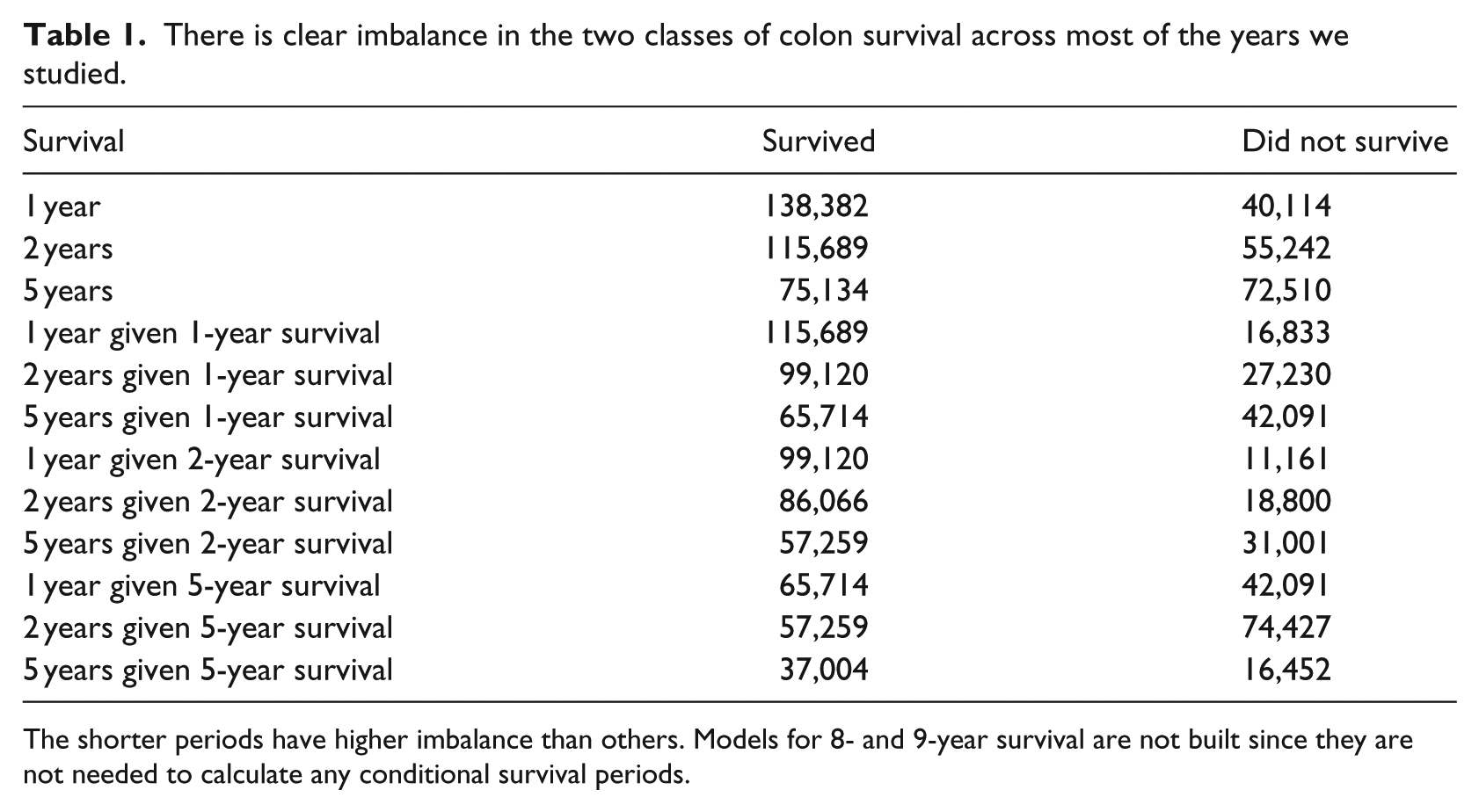
The shorter periods have higher imbalance than others. Models for 8- and 9-year survival are not built since they are not needed to calculate any conditional survival periods.

The majority of features in the data set are categorical features such as sex, birthplace, and stage. A few features are numerical such as tumor size and number of nodes. To overcome this, categorical features were transformed using a one-hot scheme. Each categorical feature was transformed to integers and mapped to sparse matrices where each column corresponds to a category of a feature (see Table 2).

Table 2.

Categorical feature transformation.

X		X_1	X_2	X_3
1		1	0	0
2	→	0	1	0
3		0	0	1
1		0	0	0

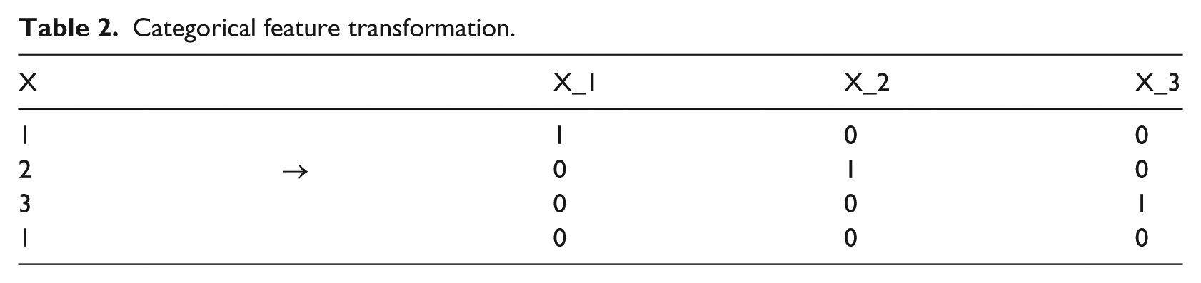
Numerical features were normalized to improve performance of estimators. Standard normalization was applied to numerical features to make such features look more like normal distributions

z = \frac{x - μ}{σ}

(1)

The rest of the article is organized as follows: section “Background” summarizes related work, followed by a description of the data used in this study in section “Data.” A description of the methods used in this work is described in section “Methodology.” Results are presented in section “Results.” In section “Outcome calculator,” a brief description of the outcome calculator is provided, and a conclusion and future work in section “Conclusion and future work.”

Methodology

The SEER data contain attributes that have been collected for specific periods and attributes that contain patient vital status. First, any attributes that contain vital status indication are removed. We combine some attributes such as tumor size. Collaborative Stage (CS) tumor size was collected for years 2004 onward and for years 1988 to 2003 the tumor size was collected under the Extent of Disease (EOD) 10-size feature. A new feature is engineered to cover both periods. After the data are cleaned, they are split into training, validation, and testing (50/30/20). Feature selection is done only from the training set, and the best features are selected from the validation and testing sets based on how their rank was in the training set. DNN models are built using the training and validation sets and then checked against the testing set. Figure 1 gives an overview of the architecture. The following sections describe the components of the system.

Figure 1.

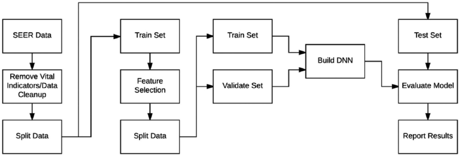
An overview of the steps in our experiment. After the removal of vital status indicators and data cleanup, the data are split into training, validation, and testing sets. Feature selection is performed on the training set and the same features are then selected from the validation and testing sets. Neural network models are built using the training and validation sets and results are reported after running the testing set against the learned models.

Feature selection

The SEER data set have 143 features. In order to build a user-friendly outcome calculator, we need to have a smaller set of features that represents the whole set of features. Any feature that directly indicates the vital status of the patient is manually removed before running feature selection. Using scikit-learn, we select the best performing features on the training set. We use a meta-transformer with a base algorithm of extra-trees. Extra-trees are a set of randomized decision trees on multiple sub-samples of the training data set. The use of randomization and multiple subsets improves accuracy and avoids overfitting. After running the feature selection algorithm, we select features having importance value greater than 0.01. Also, after removing any redundant features, we obtain the features in Table 3.

Table 3.

Features used in building prediction models.

Feature name
Marital status at diagnoses
Race/ethnicity
Year of birth
Birthplace
Grade
Diagnostic confirmation
EOD 10—extension
EOD 10—lymph node involvement
Regional nodes examined
RX Summ—Surg Prim Site
Reason for no surgery
Tumor size
Regional nodes positive
Age at diagnosis

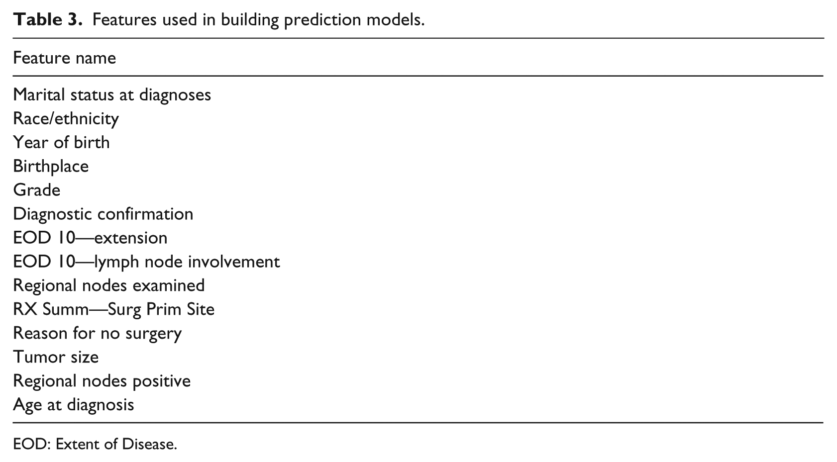
EOD: Extent of Disease.

Neural network building blocks

Rectified linear unit is an activation function that is strictly non-negative and its output has a lower bound of 0 with no upper bound (see equation (2) and Figure 2)

f (x) = \max (0, x)

(2)

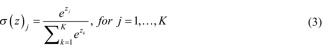
Softmax function is used to transform the outputs of the network into probabilities. It takes an input vector z of length K and outputs a probability vector of the same length that sums to 1²⁷

σ {(z)}_{j} = \frac{e^{z_{j}}}{\sum_{k = 1}^{K} e^{z_{k}}}, f o r j = 1, \dots, K

(3)

Figure 2.

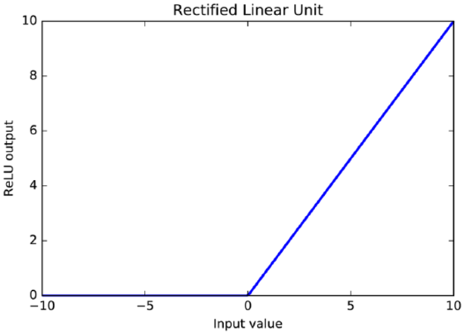
The rectified linear unit activation function is strictly non-negative and its output has a lower bound of 0, but no upper bound. It yields neurons with exactly 0 activation, that is, inputs to the activation function that are below 0 will always output an activation of 0.

DNN

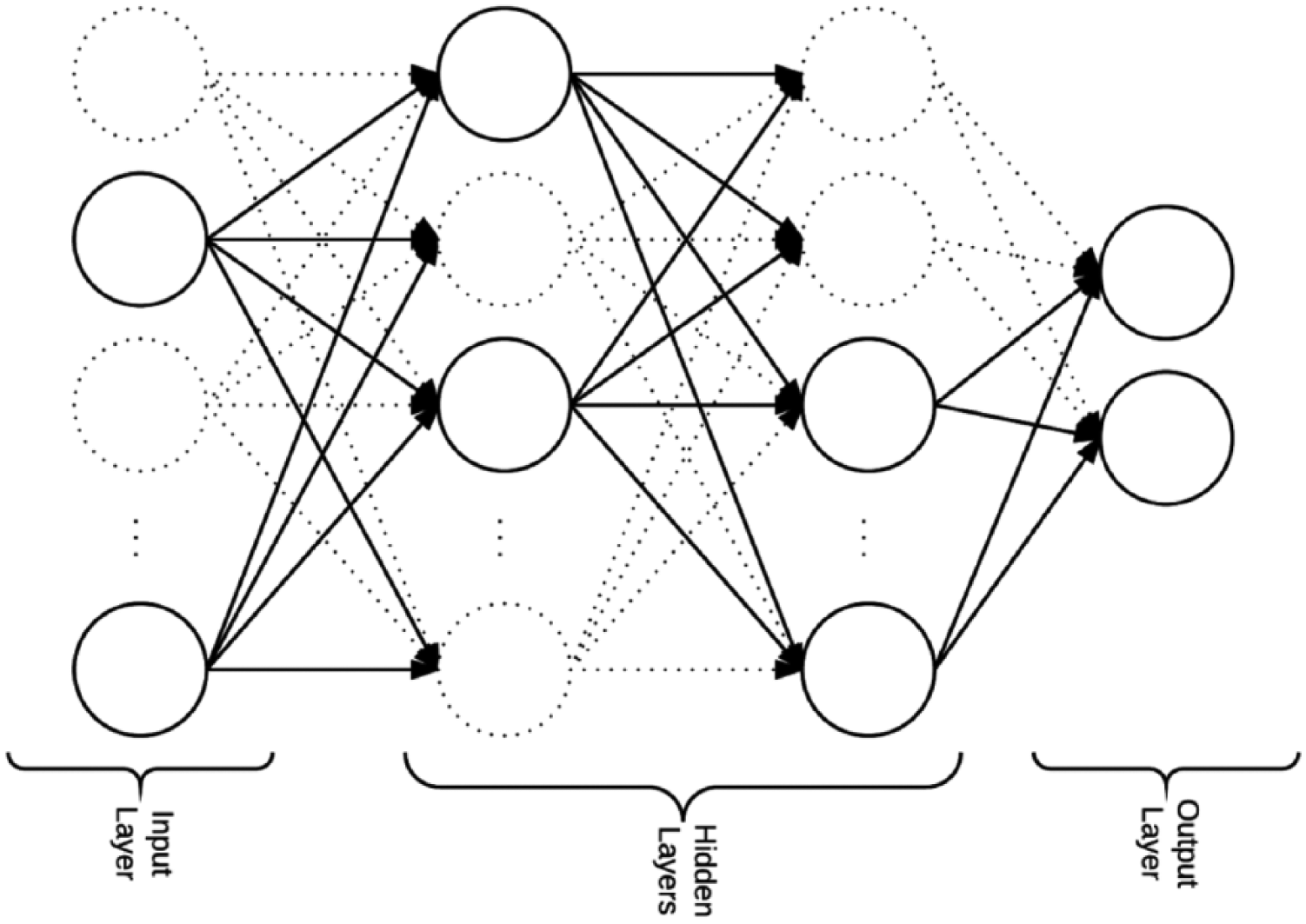
Neural networks are inspired by biological neural networks. They are used to estimate functions based on inputs and weight adjustments for hidden layer nodes “neurons.” These adjustments enable these networks to learn.²⁸ Each node “neuron” has an activation function that defines the nodes output given an input (see Figure 3 for a full connected neural network structure example). All activation functions in the experiments were rectified linear units. A neural network is considered deep if it has more than two hidden layers.³

Figure 3.

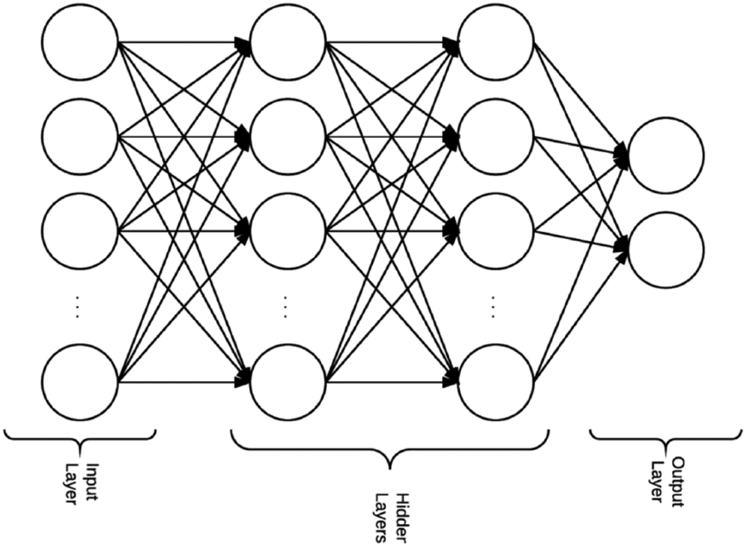
An example of a neural network structure with two hidden layers.

The neural network is trained by performing a forward pass. Then, the error is calculated by comparing the actual class and predicted class. Based on the error, a backward pass is done (backpropagation) to adjust the weights of the network. The neural network is trained on mini-batches randomly sampled inputs from the training set.

Baseline models

We compare the performance of our neural networks approach against two baseline classifiers: random forests and logistic regression:

Random forest. The random forest²⁹ classifier consists of multiple decision trees. The final class of an instance in a random forest is assigned by outputting the class that is the mode of the outputs of individual trees, which can produce robust and accurate classification and ability to handle a very large number of input variables.

Logistic regression. Logistic regression³⁰ is used for prediction of the probability of occurrence of an event by fitting data to a sigmoidal S-shaped logistic curve. Logistic regression is often used with ridge estimators to improve the parameter estimates and to reduce the error made by further predictions.

Conditional survival

Conditional survival is the probability of a patient surviving an additional y number of years after surviving x number of years. We create different data sets to build conditional survival models. For example, to calculate conditional survival of 5 years given that the patient already survived 2 years, we first select patients that have survived 2 years. Then, we mark a patient to be alive if they satisfy surviving a total of 7 years; otherwise, they are marked no alive. The Colon Cancer Outcome Calculator presented here calculates patient-specific survival and conditional survival probabilities.

Artificial neural network structure

Developments packages

The DNNs used in our experiments were developed using TensorFlow³¹ an open-source software library for numerical computation and, Keras³² a minimalist, neural networks library, written in Python. Keras was used to enable fast experimentation with different network structures.

Selecting the network structure

In our experiments, we trained fully connected neural networks. We started by training a single-layer network and captured the performance measures of the network on a test data set. By iteratively adding layers to expand the network, we collected performance measures of networks of depths ranging from a single layer to eight layers. We trained models with depths between one and eight hidden layers. We selected the network consisting of five hidden layers, and our selection was based on the five measures we used to evaluate our models. As shown in Figure 4, the collective set of measures performs best for the neural network with five hidden layers. The DNN structure that we used was selected based on training on 1-year survival data. The same network structure was used on the remaining periods.

Figure 4.

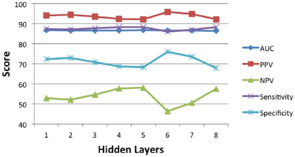
Comparison of all performance measures at different network depths was made to select the best network structure. A network with five hidden layers was selected and used for all survival periods.

Final structure

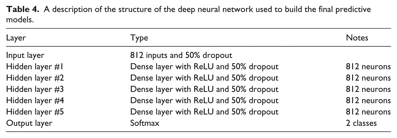
A description of our network is presented in Table 4. Our proposed neural network consists of an input layer, five hidden layers, and a softmax output layer. All of the layers are fully connected dense layers with rectified linear units.

Table 4.

A description of the structure of the deep neural network used to build the final predictive models.

Layer	Type	Notes
Input layer	812 inputs and 50% dropout
Hidden layer #1	Dense layer with ReLU and 50% dropout	812 neurons
Hidden layer #2	Dense layer with ReLU and 50% dropout	812 neurons
Hidden layer #3	Dense layer with ReLU and 50% dropout	812 neurons
Hidden layer #4	Dense layer with ReLU and 50% dropout	812 neurons
Hidden layer #5	Dense layer with ReLU and 50% dropout	812 neurons
Output layer	Softmax	2 classes

Neural network regularization

Two of the useful techniques to regularize the network during training are examining the validation set error after each epoch and dropout implementation.

Early termination

It prevents overfitting of the network by looking at the performance on the validation set and stopping the training of the neural network as soon as the loss stops improving, that is, decreasing in value. Early termination prevents over optimizing on the training set and takes in consideration the validation set. In our experiments, we monitor the validation loss and stop the training when the loss does not decrease over two consecutive epochs.

Dropout

Different layers of the network are connected using activation functions. Dropout is randomly setting a percentage of the activations to 0 during the training of the network (see Figure 5). Dropping out activations enables the network to not rely on specific activations to be present forcing the network to learn redundant representations. These redundant representations make the network robust and avoid overfitting.³³ Moreover, the network acts as an ensemble of networks. In our experiments, we tried training without dropout and dropout out of 25 and 50 percent and found that dropping out 50 percent of the activations gave the best results.

Figure 5.

Randomly dropping out activations enables the network to learn redundant representations. This helps building robust networks and less overfitting.

Performance measures

We use the following performance measures in our experiments to evaluate the DNNs:

Area under ROC curve is a calculation of the area under a curve after plotting the true-positive rate versus the false-positive rate. Since this metric is independent of the classification probability cutoff and truly measures the discriminative power of the model in distinguishing cases from non-cases, it is considered a more reliable evaluation metric than other cutoff-based metrics as described below.

Positive predictive value also known as precision is the ratio of true positives to both true positives and false positives combined and is calculated as follows

P P V o r P r e c i s i o n = \frac{T P}{T P + F P}

(4)

Negative predictive value is the ratio of true negative to both true negative and false negative combined and is calculated as follows

N P V = \frac{T N}{T N + F N}

(5)

Sensitivity is the portion of positive labeled examples in the data set that are classified as positive

S e n s i t i v i t y = \frac{T P}{T P + F N}

(6)

Specificity is the portion of negative labeled examples in the data set that are classified as negative

S p e c i f i c i t y = \frac{T N}{T N + F P}

(7)

Results

We trained multiple models on subset of the SEER data set. The data set of colon cancer patients consists of 188,336 records between the years of 1988 and 2009. All these models were of the same structure presented in Table 4. We compare our results against the results from Stojadinovic et al.²¹ We also show results for conditional survival models in Table 5 and compare the results against the two baseline models we described earlier (random forests and logistic regression).

Table 5.

Result comparison between Bayesian belief network (ml-BBN) model reported by Stojadinovic et al.²¹ and the neural networks (NNs) we developed.

Survival (months)	AUC		PPV		NPV		Sensitivity		Specificity
Survival (months)	BBN	NN	BBN (%)	NN (%)	BBN (%)	NN (%)	BBN (%)	NN (%)	BBN (%)	NN (%)
12	0.85	0.8616	85.1	95.09	74.4	48.29	94.0	86.38	51.4	74.04
24	0.85	0.8675	79.7	90.02	79.9	62.91	90.3	83.56	62.7	75.06
60	0.85	0.8652	64.8	81.91	84.2	72.76	55.5	75.70	88.7	79.51

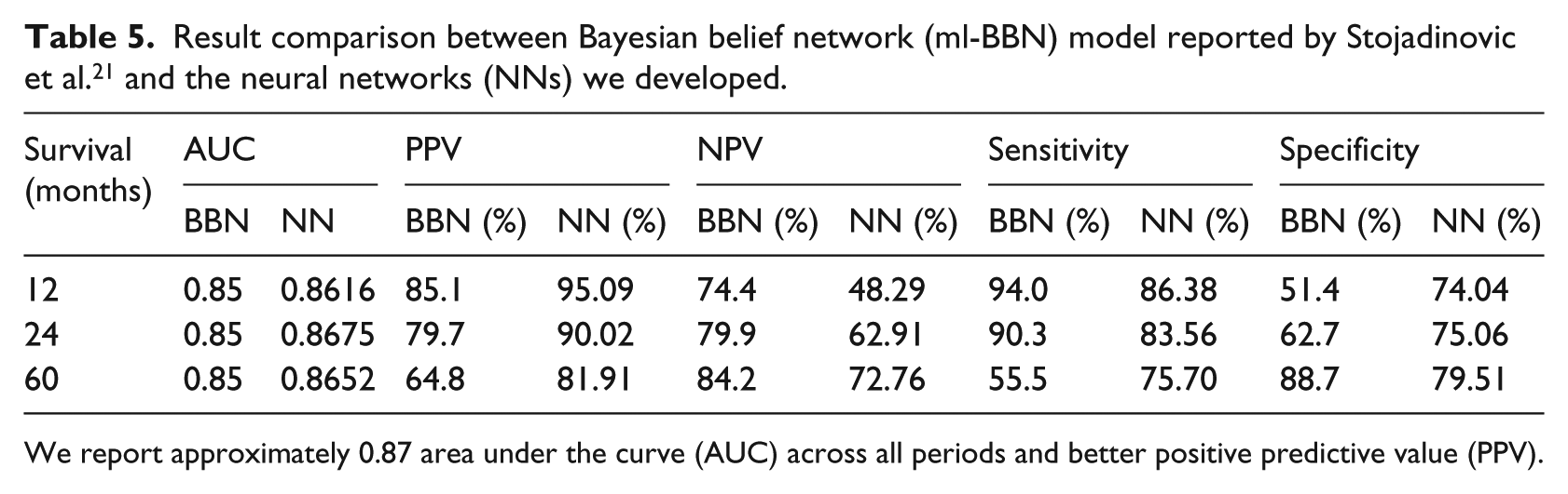
We report approximately 0.87 area under the curve (AUC) across all periods and better positive predictive value (PPV).

Stojadinovic et al. present their results for mortality, whereas our study is for survival. The results are organized accordingly to compare the metrics (see Table 5). Sensitivity measures the proportion of correctly identified positive instances. Our models yield better area under ROC numbers and positive predictive values. Moreover, our models have better specificity percentages for predicting survival for 1, 2, and 3 years. The sensitivity percentages are low due to the imbalance in the two classes (see Table 1 for class distributions). The conditional survival patient distribution is imbalanced and smaller compared to 1, 2, and 5 years data sets, which explains the lower values, specifically area under ROC (Table 6).

Table 6.

Results for the conditional survival models.

Conditional survival	AUC	PPV (%)	NPV (%)	Sensitivity (%)	Specificity (%)
(DNN) 1 year given 1-year survival	0.8090	78.39	66.29	94.11	30.87
(LR) 1 year given 1-year survival	0.8072	97.68	20.94	89.46	56.76
(RF) 1 year given 1-year survival	0.7592	97.43	18.8	89.18	51.55
(DNN) 2 years given 1-year survival	0.8176	74.00	72.77	90.82	43.47
(LR) 2 years given 1-year survival	0.8136	96.21	32.13	83.77	69.97
(RF) 2 years given 1-year survival	0.7799	94.24	33.93	83.85	61.83
(DNN) 5 years given 1-year survival	0.8220	83.30	61.02	76.94	70.06
(LR) 5 years given 1-year survival	0.816	83.73	58.8	76.04	69.83
(RF) 5 years given 1-year survival	0.7872	80.18	58.81	75.24	65.52
(DNN) 1 year given 2-year survival	0.7669	92.06	34.27	92.56	32.69
(LR) 1 year given 2-year survival	0.767	99.15	7.12	90.46	48.62
(RF) 1 year given 2-year survival	0.7074	98.97	6.45	90.38	41.38
(DNN) 2 years given 2-year survival	0.7099	71.23	69.89	91.55	34.67
(LR) 2 years given 2-year survival	0.774	97.68	15.19	84.06	58.81
(RF) 2 years given 2-year survival	0.7363	96.09	16.97	84.12	48.67
(DNN) 5 years given 2-year survival	0.7882	58.60	83.81	86.99	52.29
(LR) 5 years given 2-year survival	0.7806	84.44	49.9	75.69	63.45
(RF) 5 years given 2-year survival	0.7549	82.54	48.44	74.73	60.04
(DNN) 1 year given 5-year survival	0.8629	76.31	49.24	94.93	14.31
(LR) 1 year given 5-year survival	0.7291	99.89	0.09	92.56	6.25
(RF) 1 year given 5-year survival	0.6518	99.67	0.95	92.61	18.52
(DNN) 2 years given 5-year survival	0.7423	69.81	64.92	92.34	26.19
(LR) 2 years given 5-year survival	0.7362	99.44	3.02	86.14	47.11
(RF) 2 years given 5-year survival	0.6831	98.11	5.77	86.32	33.44
(DNN) 5 years given 5-year survival	0.7820	72.22	69.28	84.09	52.58
(LR) 5 years given 5-year survival	0.7744	87.39	42.75	77.44	60.13
(RF) 5 years given 5-year survival	0.7435	85.83	41.72	76.81	56.69

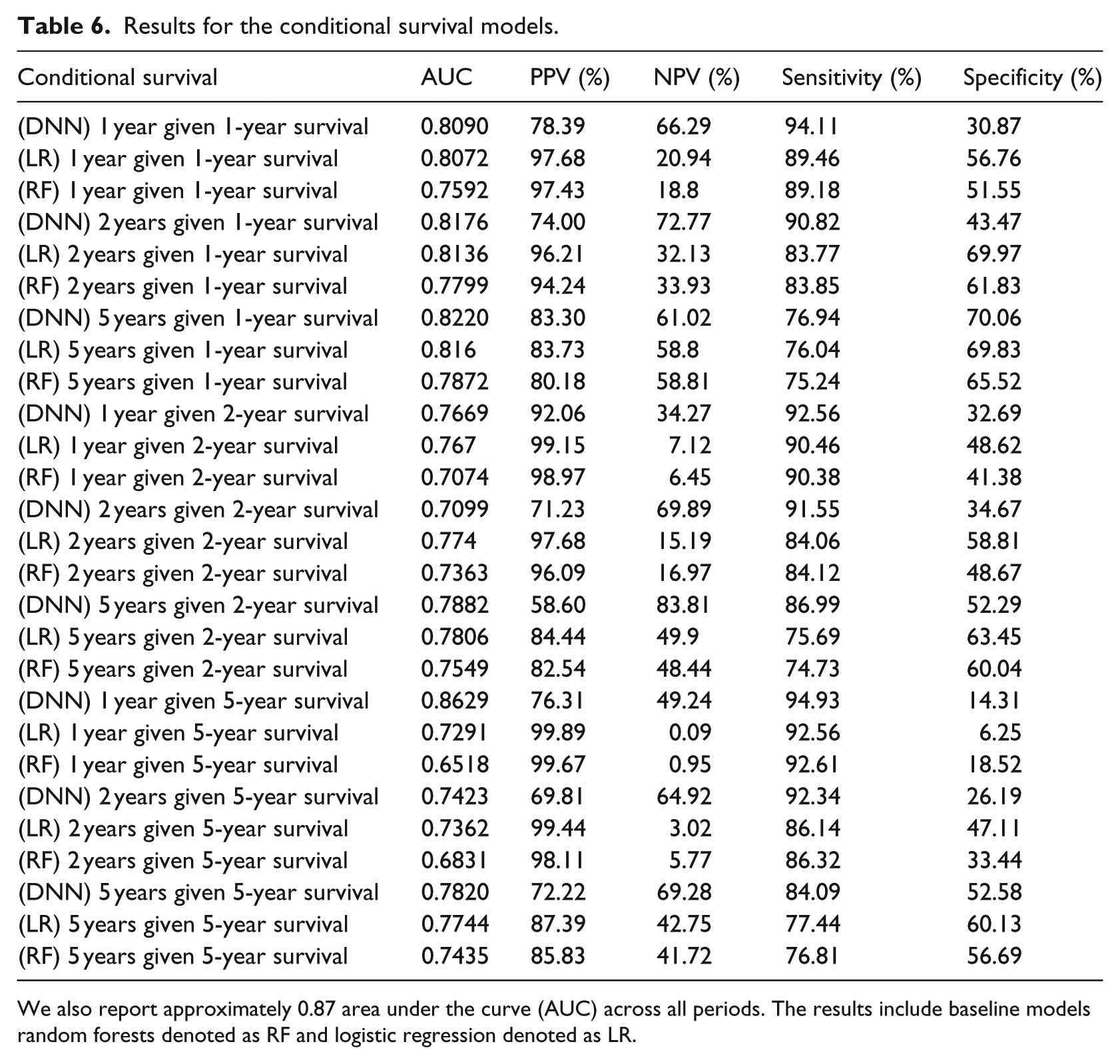
We also report approximately 0.87 area under the curve (AUC) across all periods. The results include baseline models random forests denoted as RF and logistic regression denoted as LR.

Outcome calculator

The purpose of developing an outcome calculator for colon cancer is survival estimation. We used attribute selection techniques to reduce the attribute set. The goal was to have only a few of the attributes to be used in the outcome calculator yet retain comparable production power to the original attribute set. We used 15 attributes in our calculator. Figure 6 shows a screenshot of the outcome calculator.

Figure 6.

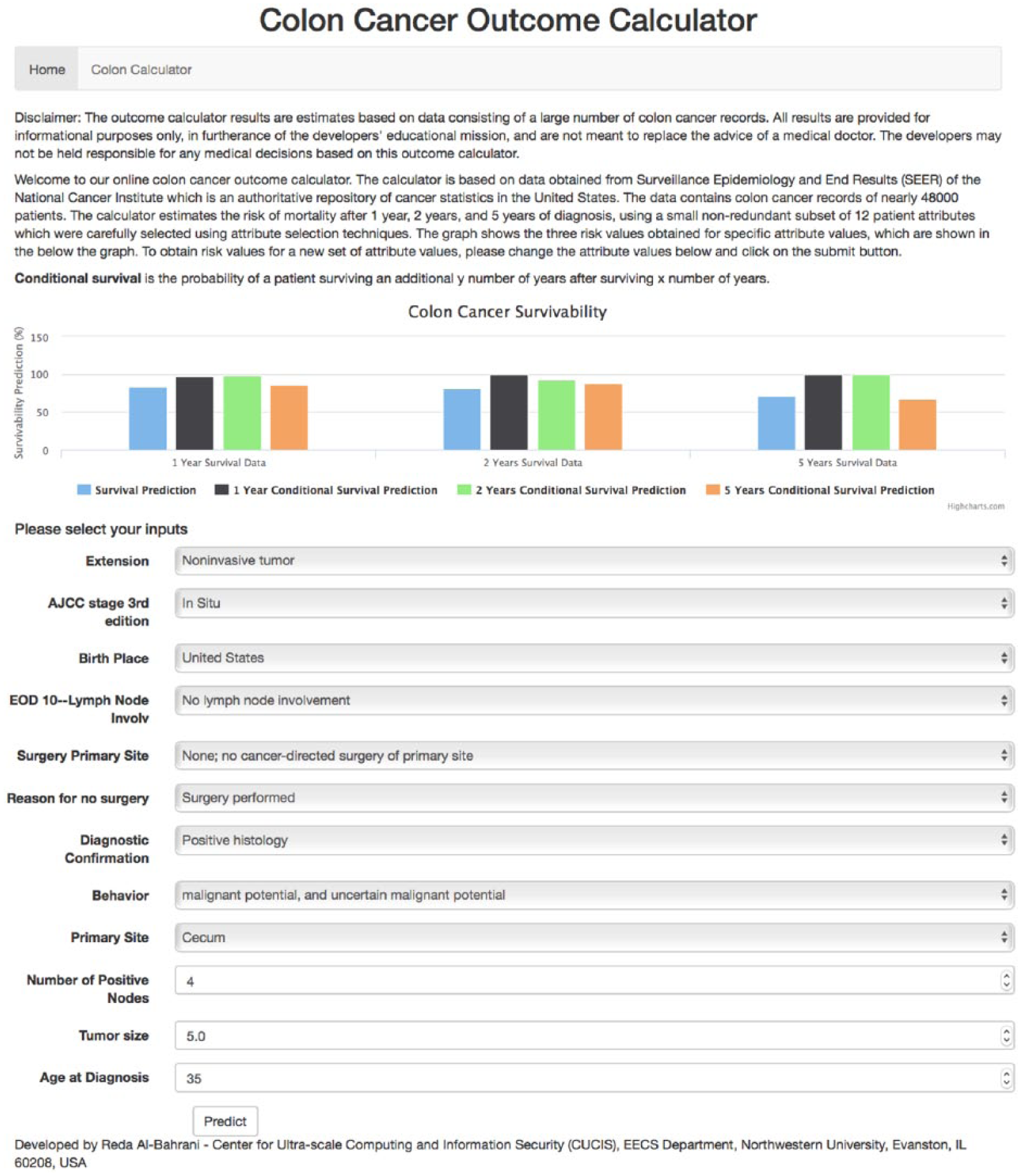
Colon Cancer Outcome Calculator (http://info.eecs.northwestern.edu:5001/).

The outcome calculator was built using several tools: Python,³⁴ Flask,³⁵ Tornado,³⁶ and Apache web server:

Python is a general-purpose programming language. Its strong aspects are code readability and ease of use. It enables concept expression in fewer lines of code than would be possible lower level languages.

Flask is a micro web framework for Python. Applications that use Flask include Pinterest, LinkedIn, and the Flask page.

Tornado is a scalable, non-blocking web server and web application framework written in Python.

Conclusion and future work

In this article, we utilize DNNs to make survival predictions on the SEER program colon cancer data. We look at different depths of neural networks and compare the performance metrics to come up with the best network depth for this problem. We compared our results with a previous study and outperformed in some of the predictive measures. Our models yield better area under ROC numbers and positive predictive values. Our area under ROC numbers for 1, 2, and 5 years of survival were 0.87 compared to 0.85 in the other study. Moreover, our models have better specificity percentages for predicting survival for 1, 2, and 5 years. We compare our models against two baseline machine learning methods: random forests and logistic regression. Although our models have good sensitivity percentages, these could be improved by training on more patient records. Finally, we present our models as a web application for Colon Cancer Outcome Calculator.

For future work, we would like to focus on further improving the neural network architecture, the time it takes to train it, and performance. We could also represent the data with less sparsity and examine whether that helps to improve results. Also, we would like to improve accuracy by training the neural networks on larger data sets. The data set size would be increased by obtaining more data or grouping patients’ records from multiple types of cancer.

Footnotes

Declaration of conflicting interests

The author(s) declared no potential conflicts of interest with respect to the research, authorship, and/or publication of this article.

Funding

The author(s) disclosed receipt of the following financial support for the research, authorship, and/or publication of this article: This work is supported in part by the following grants: NSF award CCF-1409601, DOE awards DE-SC0007456, DE-SC0014330, and Northwestern Data Science Initiative.

References

Parkin

Whelan

Ferlay

, et al. Cancer incidence in five continents, vol. viii. Lyon: IARC Scientific Publications, 2002.

Surveillance, Epidemiology, and End Results (SEER) Program. Research data (1973–2009). National Cancer Institute, DCCPS, Surveillance Research Program, Surveillance Systems Branch released April 2012, based on the November 2011 submission, www.seer.cancer.gov

Winter

and STEUERUNGS-und REGELUNGSTECHNIK. Deep Neural Networks (2012).

Krizhevsky

Sutskever

Hinton

. Imagenet classification with deep convolutional neural networks. In: Advances in neural information processing systems. pp. 1097–1105, https://papers.nips.cc/paper/4824-imagenet-classification-with-deep-convolutional-neural-networks.pdf

Simonyan

Zisserman

. Very deep convolutional networks for large-scale image recognition. arXiv preprint arXiv:14091556. 2014.

Szegedy

Liu

Jia

, et al. Going deeper with convolutions. In: Proceedings of the IEEE conference on computer vision and pattern recognition, Boston, MA, 7–12 June 2015, pp. 1–9. New York: IEEE.

Graves

Mohamed

Hinton

Speech recognition with deep recurrent neural networks. In: 2013 IEEE international conference on acoustics, speech and signal processing, Vancouver, BC, Canada, 26–31 May 2013, pp. 6645–6649. New York: IEEE.

Zhang

Zhao

LeCun

. Character-level convolutional networks for text classification. In: Advances in neural information processing systems, pp. 649–657, https://papers.nips.cc/paper/5782-character-level-convolutional-networks-for-text-classification.pdf

Mathias

Agrawal

Feinglass

, et al. Development of a 5 year life expectancy index in older adults using predictive mining of electronic health record data. J Am Med Inform Assoc 2013; 20(e1): e118–e124.

10.

Liu

Tang

Cheng

, et al. Mining diabetes complication and treatment patterns for clinical decision support. In: Proceedings of the 22nd ACM international conference on information & knowledge management, San Francisco, CA, 27 October–1 November 2013, pp. 279–288. New York: ACM.

11.

Agrawal

Al-Bahrani

Merkow

, et al. Colon surgery outcome prediction using ACS NSQIP data. In: Proceedings of the KDD workshop on data mining for healthcare (DMH), Chicago, IL, 11 August 2013, pp. 1–6. New York: ACM.

12.

Bilimoria

Liu

Paruch

, et al. Development and evaluation of the universal ACS NSQIP surgical risk calculator: a decision aid and informed consent tool for patients and surgeons. J Am Coll Surg 2013; 217(5): 833–842.

13.

Agrawal

Al-Bahrani

Russo

, et al. Lung transplant outcome prediction using UNOS data. In: 2013 IEEE international conference on Big Data, Silicon Valley, CA, 6–9 October 2013, pp. 1–8. New York: IEEE.

14.

Agrawal

Raman

Russo

, et al. Heart transplant outcome prediction using UNOS data. In: KDD workshop on data mining for healthcare (DMH), Chicago, IL, 11 August 2013.

15.

Zhou

Jiang

Medical diagnosis with c4.5 rule preceded by artificial neural network ensemble. IEEE Trans Inf Technol Biomed 2003; 7(1): 37–42.

16.

Walker

Kadam

Predicting breast cancer survivability: a comparison of three data mining methods. Artif Intell Med 2005; 34(2): 113–127.

17.

Chen

Xing

Henson

, et al. Developing prognostic systems of cancer patients by ensemble clustering. BioMed Res Int 2009; 2009: 632786.

18.

Agrawal

Misra

Narayanan

, et al. Lung cancer survival prediction using ensemble data mining on seer data. Sci Program 2012; 20(1): 29–42.

19.

Agrawal

Misra

Narayanan

, et al. A lung cancer outcome calculator using ensemble data mining on SEER data. In: Proceedings of the tenth international workshop on data mining in bioinformatics, San Diego, CA, 21 August 2011, p. 5. New York: ACM.

20.

Fathy

. A prediction survival model for colorectal cancer. In: Proceedings of the 2011 American conference on applied mathematics and the 5th WSEAS international conference on computer engineering and applications, 29 January 2011, pp. 36–42. World Scientific and Engineering Academy and Society (WSEAS), http://www.wseas.us/e-library/conferences/2011/Mexico/CEMATH/CEMATH-03.pdf

21.

Stojadinovic

Bilchik

Smith

, et al. Clinical decision support and individualized prediction of survival in colon cancer: Bayesian belief network model. Ann Surg Oncol 2013; 20(1): 161–174.

22.

Wang

Fuller

Emery

, et al. Conditional survival in rectal cancer: a SEER database analysis. Gastrointest Cancer Res 2007; 1(3): 84–89.

23.

Cheng

Wang

Zhang

, et al. Risk prediction with electronic health records: a deep learning approach. In: Proceedings of the 2016 SIAM International Conference on Data Mining, Jun 30 2016, pp. 432–440. Society for Industrial and Applied Mathematics, https://astro.temple.edu/~tua87106/sdm16.pdf

24.

Lipton

Kale

Elkan

, et al.Learning to diagnose with LSTM recurrent neural networks. arXiv preprint arXiv:151103677 2015.

25.

Al-Bahrani

Agrawal

Choudhary

. Colon cancer survival prediction using ensemble data mining on seer data. In: 2013 IEEE international conference on Big Data, Silicon Valley, CA, 6–9 October 2013, pp. 9–16. New York: IEEE.

26.

Surveillance, Epidemiology, and End Results (SEER) Program. Research data (1973–2011). National Cancer Institute, DCCPS, Surveillance Research Program, Surveillance Systems Branch released April 2014, based on the November 2013 submission, www.seer.cancer.gov

27.

Wikipedia. Softmax function—Wikipedia, the free encyclopedia, https://en.wikipedia.org/w/index.php?title=Softmax_function&oldid=725735236 (2016, accessed 5 August 2016).

28.

Wikipedia. Artificial neural network—Wikipedia, the free encyclopedia, https://en.wikipedia.org/w/index.php?title=Artificial_neural_network&oldid=712077671 (2016, accessed 5 April 2016).

29.

Breiman

Bagging predictors. Mach Learn 1996; 24(2): 123–140.

30.

Friedman

Hastie

Tibshirani

, et al. Additive logistic regression: a statistical view of boosting (with discussion and a rejoinder by the authors). Ann Stat 2000; 28(2): 337–407.

31.

Abadi

Agarwal

Barham

, et al. TensorFlow: large-scale machine learning on heterogeneous systems, 2015, http://tensorflow.org/

32.

Chollet

F. keras

, 2015, https://github.com/fchollet/keras

33.

Srivastava

Hinton

Krizhevsky

, et al. Dropout: a simple way to prevent neural networks from overfitting. J Mach Learn Res 2014; 15(1): 1929–1958.

34.

Wikipedia. Python (programming language)—Wikipedia, the free encyclopedia, https://en.wikipedia.org/w/index.php?title=Python_(programming_language)&oldid=707205791 (2016, accessed 1 March 2016).

35.

Wikipedia. Flask (web framework)—Wikipedia, the free encyclopedia, https://en.wikipedia.org/w/index.php?title=Flask_(web_framework)&oldid=706238434 (2016, accessed 1 March 2016).

36.

Wikipedia. Tornado (web server)—Wikipedia, the free encyclopedia, https://en.wikipedia.org/w/index.php?title=Tornado_(web_server)&oldid=704183715 (2016, accessed 1 March 2016).

Survivability prediction of colon cancer patients using neural networks

Abstract

Keywords

Introduction

Background

Data

Methodology

Feature selection

Neural network building blocks

DNN

Baseline models

Conditional survival

Artificial neural network structure

Developments packages

Selecting the network structure

Final structure

Neural network regularization

Early termination

Dropout

Performance measures

Results

Outcome calculator

Conclusion and future work

Footnotes

Declaration of conflicting interests

Funding

References