Deep ensemble of multi-head attention CNNs for histopathological image-based of lung and colon cancer diagnosis

Abstract

Objectives

Classifying lung and colon cancer from histopathological images remains a significant challenge due to the high degree of intra-class feature similarity and complex tissue morphology, particularly in lung cancer cases. While convolutional neural networks (CNNs) have demonstrated strong spatial feature extraction capabilities, they cannot inherently model long-range dependencies and global contextual relationships. Although attention-based methods partially address these limitations, they often suffer from overfitting, limited generalization across heterogeneous datasets, and insufficient interpretability for clinical adoption. To address these challenges, this study presents a Multi-Head Attention-Based Convolutional Neural Network (MHAB-CNN) ensemble framework that captures localized and global feature interactions critical for robust cancer classification.

Methods

A k-fold cross-validation strategy is adopted to train multiple MHAB-CNN models, from which the empirically top-performing ones are selected and aggregated to form a compact ensemble. This approach improves robustness, reduces overfitting, and ensures computational efficiency. Grad-CAM-based visualizations interpret the discriminative regions influencing the model’s predictions.

Results

Experimental evaluation on the LC25000 dataset demonstrates that the proposed framework achieves an average validation accuracy of 99.84% across folds. Furthermore, the E3 ensemble configuration, comprising models M1, M6, and M9, achieves the highest classification score on the held-out test set.

Conclusion

The proposed MHAB-CNN ensemble framework effectively captures localized and global feature interactions critical for robust lung and colon cancer classification, while improving robustness, reducing overfitting, and enhancing interpretability for potential clinical adoption.

1. Introduction

Around the world, lung and colon cancer are the most widespread and fatal types of cancer. According to the World Health Organization (WHO), in 2022, there were 2.3 million new lung cancer cases, resulting in over 1.8 million deaths. Colon cancer, on the other hand, had about 1.9 million new cases and caused more than 935,000 deaths. ¹ Lung cancer is expected to rank as the leading cause of cancer deaths around the world in the year 2023, with an accelerated trend of 2.5% each year in regions with high rates of smoking and industrial pollution. ² These statistics underscore the urgent need for early diagnosis and effective management of lung cancer, particularly in its initial stages, which are increasingly prevalent and crucial for improving patient survival rates.

Analyzing histopathological images plays a vital role in cancer diagnosis by enabling pathologists to identify and classify malignancies based on abnormal cell morphology, structural patterns, and other pathological indicators. ³ However, this manual diagnostic process presents several challenges. It relies heavily on the expertise and judgment of individual pathologists, which can introduce variability and subjectivity into clinical outcomes. Fatigue, interpretative differences, and the subtlety of certain abnormalities may lead to missed or inconsistent diagnoses. ⁴ Furthermore, the process is time-consuming and labor-intensive, posing significant scalability concerns amid the growing demand for cancer diagnostics. The visual complexity of histopathological patterns often exceeds what can be reliably discerned by the human eye, even experienced professionals. These issues are especially pronounced in resource-constrained settings, where a shortage of trained pathologists leads to further delays in diagnosis and treatment. These challenges collectively underscore the need for advanced technological solutions, particularly artificial intelligence (AI), to enhance cancer diagnosis’s accuracy, efficiency, and scalability.

Machine learning (ML) and deep learning (DL) in medical imaging have significantly advanced diagnostic workflows by offering faster and more accurate analyses. Among various DL techniques, convolutional neural networks (CNNs) have demonstrated exceptional performance, particularly in analyzing histopathological images of lung and colon cancer. ⁵ Although CNNs effectively identify spatial features within images, they exhibit limitations due to their inherent architectural design. A prominent drawback is their inability to model long-range dependencies, as they predominantly capture local spatial relationships and fail to represent global contextual information. ⁶ This limitation can result in incomplete or fragmented interpretations, especially in complex medical images where global coherence is essential. Moreover, CNNs are sensitive to scale, shape, and orientation variations due to their fixed kernel sizes and pooling operations, which restrict their adaptability. They also lack mechanisms to selectively emphasize critical features, potentially leading to noisy or inefficient representations. To mitigate these shortcomings, attention mechanisms ⁷ can be incorporated into CNN architectures,, enabling more nuanced and context-aware analysis of complex and heterogeneous image data.

Attention mechanisms have become a fundamental component of modern DL architectures because they facilitate selective focus on relevant features. Among these, self-attention and its extension, MHA, were first introduced in the transformer architecture. ⁸ Self-attention enables the model to capture dependencies across all positions in the input, irrespective of distance, making it highly effective for representing global context. MHA enhances this capability by employing multiple parallel attention heads, each learning to focus on different input aspects. This parallel processing results in a richer and more expressive representation of the data. ⁹ Following the success of MHA in natural language processing, domain-specific attention mechanisms were proposed to address the unique needs of computer vision tasks. Notably, spatial attention ¹⁰ and channel attention ¹¹ were developed to highlight important regions and informative feature maps in an image, respectively. While these methods have shown improvements in CNNs, they primarily operate within localized scopes and cannot model long-range dependencies. In contrast, MHA captures global relationships and feature interactions across the entire input, making it particularly advantageous for analyzing complex and diverse data, such as histopathological images.

The unique morphological characteristics of lung and colon cancer histopathological images further emphasize the suitability of Multi-Head Attention (MHA) as a foundational mechanism in diagnostic modeling. These images typically exhibit complex spatial configurations, heterogeneous tissue textures, and subtle variations in nuclear structure and glandular formation.^12,13 Such fine-grained patterns, often dispersed across spatially distant regions, pose a significant challenge to traditional CNNs that rely on local feature extraction. ¹⁴ In contrast, MHA enables simultaneous attention to multiple image regions, capturing long-range dependencies and contextual cues for distinguishing between benign, malignant, and pre-malignant tissue subtypes. This capability is critical given the high inter-class similarity among cancer subtypes in both lung and colon tissue, where visual differences can be minimal and easily overlooked. MHA has demonstrated effectiveness in such contexts by improving focus on the most discriminative features while suppressing irrelevant regions. For instance, Wen et al. ¹⁵ leveraged MHA to enhance facial expression recognition by reducing distraction from non-informative areas. Similarly, Sun et al. ¹⁶ showed that MHA facilitates the identification of multiple salient parts within objects, leading to better class separation in visually similar categories. An et al. ¹⁷ introduced a repulsive loss function to diversify attention heads, encouraging the model to capture distinct and complementary features. These strategies are particularly valuable when applied to histopathological classification, where nuanced structural cues must be captured to achieve diagnostic reliability.

Although MHA significantly improves model expressiveness and classification accuracy, its flexibility and depth may increase the risk of overfitting, especially when limited training data. This concern is particularly relevant in medical domains where high-quality annotated datasets are scarce.^18,19 While both CNN and attention-driven strategies have shown promise, their practical implementations in recent studies expose critical limitations in accuracy, generalizability, and interpretability.

For instance, Hasan et al. ²⁰ proposed a lightweight multi-scale CNN to reduce parameter count while maintaining classification performance, and Al-Jabbar et al. ²¹ employed hybrid CNN architectures to improve sensitivity and accuracy. Building further, attention-based mechanisms have also been explored to overcome the locality limitations of traditional CNNs. Provath et al. ²² incorporated attention into CNNs, reporting enhanced diagnostic performance. Despite these improvements, several persistent challenges remain, including vulnerability to overfitting,^18,19 excessive computational burden, ²³ poor generalization to diverse datasets, ²⁴ and lack of interpretability essential for clinical adoption. ²⁵ Moreover, current attention-based models often underutilize ensemble learning strategies, which could otherwise enhance reliability and robustness. ²² To address current shortcomings, we suggest a new approach to ensemble learning that integrates CNNs with Multi-Head Attention MHA to improve the classification processes of lung and colon cancers from histopathological images.

Most current ensemble techniques in analyzing histopathological images are based on output synthesis from different architectures (e.g., VGG, ResNet) using simple averaging or voting. These methods are unfocused on model performance in ensemble formation and lack fold-based training.^26,27

Traditional ensemble techniques, including bagging, stacking, and snapshot ensembles, often feature all models, regardless of the model’s performance, which deteriorates overall performance.^28,29 Additionally, applying interpretable tools such as Grad-CAM, which are mainly focused on individual models, suffers from ensemble effects. ³⁰

Oppositely, our approach has a uniform MHAB-CNN architecture trained in 10 folds, and only the top-3 models based on validation accuracy are selected to construct the ensemble. This selection technique improves model integration because weaker models are excluded, enhancing generalization and robustness. Model interpretability is also advanced at the ensemble level through Weighted and Intersection Grad-CAM heatmaps, strengthening knowledge in this domain. While attention mechanisms address the spatial locality constraints of CNNs, their complexity often increases the risk of overfitting, particularly in limited-data regimes common in medical imaging. To counter this, our approach incorporates a k-fold cross-validation strategy to train multiple lightweight CNN-MHA models, from which the n top-performing models are selected and aggregated. This ensemble strategy enhances predictive reliability, captures complementary representations, and reduces computational overhead by limiting the ensemble size. We conduct comprehensive ablation studies to optimize the number of attention heads used within each model to ensure a trade-off between performance and efficiency. Moreover, advanced visualization techniques are employed to qualitatively assess the discriminative capacity of individual models in the ensemble. The key contributions of this work are as follows:

• We propose a novel and lightweight ensemble learning framework that integrates CNNs with MHA mechanisms to effectively capture spatially diverse and morphologically complex patterns in histopathological images. This combination enhances the model’s capability to discern fine-grained tissue characteristics across long-range dependencies, which is particularly vital in cancer subtype differentiation.

• To mitigate overfitting and improve model generalization, especially in data-scarce medical settings, we employ a k-fold cross-validation scheme and construct an ensemble from the empirically top n performing CNN-MHA models. This strategy balances diversity and computational efficiency, ensuring that only the most robust models contribute to final inference.

• We conduct extensive ablation studies to identify the optimal number of attention heads used within each MHA-augmented CNN. This analysis ensures the ensemble achieves a desirable trade-off between classification accuracy and computational cost, a critical requirement for practical deployment in clinical environments.

• We employ Grad-CAM-based visualization techniques to qualitatively interpret the decision-making behavior of each model in the ensemble. This analysis enables a deeper understanding of the learned feature representations and provides insight into how the ensemble generalizes across diverse histopathological patterns.

• Experimental results on lung and colon histopathological image datasets demonstrate the effectiveness of the proposed framework. The model achieved an average validation accuracy of 99.84% across 10-fold cross-validation, indicating strong and consistent performance. Furthermore, the ensemble achieved a 100% classification accuracy on the held-out test set, highlighting its generalization capability.

The rest of the paper is organized as follows. Section 2 presents the Related Works associated with our work. Section 3 represents the Methodology of the proposed work. Result and Discussion associated with the work is presented in Section 4 and Section 5, respectively. Finally, we present the Conclusion in Section 6.

2. Related Works

Lung and colon cancer classification using histopathological images has gained considerable attention in recent years, leveraging advanced deep-learning architectures, ensemble learning techniques, and optimization methods. Below, we provide a detailed review of key studies in this domain.

2.1. CNN based

Several recent works on lung and colon cancer diagnosis use CNN-based architectures with distinct design strategies that balance accuracy, interpretability, and computational efficiency. For example, Hasan et al. ²⁰ proposed a lightweight multi-scale CNN (LW-MS CNN) that contains only 1.1 million parameters for the classification of lung and colon cancers with a multi-class prediction accuracy of 99.20%. The addition of explainable AI tools, Grad-CAM and SHAP, strengthened the interpretability and trustworthiness of the model. Although best suited for real-time applications, the light nature may also hinder grip over complicated patterns in heterogeneous datasets.

In a parallel direction, Al-Jabbar et al. ²¹ designed hybrid architectures that integrated characteristics of GoogLeNet and VGG-19 networks to perform lung and colon cancer detection with better sensitivity (99.85%) and accuracy (99.64%). While their approach achieved appreciable success, additional experimental refinements did not bring about any substantial improvements. Additionally, the sophistication of the hybrid structure raised issues regarding its practicality and upkeep, indicating that it might be helpful to consider less complicated structures while adopting hybrid systems. Complementing these efforts, Gowthamy and Ramesh et al. ²⁴ are the first to use a hybrid technique combining pre-trained deep learned features with Kernel Extreme Learning Machines for classification. The model has a good trade-off between accuracy and resource usage; the claimed accuracy is 98.9%, and the F1 score is 97.6% and above. Nevertheless, pre-trained models constrain their applicability to different data distributions, and thus are degenerative in their performance (Table 1).

Table 1.

Summary of methods and limitations in lung and colon cancer classification studies.

Paper	Year	Method	Weakness
Sünnetci and Alkan 31	2022	ML with Bag of Features, LDA, SVM, KNN, and probabilistic majority voting	Only applied to lung cancer; not generalized to colon cancer
Talukder et al. 26	2022	Deep feature extraction + ensemble learning	High complexity, scalability concerns, needs optimization
Provath et al. 22	2023	Global context attention-based CNN	No ensemble used; limits robustness and generalization
Mengash et al. 32	2023	Marine Predators Algorithm + MobileNet + DBN	Outcome instability due to heuristic optimization dependency
Al-Jabbar et al. 21	2023	Hybrid GoogLeNet + VGG-19	Complex structure, minimal gains from further refinements
Indumathi and Siva 33	2024	Hybrid CNN-BiLSTM with multi-head self-attention	High computational complexity, limiting real-time clinical use
Abd El-Aziz et al. 23	2024	Fusion of ResNet-101V2, NASNetMobile, EfficientNet-B0	High computational demand; challenging for deployment
Hasan et al. 20	2024	Lightweight Multi-Scale CNN (LW-MS CNN)	Lightweight design may struggle with heterogeneous data
Razmjouei et al. 3	2024	Two-stage ensemble with metaheuristics	Requires extensive hyperparameter tuning; low interpretability
Gowthamy and Ramesh 24	2024	Pre-trained DL + Kernel Extreme Learning Machines	Dependent on pre-trained models; poor generalization on new data
Syal et al. 25	2024	Ensemble-based detection model	Lacks explainability, which is vital for medical settings

2.2. Attention Based Method

Beyond standard convolutional models, attention mechanisms have also been incorporated to enhance feature representation and contextual learning in cancer diagnosis. Provath et al. ²² proposed a global context attention-based convolutional neural network, achieving an impressive image-level accuracy of 99.76% and patient-level accuracy of 96.5%. The model also reduced computational complexity, making it suitable for mobile deployment. However, the lack of ensemble methods limits their potential for improved robustness and generalization.

Similarly, Indumathi and Siva ³³ introduced a hybrid CNN-BiLSTM model with a multi-head self-attention mechanism for predicting lung disorders using medical imaging datasets, achieving high classification accuracies of 94.9%, 97.8%, 97.9%, and 94.6% on the Chest X-ray, PET/CT, CECT, and JSRT datasets, respectively. Despite its superior performance compared to existing models, the computational complexity may hinder its real-time applicability in clinical environments.

2.3. Ensemble based learning

Ensemble-based approaches have also gained traction for cancer diagnosis, aiming to improve robustness, accuracy, and generalization by integrating multiple models or learning strategies. Sünnetci and Alkan ³¹ proposed an automated lung cancer diagnosis framework using machine learning algorithms, probabilistic majority voting, and optimization techniques. The method utilized Bag of Features for feature extraction and employed Linear Discriminant, Optimizable Support Vector Machine, and Optimizable K-Nearest Neighbor classifiers, achieving an accuracy of 99.28%. A detailed theoretical framework for majority voting was provided, and a user-friendly graphical interface was developed to aid radiologists. However, the study was confined to lung cancer detection and did not explore extending the approach to other cancer types, such as colon cancer.

Expanding the coverage to multi-class classification, Abd El-Aziz et al. ²³ proposed a deep learning fusion model for multi-class lung and colon cancer classification. The model combines three pre-trained architectures: ResNet-101V2, NASNetMobile, and EfficientNet-B0, thereby leveraging feature fusion to boost classification accuracy. Therefore, it stands out with exceptional performance metrics, such as 99.94% accuracy on the LC25000 dataset. However, the reliance on multiple Convolutional neural networks (CNNs) increased computational demands, posing challenges for deployment in resource-constrained environments.

Mengash et al. ³² introduced the MPADL-LC3 approach, combining the marine predators algorithm with deep learning to classify lung and colon cancer. The supplementary preprocessing of this approach is based on CLAHE to augment contrast in images; then, feature extraction is performed by MobileNet, and classification by deep belief networks DBN. Hyperparameters were optimized using MPA, which thus increased the performance of the model to an accuracy of 99.27%. However, since it relied on a heuristic optimization algorithm, MPADL-LC3 could have volatile outcomes depending on parameter settings.

Talukder et al. ²⁶ provide a hybrid ensemble model for cancer detection. The authors combine deep feature extraction with ensemble learning, achieving very accurate detection results using the ensemble technique to improve predictive performance. The model’s effectiveness is tested on the LC25000 lung and colon cancer dataset, detecting accuracies of 99.05% lung cancer, 100% colon cancer, and 99.30% combined lung and colon cancer. Nevertheless, computational complexity in merging several ensemble techniques hinders scalability while pointing to optimization that may enhance efficiency and applicability in clinical settings.

Razmjouei et al. ³ proposed a metaheuristic-based two-stage ensemble deep learning architecture to classify lung and colon cancers, thereby obtaining remarkable accuracies of 99.85% on two-class colon cancer and 98.96% on combined lung/colon cancer. However, hyperparameter sensitivity requires extensive tuning, which the model cannot generalize to different datasets. Moreover, multiple CNNs with ML models add non-interpretability; hence, it becomes difficult to justify what led the model to make a particular decision. This opacity is a major hindrance to its use in medical diagnosis.

Syal et al., ²⁵ in a bid to improve the detection of lung and colorectal cancer, came up with an ensemble technique. The model was reliable and resulted in an accuracy of 0.96 percent. However, the paper does not provide specific explainability, which is a critical aspect in medical uses.

Unlike previous works that individually focused on CNNs, attention modules, or ensemble strategies, our proposed framework unifies these components into a single lightweight and interpretable system designed specifically for histopathological cancer diagnosis. While many earlier methods either lacked generalization across cancer types, introduced excessive computational overhead through complex ensemble combinations, or ignored interpretability aspects, our model addresses all three challenges simultaneously. By integrating MHA into compact CNN backbones, selecting top-performing models via k-fold validation, and employing Grad-CAM-based visual explanations, we ensure both high accuracy and transparency. Furthermore, the framework consistently performs well across validation folds and achieves perfect accuracy on the test set, demonstrating strong robustness and practical applicability in clinical scenarios.

3. Methods

The methodology adopted in this research is designed to systematically address the classification of lung and colon cancer using the LC25000 dataset. ³⁴ The overall workflow, illustrated in Figure 1, outlines the key steps involved in the process, from data collection and preprocessing to model training, ensemble creation, and evaluation. Each major step in the workflow is detailed in the subsequent subsections, ensuring a clear understanding of the approach.

Figure 1.

Workflow of the proposed framework with multi-head attention-based CNN.

The workflow begins with collecting and preprocessing the data, including shuffling and splitting it into training and testing subsets. A fixed portion of the data is kept as an independent held-out test set, while the remaining data are used for training and validation. The training subset is further utilized for 10-fold cross-validation to train multiple instances of the proposed MHAB-CNN model. Models with the best validation performance are selected and combined into ensembles using mean and voting strategies to enhance classification reliability. These ensembles are then evaluated on the independent held-out test set to assess their performance. To further ensure interpretability, Grad-CAM visualizations are applied, highlighting the robustness and clarity of the proposed approach. Algorithm 1, outlines the workflow of a MHA-based CNN model, incorporating dataset splitting, k-fold cross-validation, ensemble creation, testing, and Grad-CAM visualization. The following sections elaborate on each of these steps, providing a comprehensive view of the methodology.

3.1. Dataset description

The LC25000 dataset ³⁴ contains twenty-five thousand histopathological images that are uniformly divided into five categories. Each class includes 5,000 samples of composite lung and colon tissues, both healthy and cancerous. This balanced dataset guarantees equal contributions and, therefore, solid, non-biased training and assessment of models developed for classification purposes. Further description of the dataset is provided in Table 2, while Figure 2 exhibits a sample image for every class.

Table 2.

Class-wise sample distribution in the LC25000 dataset.

Class name	Number of samples
Colon Adenocarcinoma (Co_aca)	5,000
Benign Colonic Tissue (Co_n)	5,000
Lung Adenocarcinoma (Lu_aca)	5,000
Benign Lung Tissue (Lu_n)	5,000
Lung Squamous Cell Carcinoma (Lu_scc)	5,000
Total	25,000

Figure 2.

Sample images from the dataset, LC2500.

3.2. Data preprocessing

Several preprocessing steps were applied to prepare the dataset for training. First, all images were resized to a consistent dimension of 224 × 224 pixels. This ensures that every image has the same size, making them compatible with the model’s input requirements. Next, all images were converted to RGB format, ensuring they have the same color structure, regardless of their original format. The images were then transformed into tensors, scaling their pixel values to the range [0, 1], which is essential for efficient processing by the deep learning model. Additionally, labels were assigned to each image based on the folder structure of the dataset. Each class was mapped to a unique numerical value, making it easier for the model to understand and differentiate between the categories during training.

3.3. Dataset splitting and cross-validation

The dataset is partitioned into training and testing sets, ensuring class balance in both splits (Figure 3). Specifically, 10% of the data (with each class contributing 2% of the total samples) is set aside as the test set for final evaluation. The remaining 90% of the data (with each class contributing 18% of the total samples) is used for training. To ensure a thorough and reliable model evaluation, the training set undergoes 10-fold cross-validation, where it is evenly divided into 10 folds, with each fold serving as a validation set in turn while the others are used for training. For example:

• In the first fold (F₁), fold 1 is used for validation, and folds 2 through 10 are used for training.

• In the last fold (F₁₀), fold 10 is used for validation, and folds 1 through 9 are used for training.

Figure 3.

Dataset Splitting approach.

This process produces 10 trained models, each validated on a distinct fold, mitigating overfitting and ensuring the generalizability of the proposed model.

3.4. Proposed model: MHAB-CNN

The Multi-Head Attention-Based Convolutional Neural Network (MHAB-CNN) is designed to combine the strengths of convolutional layers, which capture spatial features, and the MHA mechanism, which focuses on critical areas of the feature space. Table 3 provides a detailed, layer-by-layer description of the proposed model. Additionally, Figure 4 illustrates the MHAB-CNN model. In this subsection, we will describe each component of the proposed model.

Table 3.

Model architecture summary.

Layer (type (var_name))	Input shape	Output shape	Param #
Convolutional Layers
Conv2d (conv1)	[3, 224, 224]	[32, 224, 224]	896
BatchNorm2d (bn1)	[32, 224, 224]	[32, 224, 224]	64
ReLU	[32, 224, 224]	[32, 224, 224]	–
MaxPool2d (pool)	[32, 224, 224]	[32, 112, 112]	–
Conv2d (conv2)	[32, 112, 112]	[64, 112, 112]	18,496
BatchNorm2d (bn2)	[64, 112, 112]	[64, 112, 112]	128
ReLU	[64, 112, 112]	[64, 112, 112]	–
MaxPool2d (pool)	[64, 112, 112]	[64, 56, 56]	–
Conv2d (conv3)	[64, 56, 56]	[128, 56, 56]	73,856
BatchNorm2d (bn3)	[128, 56, 56]	[128, 56, 56]	256
ReLU	[128, 56, 56]	[128, 56, 56]	–
MaxPool2d (pool)	[128, 56, 56]	[128, 28, 28]	–
Conv2d (conv4)	[128, 28, 28]	[256, 28, 28]	295,168
BatchNorm2d (bn4)	[256, 28, 28]	[256, 28, 28]	512
ReLU	[256, 28, 28]	[256, 28, 28]	–
MaxPool2d (pool)	[256, 28, 28]	[256, 14, 14]	–
Conv2d (conv5)	[256, 14, 14]	[512, 14, 14]	1,180,160
BatchNorm2d (bn5)	[512, 14, 14]	[512, 14, 14]	1,024
ReLU	[512, 14, 14]	[512, 14, 14]	–
MaxPool2d (pool)	[512, 14, 14]	[512, 7, 7]	–
Multihead Attention Layer
MultiheadAttention (multihead_attn)	[49, 512]	[49, 512]	1,050,624
Fully Connected Layers
Linear (fc1)	[512]	[512]	262,656
ReLU	[512]	[512]	–
Dropout (dropout)	[512]	[512]	–
Linear (fc2)	[512]	[5]	2,565

Figure 4.

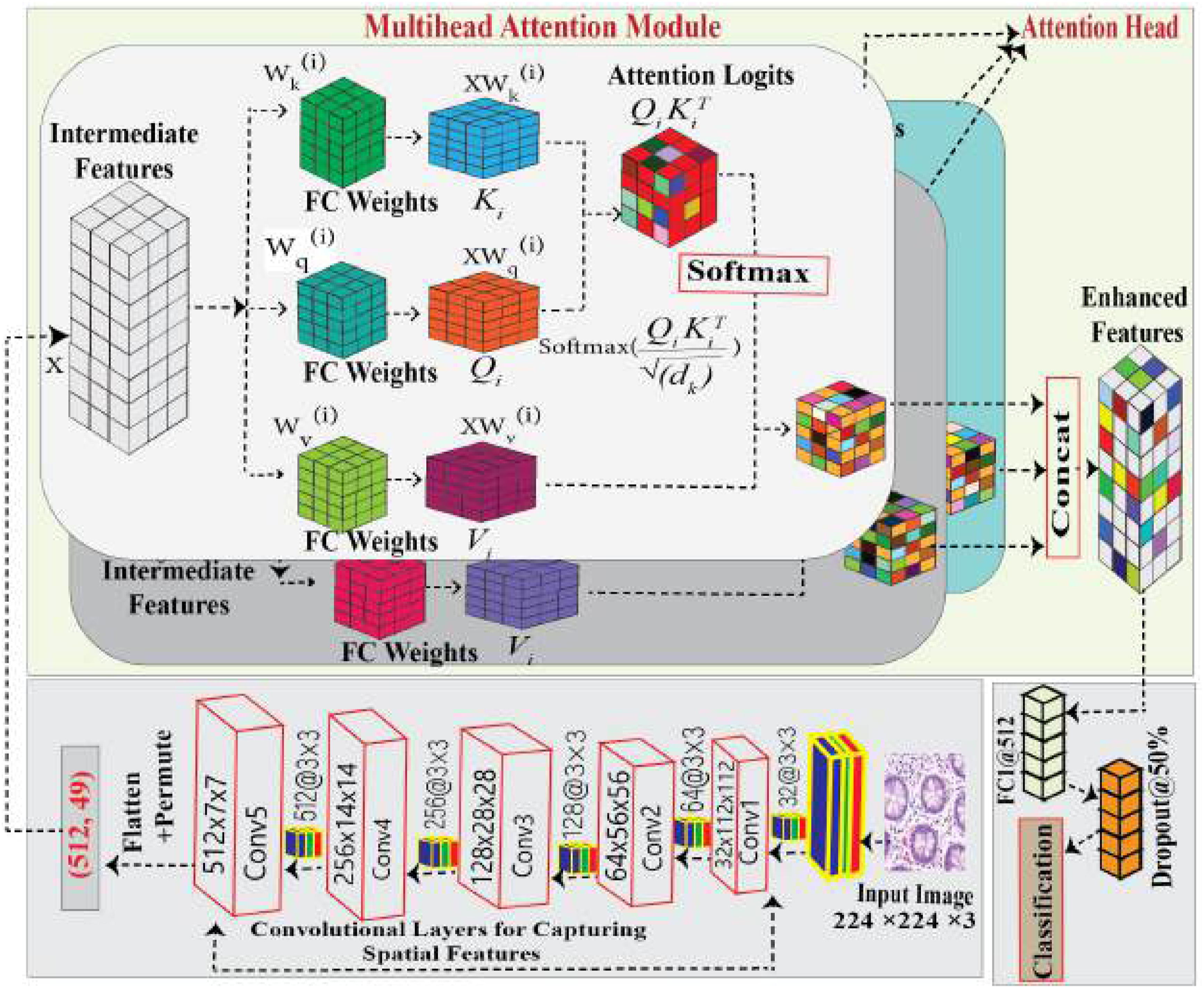
Overview of the Multi-Head Attention-Based CNN architecture for Lung and Colon Cancer Histopathology Classification.

3.4.1. Spatial feature extraction

The input images are processed sequentially through a series of layers designed to extract spatial features. This sequence comprises convolutional layers, batch normalization, ReLU activation, and max pooling, applied in blocks as illustrated in Figure 4. Each block progressively refines the spatial features, capturing essential patterns such as edges, textures, and structures. Below, we provide a detailed explanation of each component involved in the spatial feature extraction process.

Convolutional Layer: The convolutional layer is fundamental in CNN architectures, enabling feature extraction from input data through convolution operations. It utilizes learnable filters (or kernels) to detect spatial features such as edges, textures, and patterns, which serve as the foundation for hierarchical feature representation in CNNs. For a two-dimensional input feature map $\mathbf{F}\in {\mathbb{R}}^{H\times W}$ , a convolutional filter $\mathbf{K}\in {\mathbb{R}}^{k_h\times k_w}$ produces an output feature map $\mathbf{G}\in {\mathbb{R}}^{H^{\prime }\times W^{\prime }}$ as follows:

$G(u,v)=\sum _{i=1}^{k_h}\sum _{j=1}^{k_w}F(u+i-1,v+j-1)\cdot K(i,j)+b,$

(1)

where u and v represent spatial coordinates of G, initialized from 1 and incremented based on the stride s. Here, b is the bias term, and the operation involves element-wise multiplication between K and the receptive field of F. The spatial dimensions of the output are determined by:

$H^{\prime }=\frac{H+2p-k_h}{s}+1,W^{\prime }=\frac{W+2p-k_w}{s}+1,$

(2)

where p denotes padding. By applying n filters, CNNs generate n distinct feature maps, computed as:

$G_m(u,v)=\sum _{i=1}^{k_h}\sum _{j=1}^{k_w}F(u+i-1,v+j-1)\cdot K_m(i,j)+b_m,m=\mathrm{1,2},\dots ,n.$

(3)

This process enables CNNs to learn diverse features across multiple layers, making them highly effective for tasks such as image recognition and object detection.^35–37

Batch Normalization Layer: The BatchNorm2d layer serves the purpose of normalizing the output of the convolutional layer so that subsequent activation functions will have a mean value of zero and a unit variance. This helps maintain the stability and speed of the training process by limiting the internal covariate shift. For each feature channel c of a mini-batch, batch normalization is defined in the following way: Batch Normalization statically refers to the set of techniques that apply the normalization process on a neural network across a range of batch samples.

${\widehat{x}}_c=\frac{x_c-{\mu }_{\mathcal{B},c}}{\sqrt{{\sigma }_{\mathcal{B},c}^2+ϵ}},$

(4)

where,x _c is the input feature map of channel c, while ${\mu }_{\mathcal{B},c}$ and ${\sigma }_{\mathcal{B},c}^2$ are the mean and variance calculated from sub batch $\mathcal{B}$ for channel c respectively and ϵ is a constant added for numerical stability. After the normalization step, BatchNorm2d does a linear transformation to enable the network to keep the representation power of the network, and this is formulated as:

$y_c={\gamma }_c{\widehat{x}}_c+{\beta }_c,$

(5)

where γ _c and β _c are learnable parameters that scale and shift the normalized output, respectively.

Activation Function: In the design, ReLU activation function is used after batch normalization to ease training and enhance feature extraction by the model. With batch normalization, the inputs are scaled to have a mean of zero and a unit variance to avoid this saturation. Non-linearity is added by ReLU to aid the model in understanding complex structures. While some non-linearity is added by ReLU, BatchNorm prevents inputs from diverging too much. However, the amount of divergence is important because, as mentioned, positive gradients are gained from ReLU. This combination streamlines and enhances both the speed and quality of training. ReLU is defined as:

$f(x)=\max (0,x)$

(6)

ReLU activation keeps all positive values and zeros out all negative ones. It plays a role in alleviating the vanishing gradient problem, which helps improve gradient flow during training. ReLU is often used after each convolution to yield non-linear outputs. ³⁸

Pooling Layer (MaxPooling): To reduce the size of the feature maps, after each convolutional layer, MaxPooling layers are applied, which allow the network to focus on essential features. MaxPooling operation makes the computation efficient. In this operation, a small window with a fixed width and height is moved through the feature maps to extract the highest values for the window’s current position. This window will be shifted from left to right and top to bottom. At each move, the highest value among the values captured by the window on the feature map is pulled out. In this way, the data volume is reduced, enabling the model to extract relevant patterns regardless of their position.

The input feature map $\mathbf{F}\in {\mathbb{R}}^{H\times W}$ is processed by using a stride s on a window of size k _h × k _w . This results in an output feature map $\mathbf{P}\in {\mathbb{R}}^{H^{\prime }\times W^{\prime }}$ is defined as:

$P(u,v)={\max }_{i=1}^{k_h}{\max }_{j=1}^{k_w}F(us+i-1,vs+j-1),$

(7)

where u and v are the spatial coordinates of the output feature map, incremented based on the stride s. The spatial dimensions of the output feature map are computed as:

$H^{\prime }=\lfloor \frac{H-k_h}{s}\rfloor +1,W^{\prime }=\lfloor \frac{W-k_w}{s}\rfloor +1.$

(8)

assuming no padding. Pooling with overlapping windows or padding can alter these dimensions. The proposed architecture organizes convolution, batch normalization, ReLU activation, and max pooling operations into sequential blocks as mentioned earlier. Specifically, five such blocks have been applied, further refining the spatial features extracted from the input images. This block-wise design progressively enhances the hierarchical representation of features, enabling the network to capture increasingly complex patterns while maintaining robustness to variations in the input data.

After extracting spatial features through the sequential convolutional blocks, it is essential to enhance the model’s ability to capture complex dependencies and relationships within the feature maps. While convolutional layers excel at local feature extraction, they may struggle to establish long-range dependencies, critical for distinguishing subtle patterns in medical images. To address this limitation, we integrate a multi-head attention, which enables the model to selectively focus on the most relevant regions of the extracted features.

3.4.2. Multi-head attention for enhanced cancer detection

In the context of lung and colon cancer detection, accurately identifying fine-grained details within medical images is crucial for improving diagnostic performance. We incorporate the MHA mechanism after convolutional blocks in the model pipeline to address this challenge. This approach enables the network to focus on critical regions within the feature maps generated by the sequential convolutional layers, ensuring a more comprehensive understanding of the complex patterns in medical imagery. Figure 4 shows the multi-head-based proposed CNN Architecture.

Role of Multi-Head Attention in Cancer Detection: The convolutional blocks extract hierarchical features from the input images, capturing spatial and structural information. However, convolution alone may not effectively capture long-range dependencies or focus on the most relevant features for distinguishing between malignant and non-malignant regions. The MHA mechanism helps the model focus on critical areas of the feature maps. This improves its ability to detect small cancerous patterns. Figure 5 illustrates how intermediate features are processed and integrated to form enhanced features. This process leverages the attention mechanism to focus on the most informative aspects of the input, effectively refining the feature representations for improved classification performance.

Figure 5.

Architecture of the single head.

3.4.2.1. Scaled dot-product attention

The multi-head attention mechanism builds upon the scaled dot-product attention to compute relevance scores between different parts of the input feature space. Given the input feature matrix $\mathbf{X}\in {\mathbb{R}}^{T\times d}$ , where T is the sequence length and d is the input feature dimension, the mechanism first transforms the input into three separate representations:

$\mathbf{Q}=\mathbf{X}{\mathbf{W}}^Q,\mathbf{K}=\mathbf{X}{\mathbf{W}}^K,\mathbf{V}=\mathbf{X}{\mathbf{W}}^V$

(9)

Here, ${\mathbf{W}}^Q,{\mathbf{W}}^K,{\mathbf{W}}^V\in {\mathbb{R}}^{d\times d_k}$ are learnable projection matrices, and $\mathbf{Q},\mathbf{K},\mathbf{V}\in {\mathbb{R}}^{T\times d_k}$ are the resulting queries, keys, and values.

The scaled dot-product attention is computed as:

$\text{Attention}(\mathbf{Q},\mathbf{K},\mathbf{V})=\text{softmax}\left(\frac{\mathbf{Q}{\mathbf{K}}^{\top }}{\sqrt{d_k}}\right)\mathbf{V}$

(10)

The term $\mathbf{Q}{\mathbf{K}}^{\top }\in {\mathbb{R}}^{T\times T}$ represents the pairwise similarity between queries and keys. The scaling factor $\sqrt{d_k}$ helps maintain numerical stability. The softmax operation converts these scores into attention weights, and the weighted sum of V yields the final context representation $\mathbf{Z}\in {\mathbb{R}}^{T\times d_k}$ .

3.4.2.2. Multi-head attention for feature refinement

To enable the model to attend to information from different representation subspaces jointly, multiple attention heads are used in parallel. For each head j = 1, 2, …, h, separate projections are computed:

${\mathbf{Q}}_j=\mathbf{X}{\mathbf{W}}_j^Q,{\mathbf{K}}_j=\mathbf{X}{\mathbf{W}}_j^K,{\mathbf{V}}_j=\mathbf{X}{\mathbf{W}}_j^V$

(11)

where ${\mathbf{W}}_j^Q,{\mathbf{W}}_j^K,{\mathbf{W}}_j^V\in {\mathbb{R}}^{d\times d_k}$ . Each head computes its own attention output:

${\text{head}}_j=\text{Attention}({\mathbf{Q}}_j,{\mathbf{K}}_j,{\mathbf{V}}_j)$

(12)

The outputs of all heads are concatenated and projected to the final feature space:

$\text{MultiHead}(\mathbf{Q},\mathbf{K},\mathbf{V})=\text{Concat}({\text{head}}_1,\dots ,{\text{head}}_h){\mathbf{W}}^O$

(13)

where ${\mathbf{W}}^O\in {\mathbb{R}}^{(h\cdot d_k)\times d_{\text{model}}}$ is a learnable weight matrix. The multi-head mechanism enhances the model’s ability to capture diverse relationships within the input.

3.4.2.3. Feed-forward network for feature processing

Following the multi-head attention, a position-wise feed-forward network (FFN) further processes the output. It consists of two linear transformations with a non-linear activation in between:

$\text{FFN}(\mathbf{Y})=\max (0,\mathbf{Y}{\mathbf{W}}_1+{\mathbf{b}}_1){\mathbf{W}}_2+{\mathbf{b}}_2$

(14)

Here, $\mathbf{Y}\in {\mathbb{R}}^{T\times d_{\text{model}}}$ is the input, ${\mathbf{W}}_1\in {\mathbb{R}}^{d_{\text{model}}\times d_{\text{ff}}},{\mathbf{W}}_2\in {\mathbb{R}}^{d_{\text{ff}}\times d_{\text{model}}}$ , and b₁, b₂ are bias terms. The intermediate dimension d_ff expands the representation space, enabling the network to capture more complex feature interactions. The scaled dot-product attention, multi-head mechanism, and FFN form the core of the attention-enhanced representation learning in MHAB-CNN.

3.4.3. Classification steps

CNN models are composed of two sequential steps: feature extraction and classification. In the feature extraction step, a convolution operation is performed on the input image, resulting in a three-dimensional matrix or a tensor containing multiple image characteristics. In the classification step, fully connected layers, fluent with one-dimensional data, take the lead as ANN.

Flatten Layer: The Flatten layer is a crucial bridge between a CNN’s feature extraction and classification stages. It ensures that the multi-dimensional output of convolutional and pooling layers is transformed into a one-dimensional vector, making it compatible with the fully connected layers. If the output from the convolution and pooling layers is a tensor of shape (C, H, W), where C is the number of channels, H is the height, and W is the width of the feature map. Mathematically, the Flatten operator would change it to a vector of size (C × H × W). With consideration of the discussion above, this is what can be hypothesized:

$\text{Flatten}(X)=\text{reshape}(X,[C\times H\times W]),$

(15)

where X is the input tensor of volumetric size (C, H, W) and after executing Flatten operation, it produces output constructed in the form of a volume shaped into a vector (C × H × W). In this manner, the shape is created such that the next fully connected layers will treat each vector point as part of a single input feature that can be used for classification.

Dropout: The dropout layer assists in achieving better generalization for models trained using CNNs, because it can incorporate flexibility in the trained models. This is achieved by randomly turning off some input sources to the fully connected layers during training. As a result, this would enable the model to learn more complex patterns because its features are more relevant and finer. In terms of mathematics, dropout can be expressed as the following equation:

${\tilde{y}}_i=\frac{r_i{y}_i}{p},r_i\sim \text{Bernoulli}(p),$

(16)

where y _i denotes the output of the i-th neuron, where p is a parameter that defines the probability of success of sampling a neuron from the Bernoulli nucleus, and r _i is its binary rate (e.g. (p = 0.5)). During inference, dropout is not applied; rather, parameters are scaled by p to maintain the internal learned representations.

In our model, which is derived from MHAB-CNN architecture, all the fully connected layers had a dropout rate of 0.5. This approach inflicted 50% random deactivation of the neurons during the training, resulting in the network obtaining persistent and diverse feature representation. This assisted the network in learning the significant attributes within the particular classes and the general attributes that are requisite in distinguishing between the lung and colon cancer subtypes. The dropout experiments were performed deliberately, and in fact, this helped in generalization because it reduced the overfitting, which would make the model unable to perform on unseen data. In this instance, the dropout approach helped enhance the model performance against the LC25000 dataset; in this instance, increased accuracy and overfitting insensitivity were noted.

${\mathcal{L}}_{\mathit{total}}={\mathcal{L}}_{\mathit{classification}}+\lambda {\mathcal{L}}_{\mathit{dropout}},$

(17)

In this equation, ${\mathcal{L}}_{\mathit{dropout}}$ is the loss regularized due to dropout, and λ is the hyperparameter that contains the regularization term, which balances the contribution to the overall loss function. ³⁹ illustrated the efficiency of the dropout technique in a variety of neural network architectures, and it became the de facto standard for achieving excellent generalization in contemporary deep learning models.

Fully Connected Layers: A fully connected (FC) layer is a significant part of the deep learning model. Using this layer, the non-linearity of the data pattern is captured. Here, each neuron is connected with all the neurons of the previous layers. Similarly, that same neuron is connected to all the next layer’s neurons. This layout of the neurons helps to combine the features and learn patterns. The output of each neuron is calculated from the weighted sum of the inputs from the neurons from the previous layers, adding a bias to that weighted sum. After that, an activation function is applied to these intermediate results, which is written in the following equation:

${\tilde{y}}_m=g\left(\sum _{n=1}^N{\alpha }_{mn}{\tilde{x}}_n+{\beta }_m\right),$

(18)

where ${\tilde{y}}_m$ is the output of the m-th neuron, and ${\tilde{x}}_n$ is the input from the n-th neuron of the previous layer. α _mn denotes the weight, while β _m indicates the bias. The function g(⋅) is the activation function. A popular activation function is ReLU, defined as:

$g(z)=\max (0,z),$

(19)

where the convolutional layer extracts the input features, FC layers help to predict which class the input fits. The number of the FC layers depends on the dataset. However, for the classification task, the number of neurons of the last FC layer equals the number of classes used for classification. The softmax activation function is used in this previous layer to transform the input into probabilities. This operation can be defined in the following equation:

$\varphi (s_k)=\frac{\exp (s_k)}{{\sum }_{l=1}^C\exp (s_l)},$

(20)

where s _k is the input of the k-th neuron, and C is the total number of classes. This function ensures that the sum of the output will be one. Finally, the predicted class $\widehat{y}$ is selected with the class having highest softmax probability:

$\widehat{y}=\arg \underset{k}{\max }\varphi (s_k).$

(21)

This method helps the model decide which class the input belongs to.

3.5. Individual model training and validation

The experimental dataset is split into k-Folds, where k ∈ {1, 2, …, 10} and each fold has its train and validation subset. These training and testing sets from each fold have been used to train the proposed MHAB-CNN, and after that, the performance of the trained model is verified using the testing set. In this way, ten distinct models (M _k ) were created from every 10-folds where k ∈ {1, 2, …, 10}. Each of these trained models’ validation accuracy is recorded for consideration in creating an ensemble approach.

3.6. Ensemble model construction

An empirical analysis was conducted to select the top-performing models based on validation accuracy from the set of individual models {M₁, M₂, …, M₁₀}. To improve overall classification performance and robustness, these selected models were combined to form ensemble models by aggregating their predictions. The selection of models for the ensemble was guided strictly by validation performance, ensuring rigorous evaluation and avoiding data leakage from the held-out test set. In this study, two common ensemble strategies—Mean Aggregation and Voting—were applied to evaluate the effectiveness of combining multiple models in enhancing predictive performance.

3.6.1. Mean aggregation

This approach works by taking the mean probability output from the selected models. In the end, the average probability for each class is calculated, and the top class is output as the final prediction. There are two straightforward procedures:

1. Mean Probability Calculation For Each Class: For each class $c\in \mathcal{C}$ , calculate the average probability:

$P_{\text{mean},c}(x)=\frac{1}{N}\sum _{i=1}^N{P}_{M_i,c}(x),$

(22)

where N is the total number of models and $P_{M_i,c}(x)$ is the probability of model i for class c.

• 2. Class Selection Based on the Highest Mean Probability: Predict the final class label by choosing the class with the highest P_mean,c(x):

${\widehat{y}}_{\text{mean}}(x)=\arg \underset{c\in \mathcal{C}}{\max }{P}_{\text{mean},c}(x).$

(23)

This approach incorporates the subjective probabilities of each model’s output, resulting in improved outcomes. Total certainty is taken into account from all models when probabilities are averaged.

3.6.2. Voting ensemble

The final class label in this approach is obtained using an ensemble technique, known as majority voting. In the selection, each model has the power to issue a vote for the class that the model predicts, and this is done in a series of steps as follows:

1. Count the total votes for each class $c\in \mathcal{C}$ :

$V_c(x)=\sum _{i=1}^N\left[{\widehat{y}}_{M_i}(x)=c\right],$

(24)

where $\left[{\widehat{y}}_{M_i}(x)=c\right]$ equals to 1 if class c is predicted by the i-th model, else it is equal to 0.

• 2. Determine the final predicted class by selecting the class with the highest vote count:

${\widehat{y}}_{\text{vote}}(x)=\arg \underset{c\in \mathcal{C}}{\max }{V}_c(x).$

(25)

The chosen ensemble voting method is used per the consensus the models provide. The decision that is favored by the votes is selected as the outcome. Voting ensemble and mean aggregation are balancing techniques. While means aggregation offers probabilistic decisions on which prediction is most probably correct, the voting ensemble looks at the cast votes to make decisions, making it more robust to outliers or noise. Combining these methods to improve the accuracy and reliability of ensemble predictions is possible since they use different models.

3.7. Evaluation of ensembles

A test set held out from the training data is used to evaluate the constructed ensembles. This evaluation is intended to be both an objective and an accurate assessment of the performance of the ensembles constructed. The collection of measures used for assessment is exhaustive with respect to the aspects of classification effectiveness. Accuracy computes the proportion of the instances that have been correctly classified out of all the cases. In contrast, precision indicates the fraction of true positives from the tested optimistic predictions made by the model, which demonstrates the model’s accuracy. Recall or sensitivity quantifies the model correctly identifying positive instances, indicating how complete a model is in its specification. The F1-score which is defined as the average of the precision and recall may be helpful in such situations about class recognition. Cohen’s Kappa, in addition, allows for determining consensus that may occur purely by chance, even if or when the failure to reach an agreement has enabled specific measures’ results to be more complex. Together, these measures provide a good and comprehensive view of the effectiveness of the ensemble models trained in the cancer classification problem.

3.8. Visualization and robustness analysis

In verifying the interpretability and reliability of the developed ensemble models, the Grad-CAM visualizations are then used on the test samples. It uses the gradients of the output with respect to the feature maps and tries to focus on the image regions deemed necessary by the model in a given instance. Figure 12 presents representative results of Grad-CAM visualizations for the test samples of the models applying the proposed methodology, which supports the validity of the developed method.

4. Results

This section commences with a brief overview of the Environment Setup and Experimental Settings, before focusing on the Evaluation Metrics. In what follows, we provide the Numerical Results of our work. Then we turn to Grad-CAM Visualizations and Ensemble Justification. The final subsection of the section is dedicated to the Ablation Study.

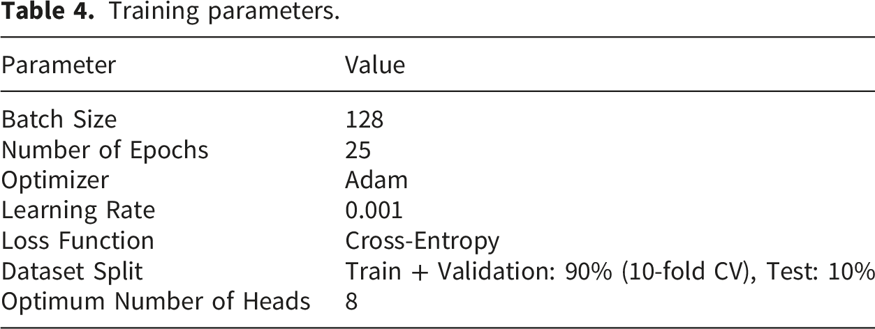
4.1. Environment Setup and experimental settings

Every experiment used a computing system with an AMD Ryzen 9 7950X 16-core CPU (2.8 GHz), 16 GB of RAM, and an NVIDIA RTX 4090 GPU (24 GB). The system runs on a 64-bit operating system, and the implementation was done using PyTorch 2.0.1 and Python 3.11.4. As illustrated in Table 4, training parameters start with cross-entropy loss with a batch size of 128, 25 training epochs, and an Adam optimizer with a learning rate of 0.001. The dataset was partitioned into 90% for training and validation (processed via 10-fold cross-validation) and 10% as an independent test set.

Table 4.

Training parameters.

Parameter	Value
Batch Size	128
Number of Epochs	25
Optimizer	Adam
Learning Rate	0.001
Loss Function	Cross-Entropy
Dataset Split	Train + Validation: 90% (10-fold CV), Test: 10%
Optimum Number of Heads	8

4.2. Evaluation matrices

In this study, we discuss how the performance of our model can be evaluated using multiple important metrics. The suite of metrics that we discuss includes accuracy, precision, recall, F1-score, Cohen’s Kappa, confusion matrix, ROC curves, accuracy curves and loss curves against epochs. Cohen’s Kappa is an index used to adjust the classification accuracy in the context of chance level agreement when comparing how predicted labels relate to actual labels. There are many instances of class imbalance, and accuracy is often misleading, and this metric is rather useful in those cases. If the class labels are not uniformly distributed, Cohen’s Kappa offers an advantage over the other metrics in that it measures how effective the model is while adjusting for the chance agreement ⁴⁰ :

$\kappa =\frac{p_o-p_e}{1-p_e},$

(26)

where p _o is the manually created contacts and p _e is the contacts created by chance.

The Receiver Operating Characteristic (ROC) curve describes the graphical representation of the relationship between the sound range output of the recall and the false error rate at different threshold levels, which have been set. The area under the curve (AUC) is a global metric indicating the overall model’s capability to discriminate, and the model is ranked with respect to AUC – the higher the AUC value, the better the model. ⁴¹ With these metrics combined, we aim to deliver a qualitative and quantitative evaluation of our model’s performance from all angles.

4.3. Numerical Results

Ten implementations of the MHAB-CNN model were trained one at a time on a selected fold of a 10-fold dataset. Each model learned the assigned fold during training for 25 epochs. Different patterns have been captured because the folds are not strictly overlapping. Ensembles have been constructed after training all ten models. Based on the validation accuracy ranking obtained during 10-fold cross-validation, models M1, M6, and M9 were selected to form the E3 ensemble. The metrics of interest are precision, loss, and ROC curves.

Models M1, M6, and M9 have been trained and validated for 25 epochs as indicated in Figure 6. The first column displays accuracy as a function of epoch, whereas the second column displays loss as a function. Figure 6(a) shows the evolution of the training and validation accuracy of model M1 versus the number of epochs. In terms of metrics, training, and validation, there is a constant enhancement throughout epoch 2. In the third epoch, there is a short drop in the validation accuracy, followed by a rise. Subsequent validations display an increasing trend but with slight oscillation, notably around the fifth epoch, where the accuracy is roughly highest. However, in all epochs, the training accuracy also advances smoothly, but with minor oscillations. The validity accuracy at the end of the final epochs shows an upward trend despite some oscillations. Figure 6(b) displays the loss curves for the training and validation datasets of model M1, which shows a similar pattern in that the losses were also reducing over time. Figure 6(c) demonstrates the accuracy curve of the model M6 and the trend of training and validation accuracy with respect to the epochs. The loss curve of model M6 is presented in Figure 6(d), which shows the trend of training and validation losses throughout the training. Similarly, M9 is illustrated in Figure 6(e) accuracy curve, whereas its loss curve is presented in Figure 6(f). In composite, these subfigures narrate the learning of the M6 and M9 models as they display the accuracy and loss measures over epochs. So, all models M1, M6, and M9 succeed in learning, as we notice training and validation accuracies getting higher and higher, while training and validation losses getting lower and lower, but these models were at times hard on the validation set.

Figure 6.

Training and validation curves for models M1, M6, and M9 over 25 epochs. The left column shows accuracy vs. epoch, while the right column shows loss vs. epoch.

Figure 7(a) and 7(b) show the ROC curves for the training and testing sets of model M1 across five classes: Co_aca, Co_n, Lu_aca, Lu_n and Lu_scc. The AUC values take on a value of 1.0 except for Lu_aca and Lu_scc in both validation and test, indicating a slightly poor separation for these classes. Models M6 and M9 show a comparable performance trend, and their training and test ROC curves are located in Figure 7(c)–7(f), respectively. Again, these models have relatively high AUC values, except for Lu_aca and Lu_scc, where slight variations are noted. In Figure 8, the mean and voting ensemble of M1, M6, and M9 models’ performances improved greatly, resulting in AUC of 1.00 across all five classes. This further demonstrates the strength of the ensemble strategy in improving classification performance, especially for difficult classes.

Figure 7.

ROC Curves for models M1, M6, and M9 on validation and test sets. The left column shows ROC curves for the validation set, while the right column shows ROC curves for the test set.

Figure 8.

ROC curve on test data of E3 (a) mean ensemble (b) voting.

Table 5 shows the performance metrics across the ten folds of the MHAB-CNN model. Each fold was assessed explicitly in terms of training accuracy, validation accuracy, precision, recall, and Cohen′s kappa, which complement each other in demonstrating how stable and efficient the model is across different dataset splits. Generally, the training accuracy was persistently above 99.82% for all the folds, with close to perfect accuracy (99.98% and above) in some folds. Validation accuracy is consistently high within the range of 99.6444% to as high as 99.9111%, regardless of the validation set used. This indicates that the model will perform well when faced with new data. Furthermore, Precision and recall across the folds, in addition to their mean, also tend to be consistent with most folds reporting 0.9991, meaning that the model classifies a good portion of positive instances with some positive misclassification. In addition, Cohen’s kappa values largely agreed with Precision, and recall values were always significantly close to or above 0.9978, showing a good level of similarity between the predicted class and the actual class.

Table 5.

Performance metrics across different folds.

Fold	Train accuracy (%)	Val accuracy (%)	Precision	Recall	Cohen kappa
1	99.9753	99.9111	0.9991	0.9991	0.9989
2	99.9703	99.8222	0.9982	0.9982	0.9978
3	99.8863	99.6444	0.9964	0.9964	0.9956
4	99.9506	99.8222	0.9982	0.9982	0.9978
5	99.9802	99.8667	0.9987	0.9987	0.9983
6	99.9802	99.9111	0.9991	0.9991	0.9989
7	100.000	99.8222	0.9982	0.9982	0.9978
8	99.9802	99.8222	0.9982	0.9982	0.9978
9	99.8269	99.9111	0.9991	0.9991	0.9989
10	99.9802	99.9111	0.9991	0.9991	0.9989

In Table 6, the independent held-out test set (10% of the LC25000 dataset) is used to evaluate ten models (M1 to M10). Each model uses nine folds for training and the remaining one fold for validation (e.g., model M1 is validated on fold 1 and trained on folds 2 to 10, model M2 is validated on fold 2 and trained on folds 1 and 3 to 10). The results indicate that the models have high accuracy and precision since most scores were greater than 0.998. This shows how effective the fold-specific training is. Models M1, M5, and M10 are the most accurate with a 0.9992 across all metrics. This suggests that the labels predicted matched the true label very well. In contrast, slightly lower scores were shown by M3 and M7, M3 being at 0.9964 and M7 being lower at 0.9924. All models achieved high Cohen’s kappa values that indicate high agreement between predictions and actual classifications. M7 achieved the lowest value at 99.05. All other models had AUC scores that are at 1.00. This suggests that the models have a great ability to differentiate between the classes. Although some individual models (e.g., M1, M5, and M10) achieved the highest test accuracy compared to validation accuracy, the model with the highest validation accuracy was considered for constructing an ensemble to avoid data leakage.

Table 6.

Performance of nine top models.

Model	Test result
	Accuracy	Precision	Recall	F1 Score	Kappa	AUC
M1	0.9992	0.9992	0.9992	0.9992	0.9990	1.0000
M2	0.9988	0.9988	0.9988	0.9988	0.9985	1.0000
M3	0.9964	0.9964	0.9964	0.9964	0.9999	0.9999
M4	0.9988	0.9988	0.9988	0.9988	0.9985	1.0000
M5	0.9992	0.9992	0.9992	0.9992	0.9990	1.0000
M6	0.9988	0.9988	0.9988	0.9988	0.9985	1.0000
M7	0.9924	0.9927	0.9924	0.9924	0.9905	1.0000
M8	0.9968	0.9968	0.9968	0.9968	0.9960	1.0000
M9	0.9980	0.9980	0.9980	0.9980	0.9975	1.0000
M10	0.9992	0.9992	0.9992	0.9992	0.9990	1.0000

Table 7 outlines the composition of four ensemble models: E3, E5, E7, and E9, which are created using individual models ranked by their validation accuracy. According to validation accuracy from higher to lower, the models are ranked in the sequence of M1, M6, M9, M10, M5, M2, M4, M7, and M8. Ensemble E3 consists of the top three performing models, M1, M6, and M9. E5 is created by extending E3 by adding models M10 and M5. Similarly, E7 is made by extending E5 by incorporating models M2 and M4. Finally, ensemble E9 is an extension of E7 by adding two more models, M7 and M8.

Table 7.

Composition of ensemble models and their constituent individual models.

Ensemble model	Constituent individual models
E3	M1, M6, M9
E5	M1, M6, M9, M10, M5
E7	M1, M6, M9, M10, M5, M2, M4
E9	M1, M6, M9, M10, M5, M2, M4, M7, M8

Table 8 presents the performance of the voting ensemble and mean ensemble for model groups E3, E5, E7, and E9. The evaluation metrics include accuracy, precision, recall, F1-score, Cohen’s kappa, and AUC. For E3, the voting ensemble obtained perfect scores in all metrics, including an AUC of 1.00. Nevertheless, the mean method also performed well, with high scores of 0.9996 for accuracy, precision, recall, and F1-score, and an AUC of 1.00. Hence, it can be observed that both methods are effective, with a slight edge for the voting method.

Table 8.

Performance of voting and mean-based ensemble approaches for different numbers of models.

Models	Ensemble type	Accuracy	Precision	Recall	F1 score	Kappa	AUC
		(%)	(%)	(%)	(%)
E3	Mean	0.9996	0.9996	0.9996	0.9996	0.9995	1.0000
	Voting	1.0000	1.0000	1.0000	1.0000	1.0000	1.000
E5	Mean	1.0000	1.0000	1.0000	1.0000	1.0000	1.0000
	Voting	0.9996	0.9996	0.9996	0.9996	0.9995	1.000
E7	Mean	0.9996	0.9996	0.9996	0.9996	0.9995	1.0000
	Voting	0.9996	0.9996	0.9996	0.9996	0.9995	1.00
E9	Mean	0.9996	0.9996	0.9996	0.9996	0.9995	1.0000
	Voting	0.9996	0.9996	0.9996	0.9996	0.9995	1.000

In group E5, all metrics reached perfect scores using the mean method. Additionally, the voting method performed strongly, with most scores centered around 0.9996. However, the mean method was more consistent for this group. The results for E7 and E9 remained stable, as most metrics returned consistently high scores. Accuracy, precision, recall, and F1-score were 0.9996, while the Cohen’s kappa value was 0.9995, and the AUC remained constant at 1.0000. Therefore, this confirms that these ensemble methods are reliable.

In conclusion, all ensemble methods performed strongly. The mean method performed best for E5, while the voting method showed a slight advantage for E3. It is also noted that all ensemble groups achieved an AUC of 1.0000, confirming the strong classification ability of these ensembles.

Table 9 lists the results of ensemble models obtained from the combination of any three of the four best-performing models (M1, M6, M9, and M10) based on their average validation accuracies. The goal is to analyze how the choice of models impacts ensemble performance. Averaging and voting methods are applied for each combination. The combination of M1, M6, and M9 achieved an average of 99.96% for all metrics using the averaging method and achieved 100% using the voting method. The M1, M9, M10 and M1, M6, M10 combinations also produced similar results for both methods. The combination of M6, M9, and M10 was found to perform comparatively worse, with results of 99.92%. Overall, the results demonstrate that ensembles formed from top-performing models yield favorable performance, with the voting method generally achieving the best results.

Table 9.

Performance Metrics of Ensemble Models (4 different combinations of M1, M6, M9, M10).

Combination	Ensemble model	Accuracy	Precision	Recall	F1-score	Kappa
M1, M6, M9	Averaging Ensemble	0.9996	0.9996	0.9996	0.9996	0.9995
	Voting Ensemble	1.0000	1.0000	1.0000	1.0000	1.0000
M1, M9, M10	Averaging Ensemble	0.9996	0.9996	0.9996	0.9996	0.9995
	Voting Ensemble	0.9996	0.9996	0.9996	0.9996	0.9995
M1, M6, M10	Averaging Ensemble	0.9996	0.9996	0.9996	0.9996	0.9995
	Voting Ensemble	0.9996	0.9996	0.9996	0.9996	0.9995
M6, M9, M10	Averaging Ensemble	0.9992	0.9992	0.9992	0.9992	0.9990
	Voting Ensemble	0.9992	0.9992	0.9992	0.9992	0.9990

Table 10 shows the comparison between E3 and S-CNN (Standard CNN). As noted, both models are ensembles from the three best performing models with the highest validation accuracy. The E3 achieves an accuracy score of 1.00 for all classes. In turn, the S-CNN has lower scores with 0.9960 for Co_aca and 0.9860 for Lu_scc. Both models have high scores of precisions, but the S-CNN has a lower precision score of Lu_aca at 0.99, whereas the E3 has 1.00 for all classes. A similar pattern is seen in E3 recall, where the E3 gives an output of 1.00 for all classes, and the S-CNN recall score for Lu_scc is 0.99. In the instance of F1 − score, the E3 stays at a perfect score of 1.00, whereas the S-CNN has slight drops to 0.99 at Lu_aca and Lu_scc. These results show that E3 is more reliable and performs better under challenging cases such as Lu_scc, compared to the S-CNN, even though both use the best-performing models.

Table 10.

Performance metrics comparison between Ensemble of MHAB-CNN and S-CNN across different classes on the Test set.

Class	Accuracy		Precision		Recall		F1-score
	MHAB-CNN	S-CNN	MHAB-CNN	S-CNN	MHAB-CNN	S-CNN	MHAB-CNN	S-CNN
Co_aca	1.00	0.9960	1.00	1.00	1.00	1.00	1.00	1.00
Co_n	1.00	1.00	1.00	1.00	1.00	1.00	1.00	1.00
Lu_aca	1.00	1.00	1.00	0.99	1.00	1.00	1.00	0.99
Lu_n	1.00	1.00	1.00	1.00	1.00	1.00	1.00	1.00
Lu_scc	1.0	0.9860	1.00	1.00	1.00	0.99	1.00	0.99

M1, M6, and M9 with their evolution ensembles E3 (means and ensembles voting) techniques have resulted in the confusion matrices shown in Figure 9. The dataset has 25,000 test samples divided into 5 classes. These classes are Co_aca, Co_n, Lu_aca, Lu_n and Lu_scc. Model M1 had only two misclassifications. One Lu_scc sample is misclassified as Lu_aca, and another Lu_aca sample was misclassified as Lu_scc. Model M6 had three misclassifications, one Lu_aca sample was misclassified as Lu_scc and two Lu_scc samples were misclassified as Lu_aca. Model M9 performed poorly and had five misclassifications where three Lu_scc samples were misclassified as Lu_aca, one Co_aca sample was misclassified as Co_n and then a Lu_scc sample was misclassified as Lu_aca. Using ensemble M3 methods using both the mean and voting techniques, all 25000 test samples were correctly classified, meaning minimal errors were present and especially none. This proves the efficiency of ensemble methods, as with the combination of individual model strengths, their accuracy is increased while errors are reduced. The results show how ensembles increase robustness and generalisation, and prove they enhance overall classification performance.

Figure 9.

Confusion matrices for models M1, M6, M9, and their ensembles.

In Figure 10, we present the number of instances per class where the ensemble mechanism successfully corrected errors compared to the worst-performing individual model among three models (M₁, M₆, and M₉). For each class, the maximum number of incorrect predictions across the individual models was used as the reference, and the number of instances where the ensemble produced the correct prediction was counted. From the results, we observe that no improvements were observed for the Co_aca and Lu_n categories, while one instance each was corrected for Co_n and Lu_scc. The most significant benefit was recorded for the Lu_aca category, where the ensemble corrected four instances compared to the worst individual model. The intrinsic characteristics of the LC25000 dataset can explain this pattern. Lung adenocarcinoma (Lu_aca) samples exhibit substantial morphological heterogeneity, including gland formation, nuclear size, and tissue architecture variations. Furthermore, Lu_aca shares visual similarities with both normal lung tissues (Lu_n) and lung squamous cell carcinoma (Lu_scc), increasing the likelihood of misclassification when relying on a single model. The ensemble mechanism leverages the diverse strengths of different models, mitigating individual weaknesses and achieving more robust predictions. As a result, ensemble learning proves particularly effective for complex and heterogeneous classes such as Lu_aca.

Figure 10.

Comparison of the number of instances per class where ensemble learning improved prediction accuracy over the worst-performing individual model.

4.4. Evaluation metrics and statistical validation of top-model ensemble

The deep learning models were assessed using 10-fold cross-validation. Based on the validation accuracy of the folds, we chose the top three models (M1, M6, and M9) to create ensemble classifiers utilizing weighted voting and Strict Majority Voting. To ensure consistency, the models were assessed on an identical testing dataset of n=2500 images.

The results from the individual models and their ensemble counterparts have been detailed in Table 11. Accuracy, Precision, Recall, and F1 Score were measured along with the 95% Confidence Intervals (CI). The ensemble models achieved flawless scores on all evaluation metrics, demonstrating robustness and an excellent ability to generalize.

Table 11.

Performance metrics with 95% confidence intervals for top models and ensembles.

Model	Accuracy	Precision	Recall	F1 score	Acc CI	Prec CI	Rec CI	F1 CI
Model1	0.9992	0.9992	0.9992	0.9992	0.9986–0.9998	0.9986–0.9998	0.9986–0.9998	0.9986–0.9998
Model6	0.9988	0.9988	0.9988	0.9988	0.9980–0.9996	0.9980–0.9996	0.9980–0.9996	0.9980–0.9996
Model9	0.9980	0.9980	0.9980	0.9980	0.9970–0.9990	0.9970–0.9990	0.9970–0.9990	0.9970–0.9990
WV	1.0000	1.0000	1.0000	1.0000	1.0000–1.0000	1.0000–1.0000	1.0000–1.0000	1.0000–1.0000
SMV	1.0000	1.0000	1.0000	1.0000	1.0000–1.0000	1.0000–1.0000	1.0000–1.0000	1.0000–1.0000

The 95% Confidence Intervals (CIs) were calculated using the normal approximation method:

$CI=\widehat{p}\pm z\sqrt{\frac{\widehat{p}(1-\widehat{p})}{n}},\text{where\hspace{0.17em}}z=1.96\text{\hspace{0.17em}for\hspace{0.17em}}95\%\text{\hspace{0.17em}CI,\hspace{0.17em}and\hspace{0.17em}}n=2500.$

(27)

For the ensemble models, all test samples were correctly classified. Therefore, the estimated proportion $\widehat{p}$ becomes 1.0. When $\widehat{p}=1.0$ , the variance term in the above formula becomes zero. As a result, the calculated confidence intervals appear as 1.0000–1.0000.

Additionally, to further examine the stability of the results, we applied bootstrap resampling with 1000 resamples. This approach estimates the variability of the evaluation metrics across different resampled datasets and provides more robust confidence interval estimates.

To determine whether the performance improvement from the ensemble models is statistically significant, we performed both the Paired T-Test and the Wilcoxon Signed-Rank Test using per-fold accuracy scores of the individual and ensemble models. The resulting p-values were:

• Paired T-Test: p = 0.0634

• Wilcoxon Signed-Rank Test: p = 0.2500

While these p-values are above the commonly used significance level of 0.05, this outcome is expected and can be explained by two main reasons. First, the statistical tests were conducted using the accuracy scores of each fold obtained from the 10-fold cross-validation process. This results in a relatively small sample size for the hypothesis test. Second, the models being compared already demonstrate very high performance. As a result, there is very little variance among their results. Therefore, the gap between the standalone models and the ensemble models becomes very small and difficult to detect. In situations like these, statistical tests may not have enough power to detect such small differences. As such, the relatively large p-values should be interpreted with respect to the limited number of folds and the closely matching performance values across the models. Despite this, the ensemble models achieved the best performance across all evaluation metrics, which again supports the effectiveness and reliability of the proposed ensemble method.

5. Discussion

The proposed MHAB-CNN ensemble outperforms even some of the most recognized models on lung cancer image classification, as shown in Table 12. With a perfect accuracy achievement of 100%, models like InceptionV3 (99.84%), S-CNN (99.80%), and Swin Transformer (99.12%), are left behind. Furthermore, the MHAB-CNN ensemble proves its high reliability in making correct predictions since it achieved a perfect score of 100% in precision, recall, F1-score, and Cohen’s Kappa. The MHAB-CNN ensemble is very effective. It is highly efficient because it utilizes only 2.89 million parameters compared to EfficientNet B4 (19.3 million), ResNet50 (25.6 million), and InceptionV3 (27.2 million). Fewer parameters still allow it to outperform the models mentioned earlier, making it perfect for systems with limited computing power. On the other hand, the CSAB-CNN voting ensemble (n = 7), which utilizes a majority voting scheme has 79.96 million parameters and achieves accuracy of 99.64%. The MHAB-CNN ensemble has perfect accuracy and uses far fewer parameters. Its Cohen’s Kappa score of 1.00 shows perfect agreement in predictions, outperforming all other models. Summarizing the information provided, the MHAB-CNN ensemble proves economical by delivering high accuracy with low computations. It also utilizes attention mechanisms and ensemble methods, which help the model remain efficient during microstaging. This makes it an excellent option for lung cancer diagnosis through medical imaging.

Table 12.

Comparison with state-of-the-art model.

Method	Year	Image	Parameters	Accuracy	Precision	Recall	F1-score	Kappa
Efficient B4	-	LC	19.3 M	97.72	97.72	97.72	97.72	97.15
Swin t	-	LC	28.3 M	99.12	99.12	99.12	99.12	98.9
Standard CNN	​	LC	14.42 M	99.80	99.80	99.80	99.80	99.75
CSAB-CNN ens×7	LC	79.96 M	99.64	99.64	99.64	99.64	99.55	​
ResNet50	-	LC	25.6 M	99.6	99.6	99.6	99.6	99.5
InceptionV3	-	LC	27.2 M	99.84	99.84	99.84	99.84	99.8
Proposed MHAB-CNN Ensemble	-	LC	3*2.89 M	100	100	100	100	100

Table 13 shows the comparison of various competitive works that classify lung cancer in terms of precision, recall, F1-score, and accuracy with our proposed work. The results show that the proposed method earns unrivaled marks, scoring perfect 100% in all evaluation measures. This highlights the method’s extreme precision, dependability, and strong performance and showcases its advancement to a notch above in terms of all healthcare technology evaluation measures. Fused-Feature + CNN ²¹ presents a remarkable accuracy of 99.64%, with measured precision landing at a perfect 100%, while its recall is only a bit lower at 99.85%. The advanced fusion model developed by Abd et al. ²³ has derived even better outcomes with their model attaining an outstanding accuracy of 99.94%, and precision, recall, and F1-score being equal to 99.84%. These results indicate that these models are highly effective but fall short of the perfect scores achieved by the proposed method. GC-attention + CNN ²² appears to be another model with great potential as it scores an impressive accuracy of 99.76%. However, it shows a bit of discrepancy in its precision measure, which lies at 99.60% and recall measure, which falls to 99.40%. In the same manner, LW-MS-CCN ²⁰ reaches 99.20% accuracy, as it demonstrates a reliable level of scoring for its measures but fails to achieve the most points from the highest performing models. The CSAB-CNN model achieves a strong accuracy of 99.64%, making use of attention mechanisms in classifying lung and colon cancer with high confidence.

Table 13.

Comparing Our Proposed Method with Previous Studies provides a detailed comparison between the outcomes achieved by our novel approach and those reported in earlier research efforts.

Methods	Year	CT	Visualization	Precision	Recall	F1-score	Acc(%)
U-Net 42	2023	L#	No	97.53	​	​	97.98
MobileNetV2 43	2024	LC*	Yes	​	​	​	99.32
Standard CNN	-	LC	Yes	99.20	99.20	99.20	99.20
CSAB-CNN 44	2024	LC	Yes	99.64	99.64	99.64	99.64
MPADL-LC3 32	2023	LC	No	98.18	98.17	98.17	99.27
Deep feature+ML-Ensemble 26	2022	LC	No	99.27	99.27	99.26	99.30
Ensemble-Approach 25	2024	LC	No	-	97	96	98
Metaheuristic-Ensemble DL 3	2024	LC	No	100	98.96	98.96	98.96
Vision Transformer 45	2023	LC	No	100	100	100	100
DL+KELM 24	2024	LC	No	96.7	95.7	97.6	98.9
LW-MS-CCN 20	2024	LC	No	99.16	99.36	99.16	99.20
Fusion Model 23	2024	LC	Yes	99.84	99.84	99.84	99.94
Fused-Feature+CNN 21	2023	LC	Yes	100	99.85	-	99.64
GC-attention+CNN 22	2023	LC	Yes	99.6	99.4	99.7	99.76
Proposed Ensemble	-	LC	Yes	100	100	100	100

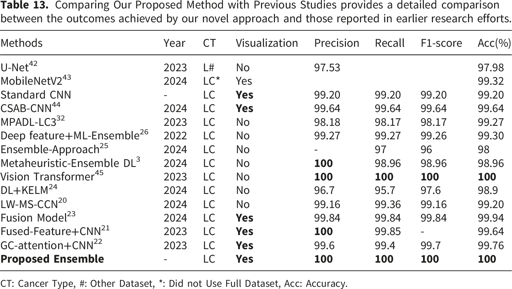
CT: Cancer Type, #: Other Dataset, *: Did not Use Full Dataset, Acc: Accuracy.

The LC25000 dataset is one of the most recognized benchmarks for the classification of histopathology images. However, past analyses of the dataset using t-SNE visualizations show that while some histopathology classes overlap and intermingle, other classes form relatively clear clusters. ⁴⁴ Such a structured distribution of features may help explain the near-perfect performance results obtained in our experiments. In future work, we plan to further assess the generalizability of the proposed MHAB-CNN ensemble by testing it on a wider range of diverse datasets that more closely resemble real-world imaging conditions.

5.1. Ablation study

As illustrated in Figure 11(a), the mean ensemble approach shows a significant improvement in performance metrics (accuracy, precision, recall, F1-score, and Cohen’s kappa) as the number of attention heads, h, is doubled, following values h = [2,4,8,16,32]. At lower values of h, particularly 2 and 4, the model achieves moderate performance, with an accuracy of 0.6376 and 0.7588, respectively. Precision, recall, F1-score, and Cohen’s kappa also show similar trends of gradual improvement. However, at h = 8, there is a sharp rise, with metrics nearing optimal values (accuracy, precision, recall, F1-score all at approximately 0.9996 and kappa at 0.9995), marking a threshold beyond which further increases in head count have negligible impact, with all metrics remaining nearly constant at their peak values. This indicates that, for the mean ensemble, h = 8 is a critical point where performance stabilizes, suggesting that further increases in computational resources for more heads may not yield significant improvements. Similarly, Figure 11(b) demonstrates the impact of increasing head count on the voting ensemble performance. At lower values of h (2 and 4), metrics are moderate, with accuracy rising from 0.6416 to 0.7508, and corresponding increases in precision, recall, F1-score, and kappa. At h = 8, all metrics reach maximum values, achieving perfect accuracy and precision of 1.0, with recall, F1 − score, and kappa similarly reaching their upper bounds. Like the mean ensemble, further increases to h = 16 and h = 32 do not contribute additional performance gains. This indicates that the voting ensemble also benefits from an increased number of heads only up to h = 8. These results suggest that while both ensemble methods benefit from a higher number of heads, particularly up to h = 8, further doubling yields diminishing returns in performance.

Figure 11.

Impact of increasing number of heads on both mean and voting E3 model.

5.2. Grad-CAM visualization and ensemble justification

To verify applicability and strengthen interpretability of the ensemble model E3, composed of M1, M6, and M9, a Grad-CAM method was used to display images that contain the regions of importance that contribute the most to the predictions made by the model. This section details how Grad-CAM was computed for each of the individual models, how the ensemble visualizations have been created, and how these have been used to support the performance of the ensemble model. Grad-CAM generates for each model Mi a class-specific localization map $L_c^{\text{Grad}-\text{CAM}}$ of interest for a class c. This is done through the use of the feature maps of a selected convolutional layer and the gradients of that feature map with respect to the output score of the class of interest. Let denote the k ^th feature map of the layer of interest as A ^k , and the score predicted for class c as y _c . The contribution of the indexed feature map k to the prediction of class c is formulated as follows ⁴⁶ :

$w_c^k=\frac{1}{Z}\sum _i\sum _j\frac{\partial y_c}{\partial A_{ij}^k},$

(28)

where Z is the spatial size of the feature map, and $\partial y_c/\partial A_{ij}^k$ is the gradient of y _c with respect to the spatial location (i, j) of A ^k . Using these weights, the Grad-CAM heatmap $L_c^{\text{Grad}-\text{CAM}}$ is computed as:

$L_c^{\text{Grad}-\text{CAM}}=\text{ReLU}\left(\sum _k{w}_c^k{A}^k\right),$

(29)

where ReLU guarantees that only the features that positively affect y _c are considered.

To facilitate the interpretation of Grad-CAM, the heat map $L_c^{\text{Grad}-\text{CAM}}$ is adjusted to the limits of zero and one and superimposed on the original image used as input. Moreover, to make the visualizations more comprehensible, two ensemble-based Grad-CAMs were created. The first visualization is the weighted average of these Grad-CAMs applied to modelsM1, M6, and M9, some or each of which predicted class c_majority, and the other Grad-CAM visualizations are based on the intersection region of each model’s Grad-CAM heatmap. The weighted average Grad-CAM for the majority-voted class c_majority is calculated as follows:

$L_{c_{\text{majority}}}^{\text{Weighted}}=\frac{{\sum }_{i\in {\mathcal{F}}_{\text{majority}}}{p}_i{L}_{c_{\text{majority}}}^{M_i}}{{\sum }_{i\in {\mathcal{F}}_{\text{majority}}}{p}_i},$

(30)

where ${\mathcal{F}}_{\text{majority}}$ denotes the set of models predicting c_majority, p _i is the confidence score of model M _i for class c_majority, and $L_{c_{\text{majority}}}^{M_i}$ is the Grad-CAM heatmap from model M _i . The intersection Grad-CAM is computed as:

$L_{c_{\text{majority}}}^{\text{Intersection}}=\underset{i\in {\mathcal{F}}_{\text{majority}}}{\min }\left(L_{c_{\text{majority}}}^{M_i}\right),$

(31)

where min is applied element-wise across the Grad-CAMs of the models in ${\mathcal{F}}_{\text{majority}}$ . Both visualizations are normalized to [0, 1] to ensure consistency and clarity when overlaid on the input image. These ensemble-based Grad-CAMs provide complementary insights: the weighted average highlights regions of consistent agreement among models weighted by their confidence. At the same time, the intersection focuses on regions unanimously important across all models, favoring the majority class. The use of ensemble-based Grad-CAMs justified the ensemble’s high accuracy (100%), even in cases where individual models made errors. By synthesizing the strengths of multiple models, the ensemble effectively captured critical features that individual models might overlook. The visualizations demonstrated that the ensemble performed robustly in classification accuracy and aligned well with domain-specific expectations of relevant image regions, thus enhancing both interpretability and trustworthiness. In Figure 12, the visualization highlights the Grad-CAM results of three selected models, M1, M6, and M9, along with their weighted average (WE) and intersection (IE) Grad-CAM heatmaps. The figure shows five vertically arranged test samples on the left, labeled (a), (b), (c), (d), and (e). For each sample, the Grad-CAM heatmaps generated by the selected models (M1, M6, and M9), as well as the WE and IE heatmaps, are shown. The prediction confidence and the corresponding Grad-CAM heatmaps for these models are examined to assess the reliability of their classifications. Among the five samples, the first three (a), (b), and (c) were misclassified by M1, M6, and M9, respectively. A red dashed rectangular box indicates the misleading regions in the Grad-CAM heatmaps for these misclassified cases. In contrast, the last two samples (d) and (e)thethreemodelscorrectlyclassify, and a black dashed rectangular box is used to highlight the common regions emphasized by the heat maps in all models. ‘The first sample, (a), belongs to the class Lung aca. Models M6 and M9 correctly classified this sample, and their Grad-CAM heatmaps highlight similar regions relevant to the classification. However, model M1 misclassified the sample as Lung scc, with its Grad-CAM heatmap deviating significantly from those of M6 and M9 by focusing on irrelevant regions. The WE heatmap is generated from Grad-CAM results of all three models, including M1, by averaging their outcomes (Grad-CAM of M1) even though M1 mispredicted the image as Lung scc. Averaging minimizes M1’s impact, allowing M6 and M9’s correct predictions to dominate. Consequently, WE heatmap now accentuates less concentrated regions corresponding to critical Lung aca features like glandular structures and mucin vacuoles, thus enhancing interpretability. In contrast, the IE heatmap displays only the focus areas common to all three models. This removes other misleading areas, including M1’s small dark region, which could indicate keratinization, more typical of Lung scc. The IE heatmap, therefore, shifts the focus to essential areas of agreement, such as those observed in glandular patterns of Lung aca. This approach is more reliable as these claimed features are checked against clinical data and are likely to be valid. This pattern is also observed in samples (b) and (c), where the misclassifications by models M6 and M9 are similarly marked by the red dashed boxes around misleading regions.

Figure 12.

Visualization of Grad-CAM heatmaps for selected models and ensemble techniques.

Throughout the remaining samples, models that agree on the same predicted class (via voting) consistently highlight similar regions in their Grad-CAM heatmaps. The WE heatmap represents the averaged relevant regions emphasized by models that voted for the same class. In contrast, the IE heatmap focuses on the intersection of these regions, showcasing only the most consistent features. These heatmaps provide a valuable tool for quick and reliable pathological analysis by highlighting averaged and common areas critical for classification decisions.

5.3. Deployment feasibility

The three metrics of parameter size, FLOPs, and inference time of the models are shown in Table 14. Each experiment was done three times, and the last column indicates the time to process 2500 test images. For the MHAB-CNN model, the three runs take 284, 339, and 308 ms time, and the average is around 310 ms (0.12 ms per image). This model is easy to deploy, as it has 2.89M parameters and 1.02 GFLOPs. Thus, it is lightweight. The ensemble model shows times of 718, 503, and 683 ms for the three runs, which averages to 635 ms (0.25 ms per image). This model, albeit slower, performs of higher value, and thus, maintains the average time taken.

Table 14.

Inference time.

Model name	Parameter size	FLOPs	Time taken (ms)/sample
MHAB-CNN	2.89 M	1.028521472 GFLOPs	284/2500, 339/2500, 308/2500
Ensemble of MHAB-CNN	3*2.89 M	3*1.028521472 GFLOPs	718/2500,503/2500, 683/2500

Overall, both models show efficiency. Nevertheless, the ensemble model exhibited improved accuracy and only suffered a small increase of time taken for inference.

6. Conclusion

In conclusion, our research demonstrates the effectiveness of MHA-based CNNs combined with ensemble learning for classifying lung and colon tissues, including benign and cancerous types. By utilizing advanced attention mechanisms and ensemble techniques, we achieved perfect performance metrics across all folds on the LC25000 dataset, including a train accuracy, validation accuracy, precision, recall, and kappa score of 100%. Grad-CAM visualizations further supported the model’s reliability by highlighting relevant regions for classification; however, formal validation of these visual explanations by expert pathologists remains an important direction for future work. These results signify a meaningful advancement in automated histopathological analysis, offering valuable insights for clinical diagnosis and treatment planning. Despite these achievements, challenges remain. The availability of diverse and comprehensive datasets is crucial for improving the model’s generalizability to a broader range of pathological conditions. Additionally, while Grad-CAM aids interpretability, further integration of explainable AI techniques is necessary to enhance trust in AI-based diagnostic tools. Future efforts could also focus on integrating the model with multi-modal datasets, including genetic or radiological data, to improve diagnostic accuracy. Other promising directions are exploring lightweight versions of the model for deployment in resource-constrained settings and incorporating continual learning mechanisms to adapt to evolving data. These advancements could bridge the gap between research and practical clinical applications, enhancing patient outcomes.