
Abstract
This article describes a methodology to recognize emotional states through an electroencephalography signals analysis, developed with the premise of reducing the computational burden that is associated with it, implementing a strategy that reduces the amount of data that must be processed by establishing a relationship between electrodes and Brodmann regions, so as to discard electrodes that do not provide relevant information to the identification process. Also some design suggestions to carry out a pattern recognition process by low computational complexity neural networks and support vector machines are presented, which obtain up to a 90.2% mean recognition rate.
Keywords
Introduction
The recognition of emotional states through a computer has been a widely studied topic in affective computing, since Rosalind W Picard proposed the basis to analyze the physiological responses of an emotion; 1 however, most of these studies have been focused on analyzing the peripheral reactions produced by emotions, such as vocal or facial expression, and some researchers suggest that these responses could be manipulated by common users and they suggest the implementation of bio-medical signals as more reliable data sources, according to the William James theory: 2 emotional states could produce disturbances in one or more of the basic human functions, such as changes in heart rate, muscle responses or temperature changes, when a person is facing a real or an imaginary emotional stimulus. There are many bio-medical signals that could be evaluated to recognize emotional states, such as heart rate or body temperature variations; however, our interest is focused on the analysis of signals that were originated by brain activity, particularly electroencephalography (EEG) due to the fact that this technique does not require extensive technical knowledge to implement and implementation costs are relatively low.
Related work
Some of the most outstanding work in emotion recognition by an EEG signals analysis, was presented by Dr M Murugappan of Perlis University in Malaysia and by Dr Sander Koelstra at Queen Mary University of London in the UK. Dr Murugappan proposed a mathematical model to infer emotional states from EEG analysis and Dr Koelstra developed the DEAP database, which is an extensive collection of physiological signal records of emotional stimulation processes, and both works demonstrates the feasibility of the establishment of a relationship between the electrical activity in brain cortex and emotional states.3 –5 A summary of related work is presented in Table 1.
Related work in classification and identification techniques of emotional states and associated identification rate (IR).
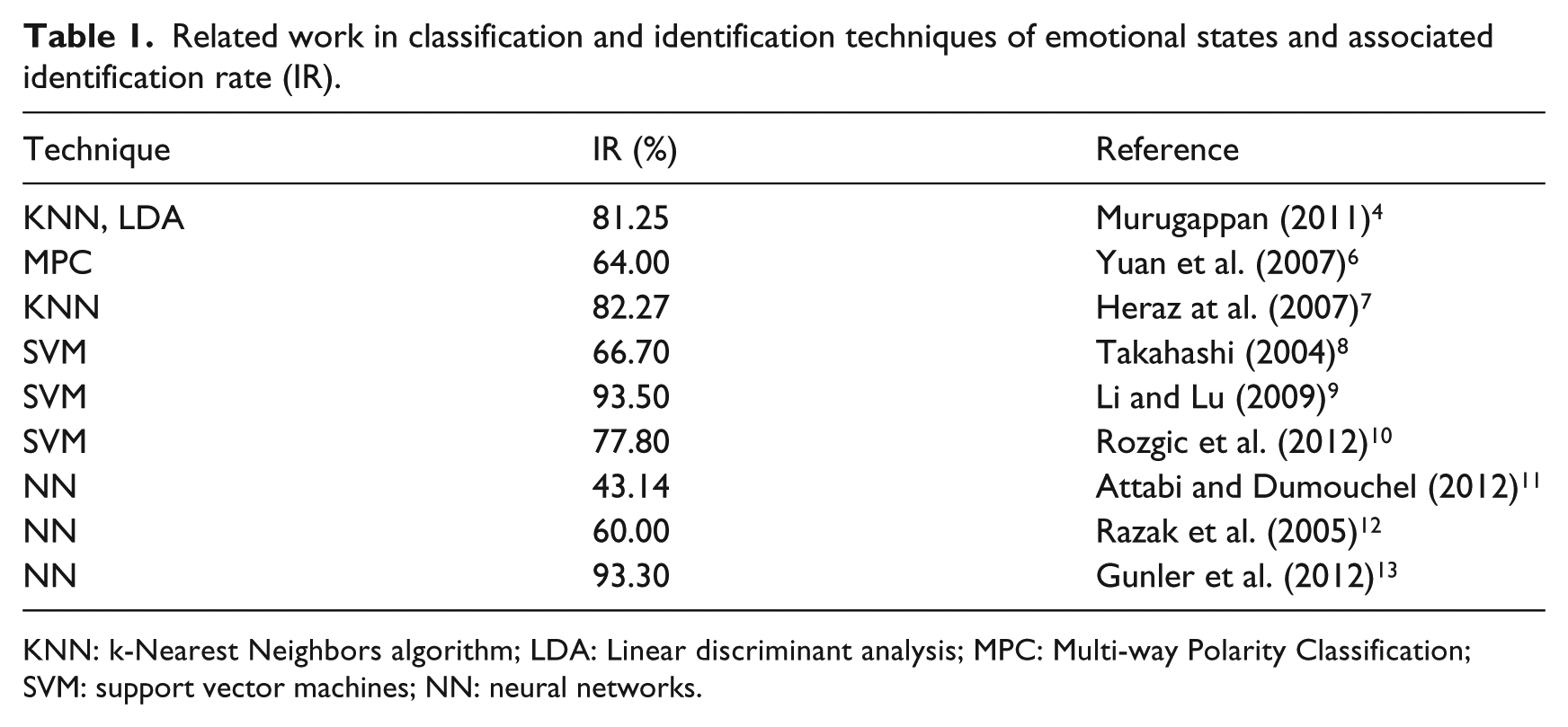
KNN: k-Nearest Neighbors algorithm; LDA: Linear discriminant analysis; MPC: Multi-way Polarity Classification; SVM: support vector machines; NN: neural networks.
Emotions
Disambiguation
Words such as affect, feeling and emotion are commonly used synonymously; however, each of them has a very different meaning, in their etymology and in the physical and mental reactions they cause.14 -16
Emotions are the manifested reactions to those affective conditions that due to their intensity, move us to some kind of action with slight or intense, concomitant or subsequent, repercussions upon several organs, that can set up partial or total blocking of logical reasoning.
Affect could be defined as a grouping of psychic phenomena manifesting under the form of emotions, feelings or passions, always followed by impressions of pleasure or pain, satisfaction or discontentment, like, dislike, joy or sorrow.17, ii
Feelings are seen as affective states with a longer duration, causing less intensive experiences, with fewer repercussions upon organic functions and lesser interference on reasoning and behavior. iii
Emotion theories
Over centuries, philosophers, physicians and psychologists have studied affectivity phenomena by questioning their origin, their role upon psychic life, their action with regards to favoring or hindering adaptation and their neuro-physiological concomitants; 18 however as established by Scherer (Scherer (2005)) “even the simple question, of what emotions are?, hardly get the same answer”. 19
There are classical and antagonistic theories of emotions:
Classical theories are supported by the Darwinian theory of emotions, which states that affective reactions are innate patterns designed to orient behavior and promote adaptation,18,20,21 and by recent theories which suggest that emotions are complex phenomena initiated by a central process as result of internal or external causes, that can be observed as an organismic alteration.19,22 -29
Antagonistic theories are led by the Claparede theory, 14 that defines emotions as useless, non-adaptive and harmful phenomena, since according to this theory emotions are characterized by a sudden disruption of an affective balance (mostly for short episodes), with slight or intense, concomitant or subsequent, repercussions upon several organs, that can set up partial or total blocking of logical reasoning in the affected subject.
It is the definition provided by Scherer (Scherer (2005)), which best fits an engineering task, defining an emotion as: an episode of interrelated and synchronized changes in most of the organismic subsystems(note call 4 and 5), in response to the evaluation of an external or internal stimulus event.
Data sources
The lack of a standardized database is one of the main problems with carrying out a study about the physiological responses of an emotional state, since standardized databases such as the International Affective Picture System (IAPS) or the International Affective Digitized Sound system (IADS) can be only implemented to perform the stimuli processes, which implies that if two different research groups perform an experimental setup that associates the same stimulus and even the same participants, the results will vary due the environmental conditions.30,31
However, there are some data collections such as bu-3DFE, PhysioNet, DEAP and the Ibug project that can help with this problem.
bu-3DFE is a collection of several physiological signal records, associated with a wide range of emotional expressions. 32
PhysioNet is a collection of physiological signals, time series and images, constructed to perform a behavior analysis. 33
The Ibug project is a collection of bio-metric data associated with affective behaviors. 34
DEAP (Database for Emotion Analysis using Physiological Signals) is a wide collection of biosignals generated by several specialized experimental setups under arousal and valence stimuli. 5
Database for emotion analysis using physiological signals
is a large collection of physiological signals which are directly associated to an emotional stimulus in a multi-modal dataset for the analysis of human affective states, where the EEG and other peripheral physiological signals of 32 participants were recorded as each watched 40 one-minute long excerpts of music videos. Participants also rated each video in terms of the levels of arousal, valence, like/dislike, dominance and familiarity they experienced. 5
This is the database that we implemented for the experimental process presented in this paper, because it is to our best knowledge the most comprehensive and reliable source of data.
Data bounding methodology
This work proposes a methodology that reduces the amount of the processed data, by defining a model that establishes a correlation criteria between emotional activity and it responses in the brain cortex and excludes regions that could not provide significant performance to the recognition process.
The Brodmann regions
Dr Korbinian Brodmann sub-divided the brain cortex into regions that appeared to have micro-structural differences and associated these regions with specific cognitive functions, such as motor processing, speech, hearing or sight. Since our work is focused on analyzing an emotional process evoked by audio-visual stimuli, we are proposing that only the electrodes that are strongly related to the audition, visual, sensory and motor vi regions vii should be considered for the digital signal processing task (see Table 2).18,35 –40
Regions of the cortex with its associations with the cerebral cortex and its relationship with Brodmann regions.
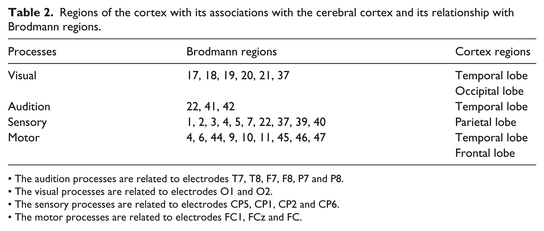
• The audition processes are related to electrodes T7, T8, F7, F8, P7 and P8.
• The visual processes are related to electrodes O1 and O2.
• The sensory processes are related to electrodes CP5, CP1, CP2 and CP6.
• The motor processes are related to electrodes FC1, FCz and FC.
Selected electrodes
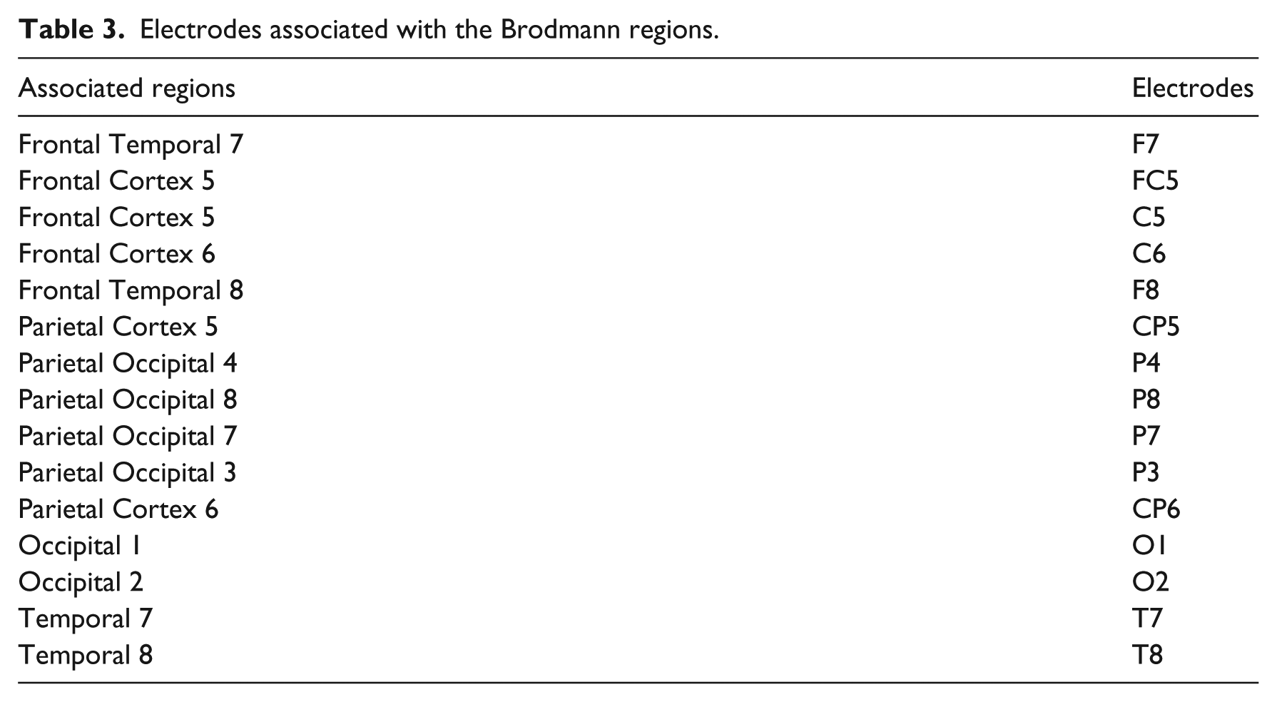
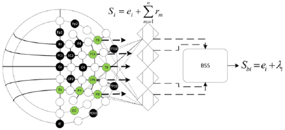
Only 15 electrodes were set as active elements, while 22 were setted as non active elements as can be observed in Figure 1 and Table 3. This provides a data reduction of 11,264 samples per second (considering a nominal sampling rate of 512 Hz), which is a significant data reduction and consequently also a computational burden reduction. viii
Electrodes associated with the Brodmann regions.
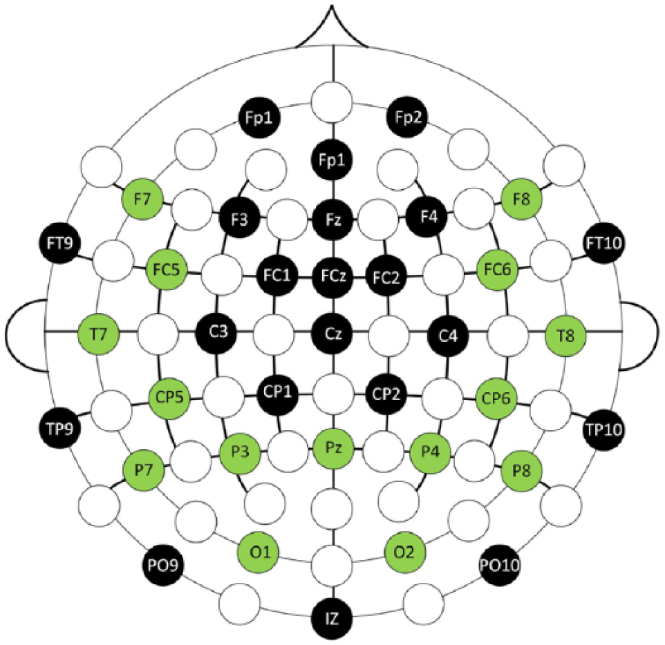
Graphical representation of the active and non-active electrodes (green electrodes are considered as active electrodes and black marked as non-active electrodes).
Signal conditioning
A very wide variety of phenomena could affect the performance of the analysis of physiological data, such as a wide variety of noise, or the large amount of resources required to process these types of signals.
Noise filtering
The Laplacian filter described by Murugappan (equation (1)), was implemented to mitigate the problem that EEG signals are naturally contaminated with noise and artifacts (i.e. eye movement(EOG), muscular movement (EMG), vascular movements (ECG) and kinetic artifacts) 4

where
Signal bounding
A band-pass filter with cutoff frequencies of 0.5 Hz to 47 Hz, was implemented to exclude all frequencies that are not associated with the brain rhythms model: delta (0.2 to 3.5 Hz), theta (3.5 to 7.5 Hz), alpha (7.5 to 13 Hz), beta (13 to 28 Hz) and gamma (
Blind source separation
A blind source separation (BSS) algorithm was implemented to remove redundancy between active elements but preserve information of non-active elements. Since these cases are generally considered as a multi-channeling problem and the signal
where
Process model of the blind source separation by independent component analysis implemented.
Feature extraction
A common question about the implementation of the wavelet transformation is ‘Why does it not use Fourier traditional methods?’. The answer is that there are two important differences between Fourier and wavelet analysis.
The first is that due to the Fourier basis, functions are localized in frequency but not in time (a small frequency change in the Fourier transform could produce changes in all parts in the time domain), unlike the wavelet transform which presents resolutions in frequency (through expansion) and in time (through translations).
The second is that many kinds of functions that can be represented by wavelets in a more compact form (i.e. functions with discontinuities and features with sharp spikes usually need fewer functions when they are analyzed on a methodology based on wavelets) and due to this, large data sets can be easily and quickly transformed by the discrete wavelet transform (the counterpart of the discrete Fourier transform) by encoding the data as wavelet coefficients, which implies a higher processing speed since the computational complexity of the fast Fourier transform is
Feature selection
Each level of the discrete wavelet transform is calculated by passing the signal through a series of filters; samples are passed through a low pass filter
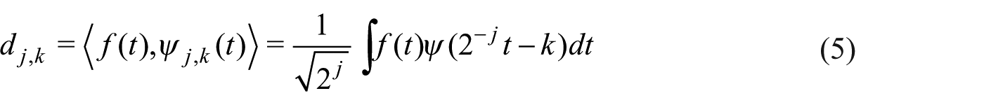
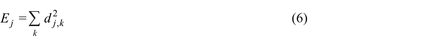
Also the energy content in a specified region of the signal
where
This same procedure can be implemented to extract the approximation coefficients.
The total coefficients energy can be expressed as
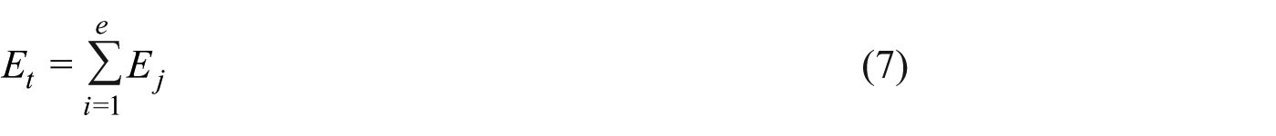
where
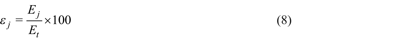
The translation and dilation coefficients, can be implemented directly as the features in the classification problem.
Classes
Our proposal to establish an appropriate model that establishes a clear distance between each emotional tag, is the assignment of a distance parameter between the emotional tags according to the Ekman, Russell and Scherer models. Since the Ekman model provides the basic tags to identify each class, while the Russell and Sceherer models define emotional states as arousal and valence levels.
This model can be observed in Figure 3, which encompasses all similar emotional states according to their arousal and valence levels (i.e. all emotions that have high levels of arousal and high levels of valence are correlated to states of happiness, states which have a low valence and high arousal are correlate to anger, low arousal and low valence to sadness, and low arousal and high valence to relaxation states).
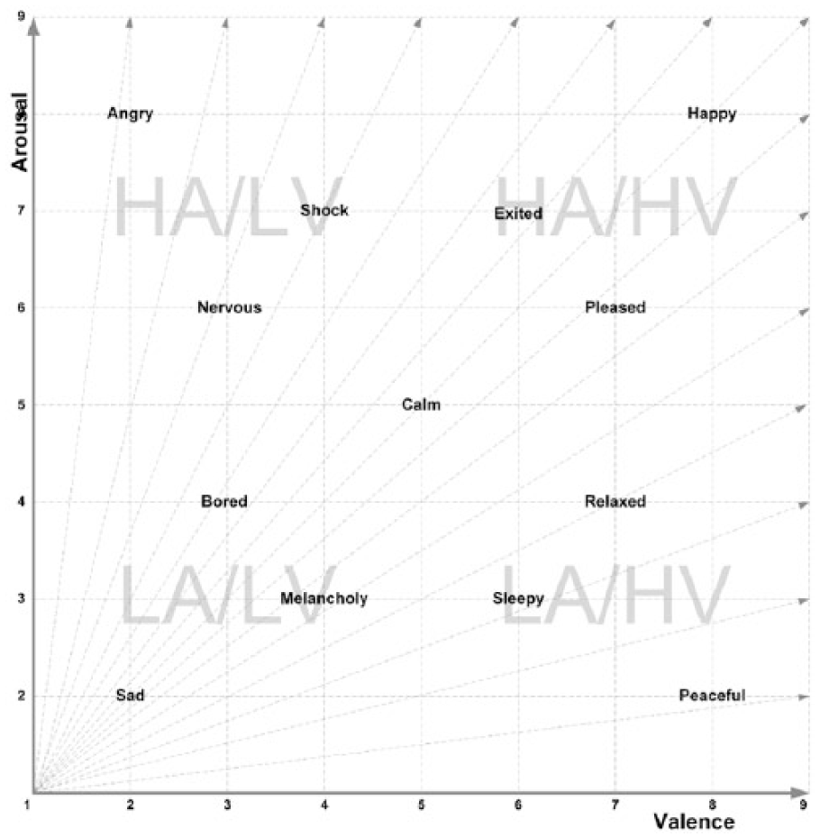
Emotional states distribution model, based on arousal and valence levels and the discrete tags of the Ekman model.
Class 1: (HA-HV) high arousal, high valence.
Class 2: (HA-LV) high arousal, low valence.
Class 3: (LA-HV) low arousal, high valence.
Class 4: (LA-LV) low arousal, low valence.
Also this model defines the orientation of each of the evoked potentials according to their characteristics to define the elements of each of the classes that would be implemented as references in the identification model, as can be observed in Figures 4 and 5, where each element of the experimental process belongs to a particular class.
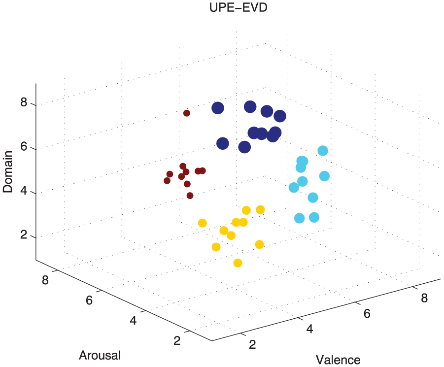
The location of the experimental cases, according to their emotional stimuli responses obtained by the user ratings (the input elements to the classification process are created based on this information). Arousal: it includes features that define idle or alert states (i.e. disinterested, boring, alert, excited). Valence: ranges from unpleasant (i.e. sad, stressed) and nice (i.e. happy, euphoric). Domination: ranging from a feeling of helplessness and weak (uncontrolled) to one feeling empowered (in control of everything).
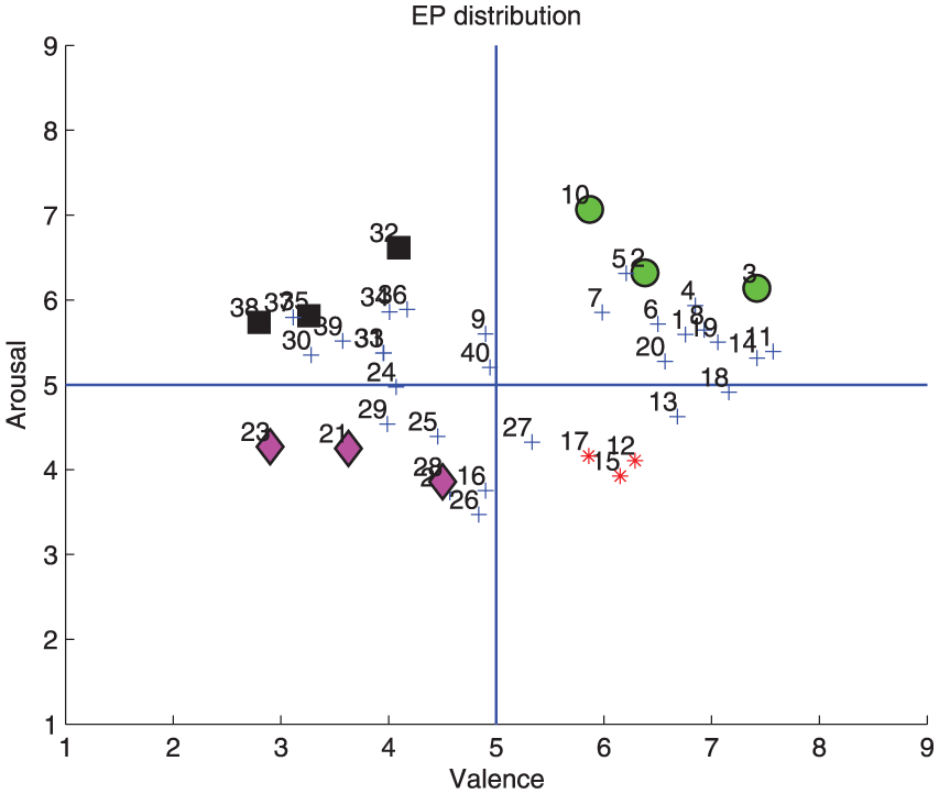
Distribution of evoked potential trials in an arousal and valence space. As seen there are ten experiments related to each class and a greater emphasis are given to three of them in relation to its distance to the other cases to ensure a greater separability between classes, according to their labeling.
Identification process
Support vector machines and neural networks, are the techniques that according to literature review have shown the best recognition rates (Table 1). Therefore, these two techniques were implemented in this work in order to corroborate the performance of our methodology.
Experimental setup and inputs
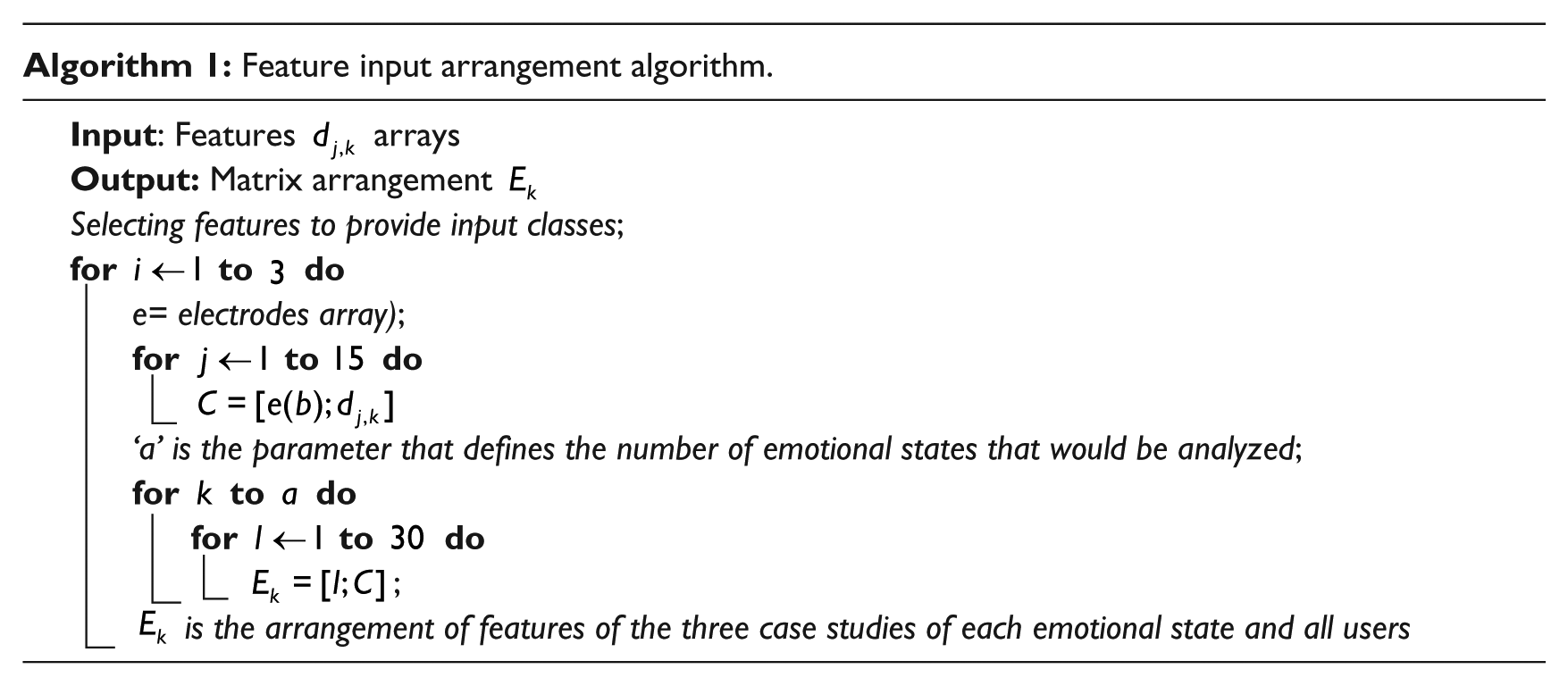
The experimental configuration presented in Figure 6, was designed to evaluate the identification performance of each of the combinations produced by implementing the clustering Algorithm 8.1, which ensures a consistent experimental process distribution for each of the elements of the classes by considering at least one experimental class associated with each class (i.e. each of the cross validations evaluate distinct cases of the same class). xi
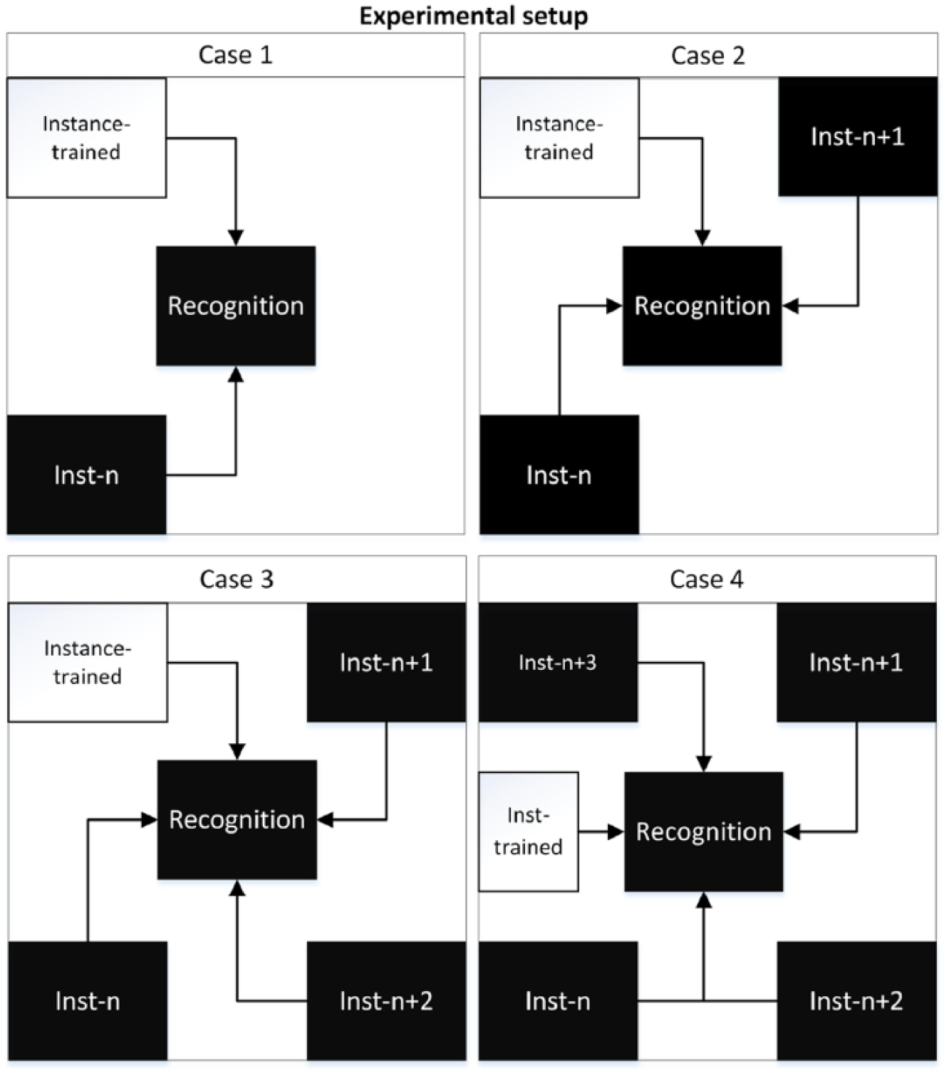
Class selection model to perform the identification performance task.
8.1.1 Classification inputs
To ensure that each case study contains the information from more than one user at the same time and to corroborate the existence of a correlation between different study subjects, each case is also assessed by means of the following classification scheme:
a: Contains the information of a single user.
b: Contains information of two users.
c: Contains information of three users.
d: Contains information for all users.
Neural networks
Artificial neural networks (NN) are computational techniques that can be trained to find solutions, recognize patterns, classify data or forecast events by defining the way its individual computing elements are connected, which automatically adjusts their configurations to solve specific problems according to a specified learning rule. Due to the fact that EEG data are considered as chaotic signals, many researchers have proposed the implementation of NN, as one of the most appropriate tools to carry out the analysis, since NN have a remarkable ability to derive meaning from complicated or imprecise data. Besides NN are inspired by the natural behavior of a neuron, and EEG signals are signals produced by neurons.
Implementation
The implementation of a highly complex NN was our initial proposal to carry out the pattern recognition task; however, as can be observed in Figure 7, the error rates have a direct correlation to the network architecture (i.e. if network architecture increases, so to does the error), contrary to our initial thought and that the implementation of low complexity architecture will be the best option for this particular case, as shown in Figure 8, where a 10-fold cross-validation was performed to evaluate 20 configurations of low complexity networks, in order to determine the amount of units per layer that would be necessary to obtain the most accurate and stable recognition rate.
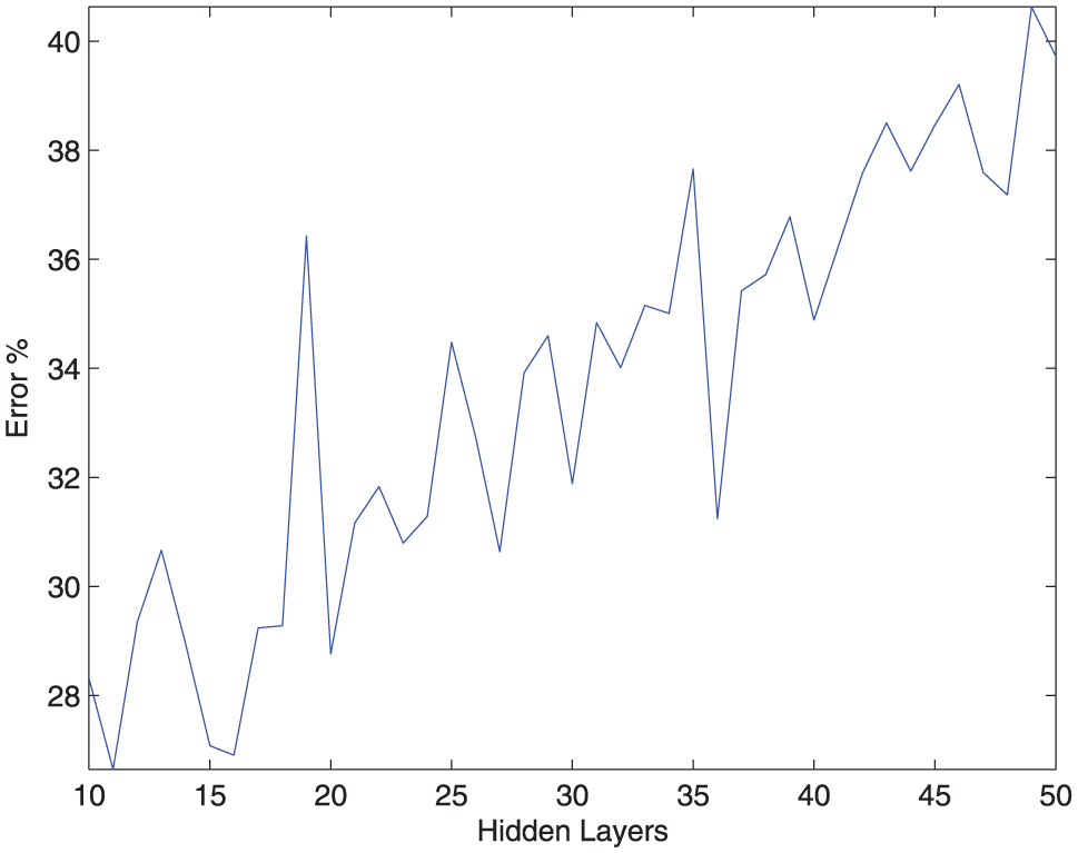
An identification process performed by the same NN configuration, but incrementing by one the number of layers in each iteration up to 50.
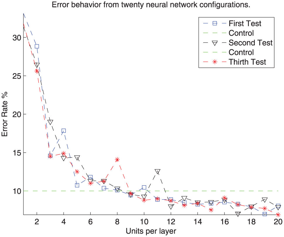
Performance of low complexity NN configurations. Considering only NN with less than 20 hidden layers, the validation process chose the number of units per layer this network would have by considering that 20 would be the maximum number of elements per layer.
Based on the presented considerations, the following NN was implemented to perform the presented experimental results: xii
resilient back-propagation algorithm;
11-layer topology, 2/3/4 units in the input layer, 18 hidden units per layer and 2/3/4 units on the output;
200 maximum epoch;
maximum square error (MSE), Goal =
70% for training data;
15% to validate;
15% to test.
Support vector machines
Support vector machines (SVM) provide separability to non-linear regions by implementing kernel functions that avoid the local minimum issues by implementing quadratic optimization, so that, unlike NN, this technique is more related to an optimization algorithm rather than to a greedy search algorithm. Also when the classification problems do not present a simple separating criterion, there are several mathematical approaches that could be applied to the SVM strategy, in order to retain all the simplicity of hyperplane separation.
Implementation
Three transformation kernels were implemented to perform the SVM identification processes:
Gaussian or radial basis
polynomial
multi-layer perceptron
Besides the fact that the training algorithm function implements an optimization method to identify vectors
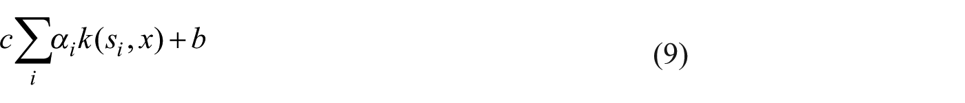
where
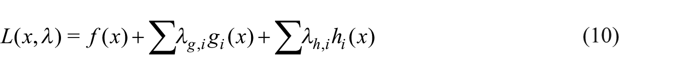
where
Results
Separability
The first thing that may be noticed is that this methodology provides a significant reduction of the computational complexity, since, as can be observed in Figures 9 to 17, the degree of separability obtained by implementing it can be easily observed and some of the behavioral tendencies can be noticed without a computational identification process.
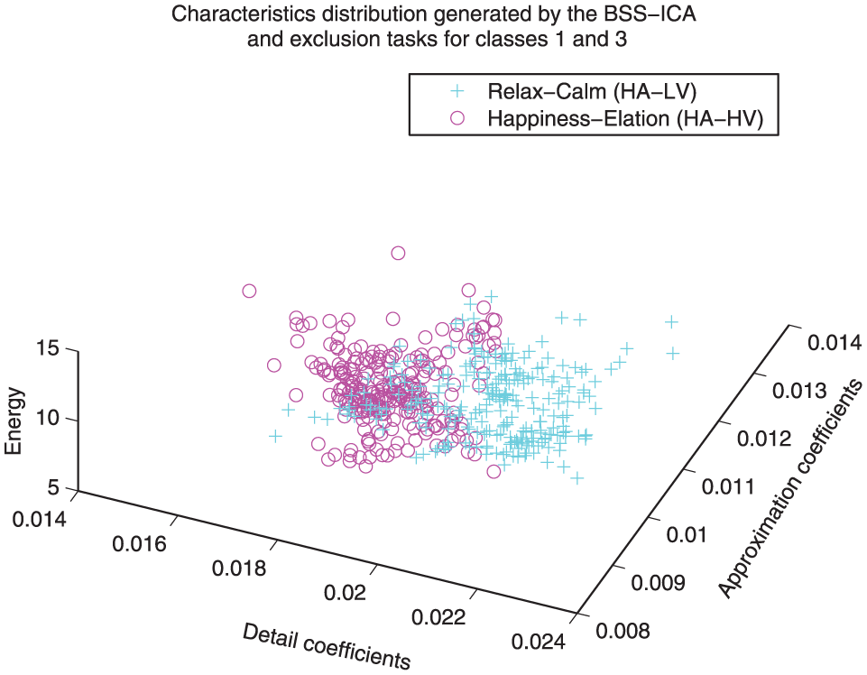
Distribution comparison between classes 3 and 1. A separation between the coefficients associated with these classes can be easily observed, even before the classification and recognition processes (class 3: relaxation/calm, class 1: happiness/elation).
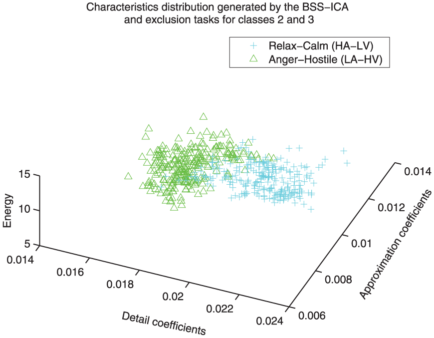
Distribution comparison between classes 3 and 2. A very clear separation between the coefficients associated with these classes can be easily observed, even before the classification and recognition processes (class 3: relaxation/calm, class 2: anger/hostile).
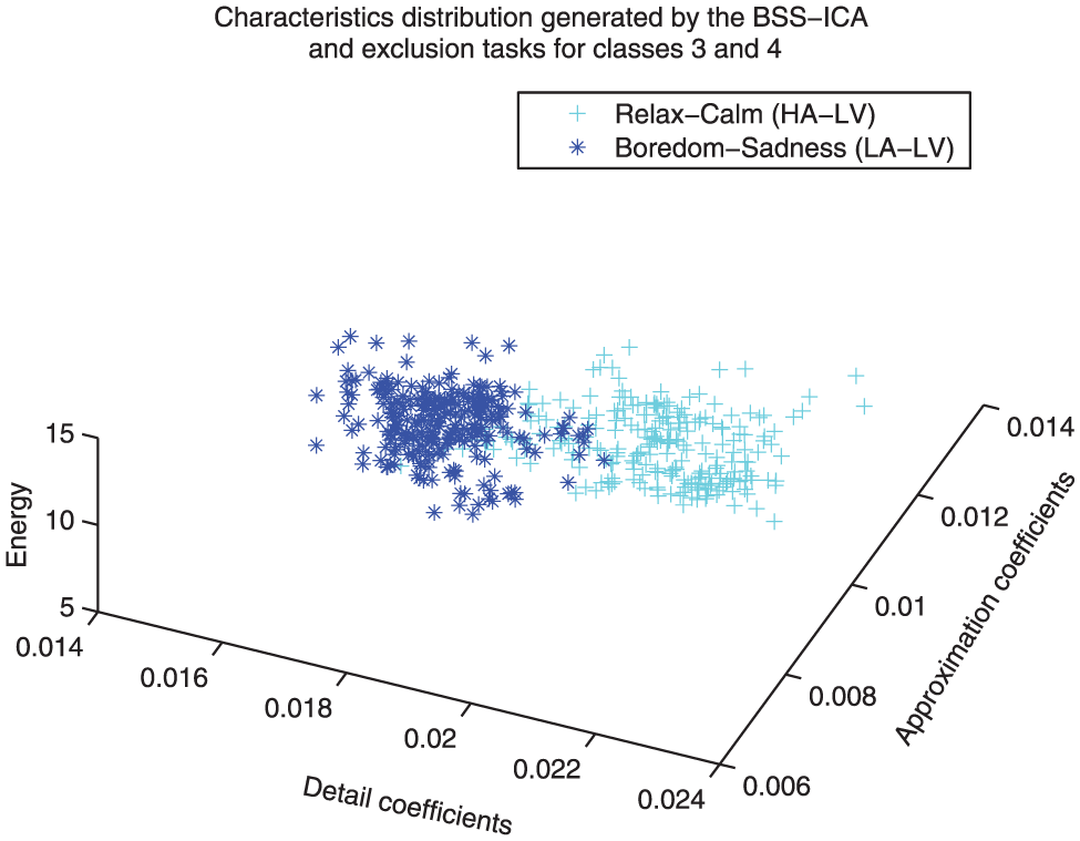
Distribution comparison between classes 3 and 4. A clear separation between the coefficients associated with these classes can be easily appreciated, even before the classification and recognition processes (class 3: relaxation/calm, class 4: boredom/sadness).
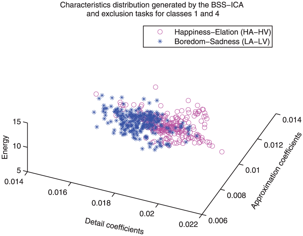
Distribution comparison between classes 1 and 4. For this case the separation between classes is not as clear as the three previous cases; however, that the separation process can be carried out with simple classification techniques can still be observed (class 1: happiness/elation, class 4: boredom/sadness).
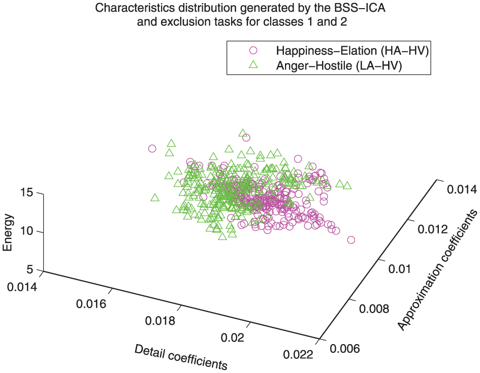
Distribution comparison between classes 1 and 2. For this case the separation between classes is not as clear as the three previous cases; however, that the separation process can be carried out with simple classification techniques can still be observed (class 1: happiness/elation, class 4: anger/hostile).
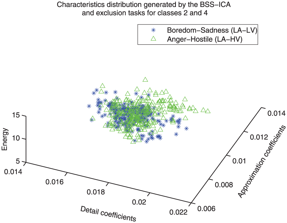
Distribution comparison between classes 4 and 2. For this case the relationship between the classes is considered very close, which could indicate very similar behavior in both classes (class 1: boredom/sadness, class 4: anger/hostile).
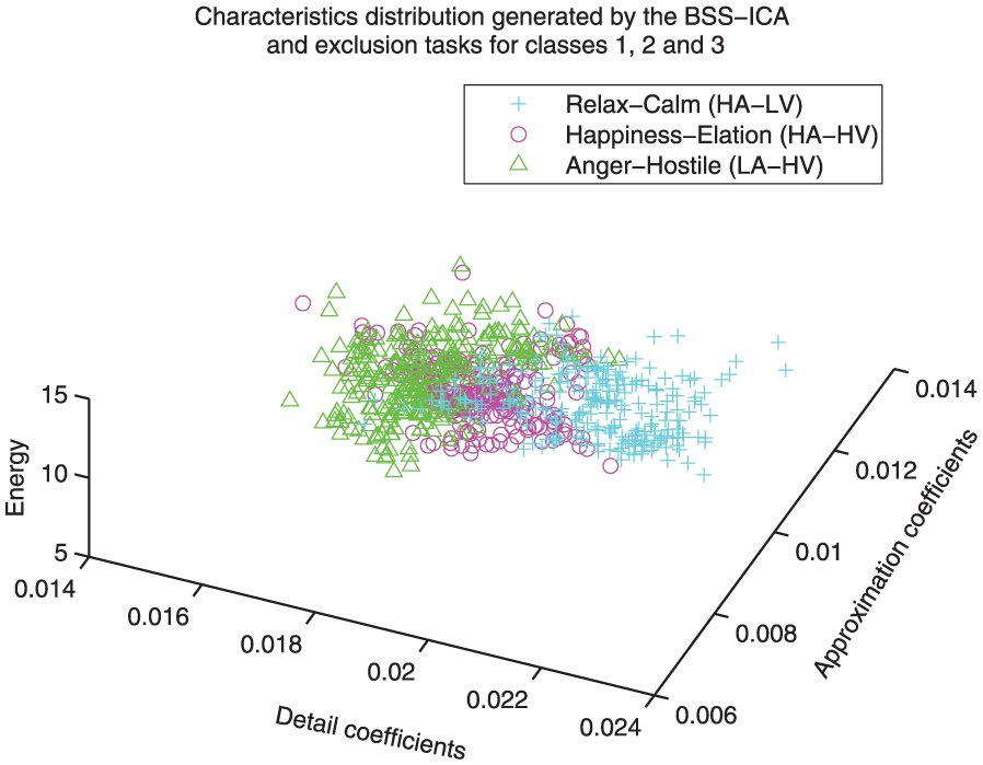
Distribution comparison between classes 1, 2 and 3. This representation shows the level of complexity for the three-class identification process (class 1: happiness/elation, class 2: anger/hostile, class 3: relaxation/calm).
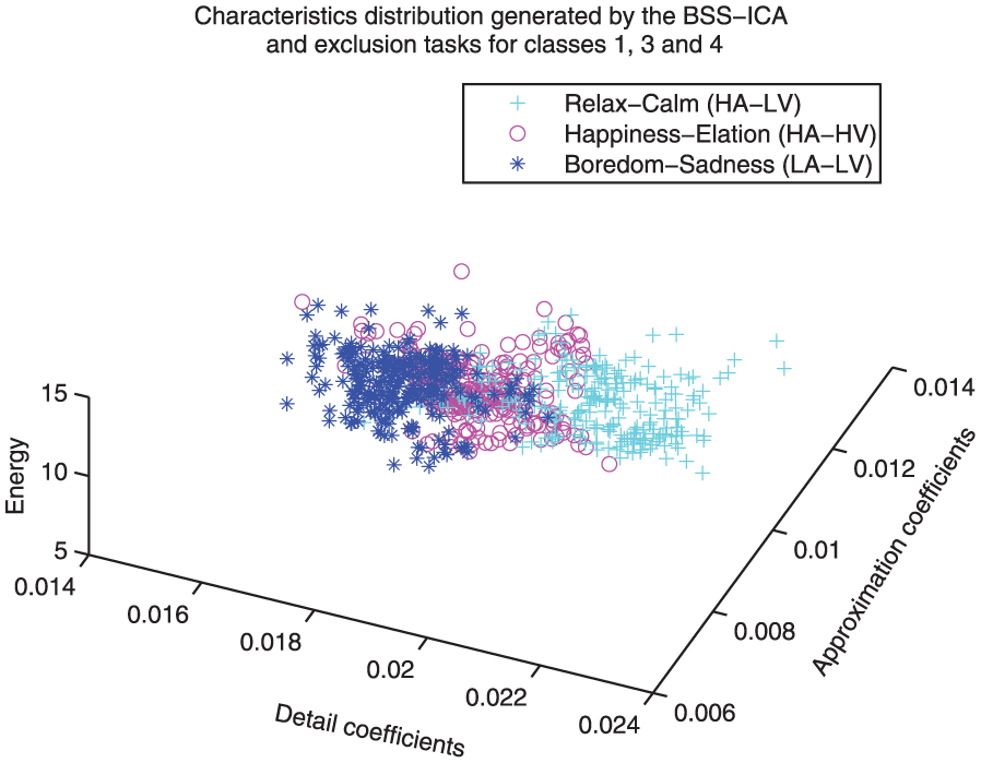
Distribution comparison between classes 1, 3 and 4. This representation shows the level of complexity for the three-class identification process (class 1: happiness/elation, class 3: relaxation/calm, class 4: boredom/sadness).
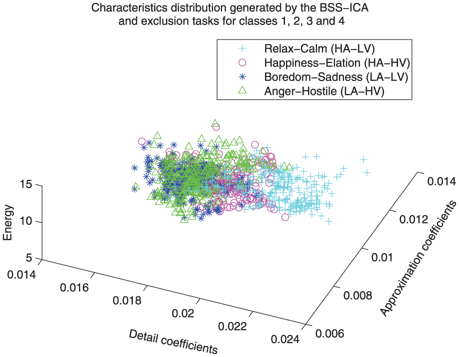
Distribution comparison between all classes. This representation shows the level of complexity for the four-class identification process (class 1: happiness/elation, class 2:anger/hostile, class 3: relaxation/calm, class 4: boredom/sadness).
Implementation of class three as reference
Figures 9, 11 and 10 show feature distribution models that implement class 3 as reference. A very weak correlation between classes 2, 4 and 3 can be observed, while a sightly higher correlation can be observed for classes 1 and 3 (i.e. the relaxation state is more related to happiness than to anger or sadness).
Implementation of class one as reference
Figures 12 and 13 show the feature distribution models that implement class 1 as reference. It can be observed that the correlation between classes 1 and 4 could be considered weak, while the correlation between classes 1 and 2 could be considered strong (i.e. the happiness state is more related to anger than to sadness).
Implementation of class two as reference
Figure 14 shows a feature distribution model that provides a comparison of classes 2 and 4; the relationship between these emotional states is considered very close.
Implementation of a three-classe comparison
In Figures 15 and 16 it can be seen that even though there is clearly overlap between classes, they are mostly distinguishable to the naked eye, except for those combinations labeled with a close relationship, such as anger and sadness.
Implementation of a four-class comparison
Figure 17 provides an overview of the four emotion recognition process that was implemented in this work; it can be observed that these emotions are closely related and represent a considerable increase in the complexity of identification.
NN performance
The implemented NN obtains up to 98% mean recognition rate for the trivial case (by recognizing a single emotional state), while for the binary and the multi-class scheme (two, three and four emotions) the mean identification rates were up to 90.2%, 84.2% and 80.9%, respectively.
The performance of the NN for the two classes recognition process can be observed in Figures 18 and 19, in which can be appreciated the recognition rate by class and a graph showing ten validations, showing a stable performance.
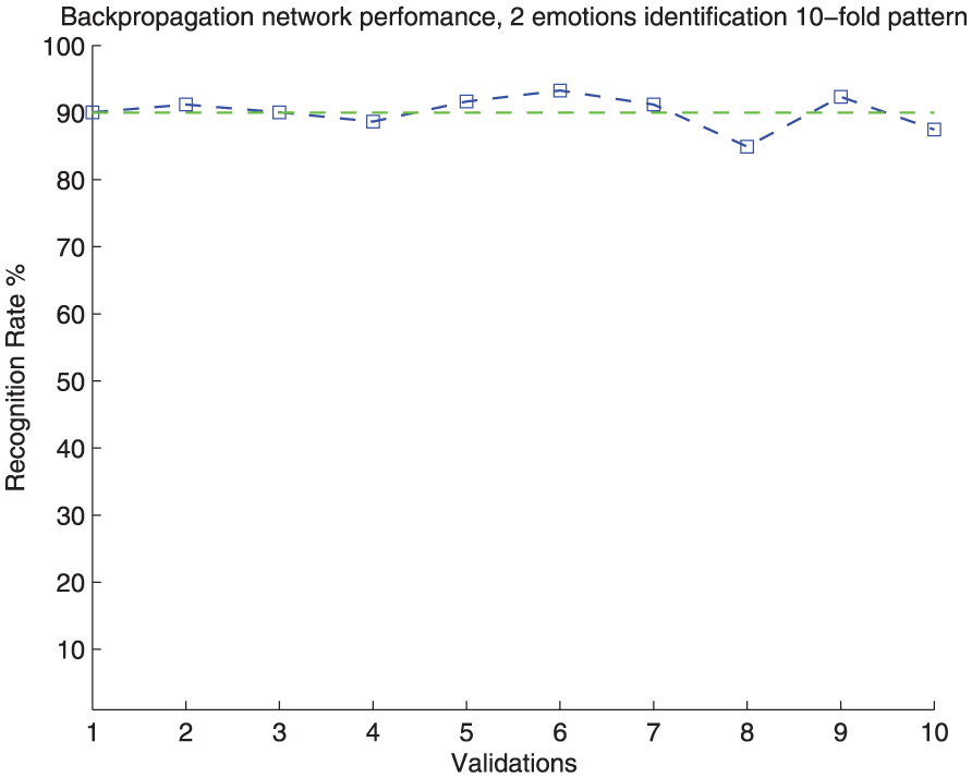
The 10-fold cross-validation performance of the NN for the two-class identification process.
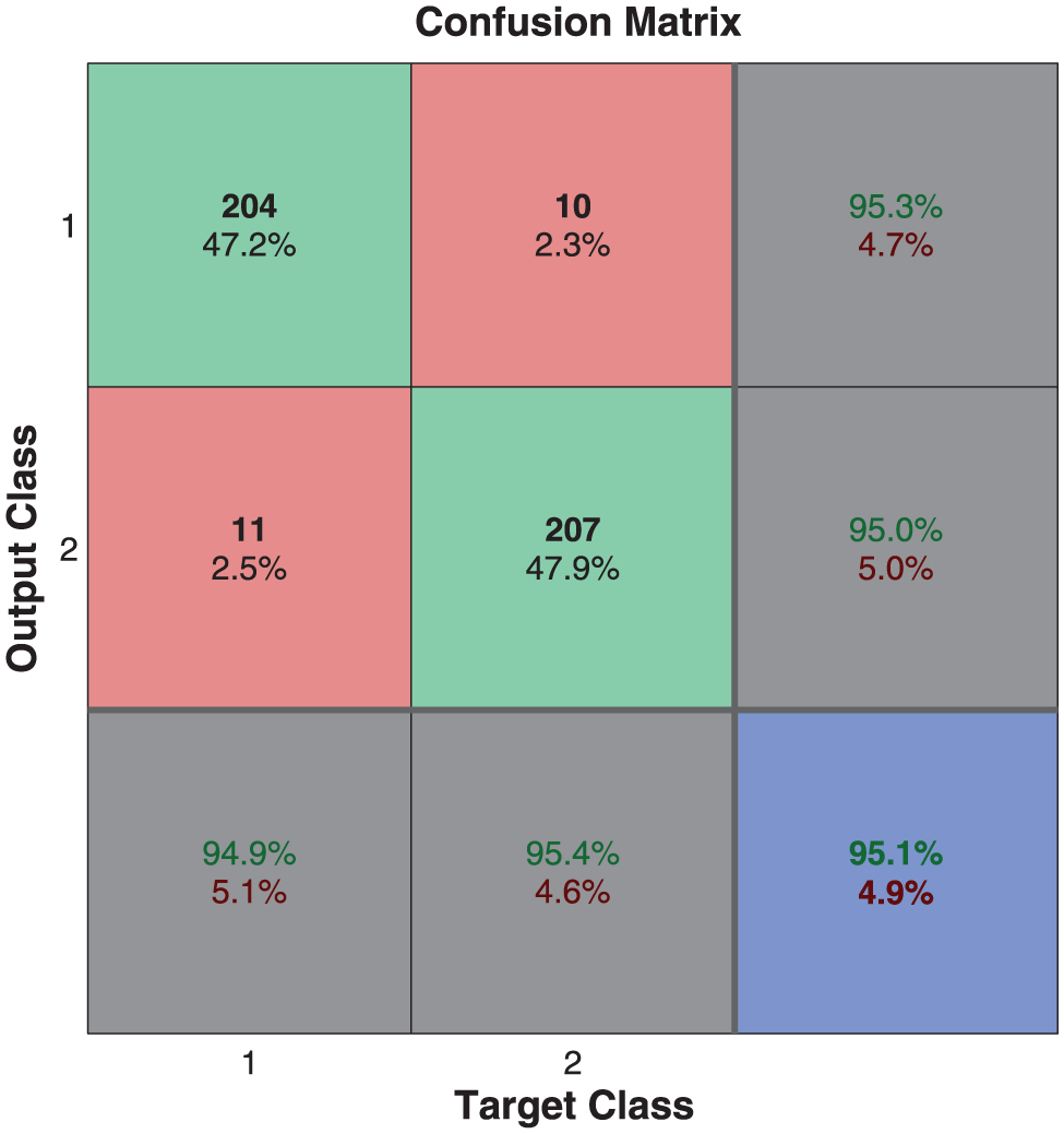
Performance of the NN for the two-class identification process.
Figures 20 and 21 present the identification performance for the three-class recognition scheme, which obtains up to an 84.2% mean identification rate and the 10-fold cross-validation process to evaluate the stability of this identification scheme.
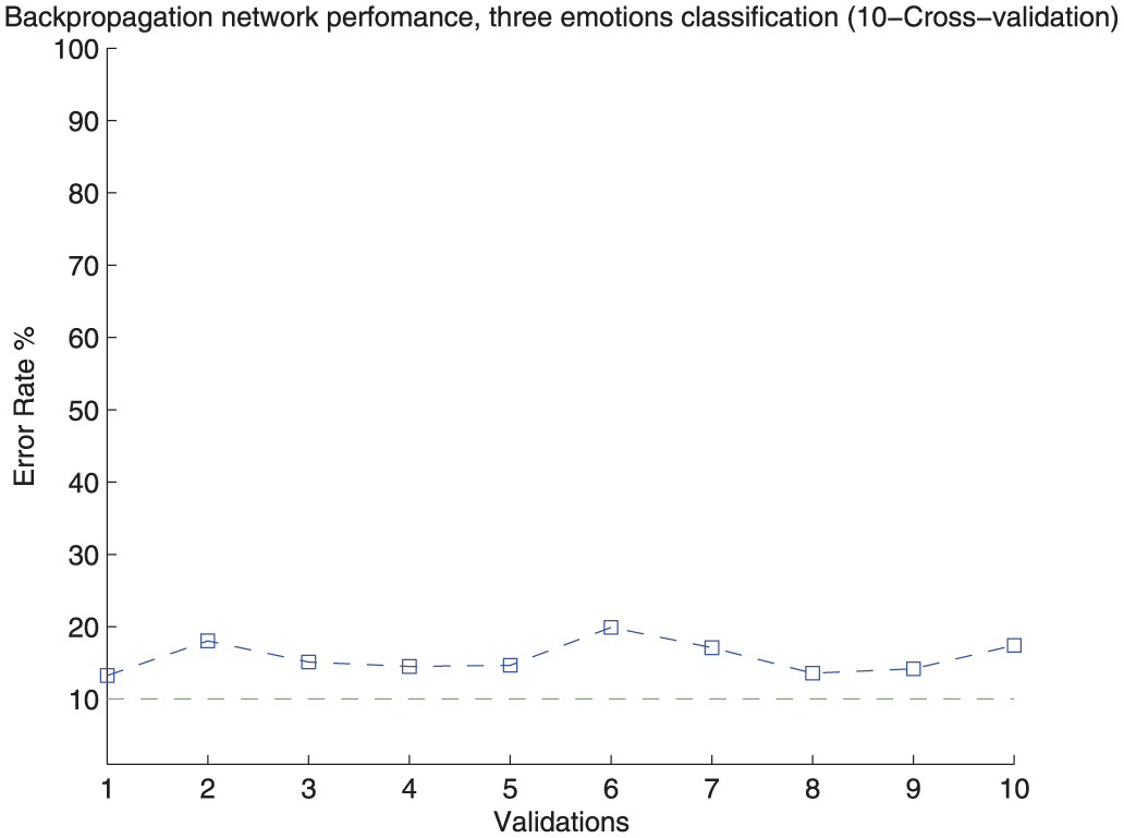
The 10-fold cross-validation performance of the NN for the three-class identification process.
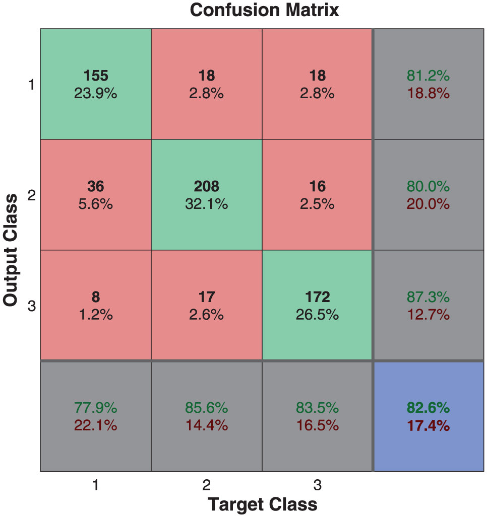
Performance of the NN for the three-class identification process.
Figures 22 and 23 presents the four-class recognition scheme which obtains up to an 80.9% mean identification rate and the 10-fold cross-validation process to evaluate the stability of this identification scheme.
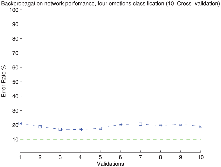
The 10-fold cross-validation performance of the NN for the four-class identification process.
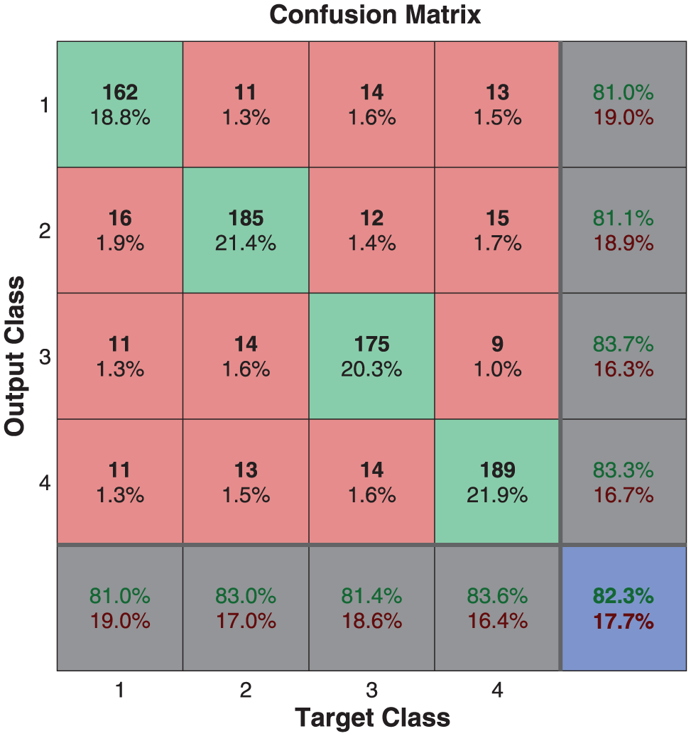
Performance of the NN for the four-class identification process.
SVM performance
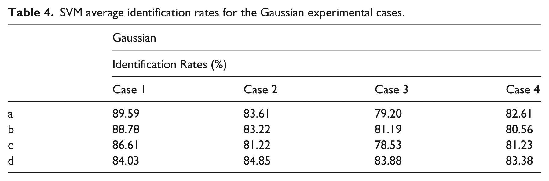
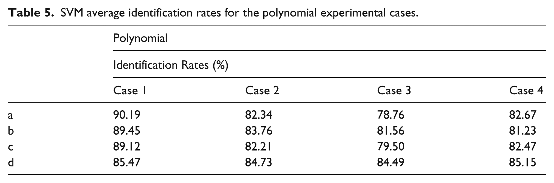
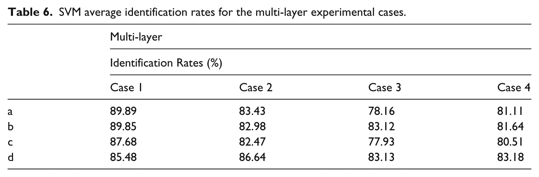
The results obtained by implementing the support vector methodology and the proposed signal conditioning strategy are shown in Tables 4, 5 and 6.
SVM average identification rates for the Gaussian experimental cases.
SVM average identification rates for the polynomial experimental cases.
SVM average identification rates for the multi-layer experimental cases.
SVM identification performance
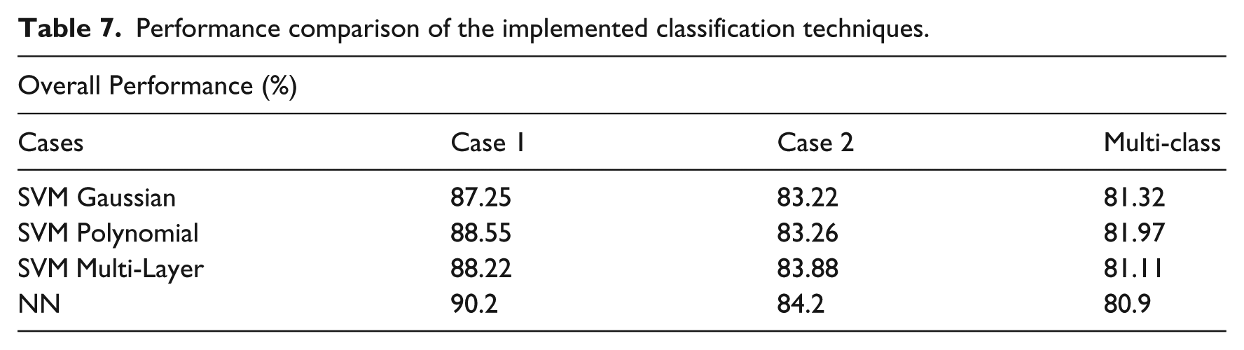
As can be observed in Table 7, the performance obtained from implementing this identification technique and the proposed signal conditioning strategy remains in competitive range when compared with the rates reported in the literature, although it could be considered that some other authors obtain slightly higher identification rates,9,13 despite the fact that their implementations do not consider multi-class problems, while works that do consider multi-class schemes obtain significantly lower identification rates than those presented in this paper.4,5
Performance comparison of the implemented classification techniques.
Conclusions
We present a strategy to carry out an emotion identification process, by analyzing the electroencephalographic activity of users when they are experiencing one or more emotional stimuli by implementing a strategy that reduces the amount of electrodes that have to be analyzed, which can be translated as an a priori removal of large amounts of information from the outset, retaining competitive recognition rates. In addition, some considerations that allow for the reduction of the computational burden required for the recognition and identification process are presented.
Most of the comparatives representations presented in this work contain information sets of up to 16 participants, and for all of them the information appears to be grouped into classes, which suggest the existence of relationships between the signal behavior of emotional states.
Another important aspect that may be noticed is that even though the amount of the initial information is reduced, we did not get any significant penalty in the recognition rates and our identification rates are comparable to those presented by some of the most important researchers in the field, such as Dr Muruarapan. However, the lack of a standard methodology to perform an emotion recognition task is one of the main problems that we faced in the development of this research, since most works implement distinct approaches and even distinct data sources, resulting in a very wide range of experimental procedures and results, making comparison between them unfeasible. The proposals presented by Dr Muruarapan and Dr Scherer underpin the efforts of the community by supporting the importance of affective computing and its impact on technological developments. Also the development of affective computing techniques are becoming more viable with the development of a wide variety of portable devices which facilitate information gathering processes, as well as digital processing techniques.
Because we work with a group of specialists focused on the physical rehabilitation of high performance athletes, the implementation of this algorithm in a real-time platform, combined with a micro-expressions recognizing technique is contemplated as future work to serve as a support tool to monitor patient progress. This is important because experts suggest that some of the athletes endanger their physical integrity, whether by their competitive desire or by frustration. Also almost any modern device has capability to collect and process large amounts of information, and therefore the possibility of developing systems to recognize the emotional states of a user is of growing interest.
Footnotes
Acknowledgements
I would like to thank CONACYT for making this project possible and the Technological Institute of Tijuana for providing necessary technical support for the implementation of this project.
Declaration of Conflicting Interests
The author(s) declared no potential conflicts of interest with respect to the research, authorship, and/or publication of this article.
Funding
The author(s) received no financial support for the research, authorship, and/or publication of this article.