A full numerical solution to the coupled cam–roller and roller–pin contact in heavily loaded cam–roller follower mechanisms

Abstract

In cam–roller follower units two lubricated contacts may be distinguished, namely the cam–roller contact and roller–pin contact. The former is a nonconformal contact while the latter is conformal contact. In an earlier work a detailed transient finite line contact elastohydrodynamic lubrication model for the cam–roller contact was developed. In this work a detailed transient elastohydrodynamic lubrication model for the roller–pin contact is developed and coupled to the earlier developed cam–roller contact elastohydrodynamic lubrication model via a roller friction model. For the transient analysis a heavily loaded cam–roller follower unit is analyzed. It is shown that likewise the cam–roller contact, the roller–pin contact also inhibits typical finite line contact elastohydrodynamic lubrication characteristics at high loads. The importance of including elastic deformation for analyzing lubrication conditions in the roller–pin contact is highlighted here, as it significantly enhances the film thickness and friction coefficient. Other main findings are that for heavily loaded cam–roller follower units, as studied in this work, transient effects and roller slippage are negligible, and the roller–pin contact is associated with the highest power losses. Finally, due to the nontypical elastohydrodynamic lubrication characteristics of both cam–roller and roller–pin contact numerical analysis becomes inevitable for the evaluation of the film thicknesses, power losses, and maximum pressures.

Introduction

Cam–roller follower mechanisms as part of fuel injection units in heavy-duty diesel engines are subjected to very high fluctuating loads coming from the fuel injector. Apart from the high fluctuating contact forces, varying radius of curvature and lubricant entertainment velocity make the tribological design of these components even more challenging. The lubricant entrainment speed of the cam–roller contact on itself is a function of geometrical configuration, cam rotational velocity, and roller angular speed. Two lubricated contacts may be distinguished when considering a cam–roller follower unit, namely the cam–roller contact and roller–pin contact (see Figure 1). The former is a nonconformal contact while the latter is conformal contact. The roller angular speed is a function of the working frictional forces at the cam–roller and roller–pin contact and inertia torque caused by angular acceleration of the roller itself. Roller slip is defined as the difference between the cam and roller surface velocities at the point of contact.

Figure 1.

Cam–roller follower configuration showing the frictional forces acting at the cam–roller and roller–pin contact.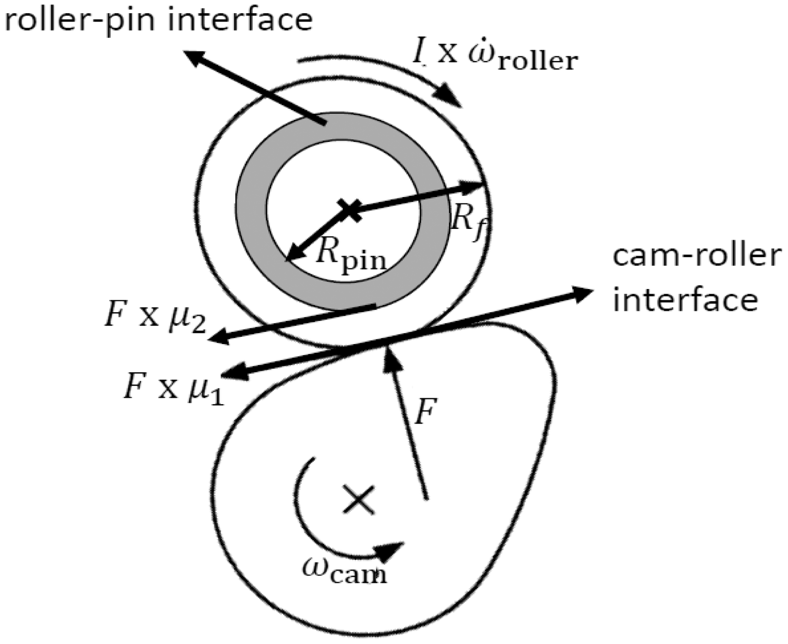

Khurram et al. ¹ proved the existence of roller slip experimentally. Lee and Patterson ² showed that the problem of wear on the interacting surfaces still occurs if slip is present.

Previously developed cam–roller follower lubrication models (see, for instance Chiu, ³ Ji and Taylor, ⁴ and Turturro et al. ⁵ ), which include the possibility of roller slippage, all rely on (semi)-analytical formulations for the film thickness distribution in the cam–roller contact. In those studies the frictional forces working at the roller–pin contact were also estimated using simple analytical formulas or were considered to be constant throughout the whole operating range.

Recently, Alakhramsing et al. ⁶ presented a finite element method (FEM)-based cam–roller lubrication model taking into account axial surface profiling of the roller and also allowing for roller slip. The importance of taking into account axial surface profiling into elastohydrodynamic lubrication (EHL) models has been shown by a number of published studies (see, for instance Wymer and Cameron, ⁷ Shirzadegan et al., ⁸ and Alakhramsing et al. ⁹ ).

The general framework of the model developed in Alakhramsing et al. ⁶ relies on a finite length line contact EHL model for the cam–roller contact and semianalytical lubrication model for the roller–pin contact. The roller–pin contact was modeled as a full film journal bearing. The basis of the semianalytical model used for the roller–pin contact relies on the assumption that the interacting surfaces are rigid and that the lubricant has an isoviscous behavior.

It is expected that under the extremely high contact forces (ranging from 2 to 15 kN), which are also directly transmitted to the roller–pin contact, the “rigid surfaces” assumption might not be accurate. It is therefore important to include elastic deformation of the roller and pin into the analysis. As shown in past studies (see, e.g. O’Donoghue et al. ¹⁰ and Fantino and Frene ¹¹ ) the rigid hydrodynamic solution for journal bearings might significantly overestimate the maximum pressure and underestimate the minimum film thickness.

Therefore, in this paper we present full transient numerical EHL solutions for both cam–roller and roller–pin contact. Both EHL models for cam–roller and roller–pin contact are interlinked via a roller friction model, which predicts possible roller slippage. It is expected that with this model the estimation of important design variables for both cam–roller and roller–pin contact (such as minimum film thicknesses, maximum pressures, and friction losses) is significantly improved and thus leading to a better understanding of the tribological behavior of the cam–roller follower unit. Typical simulation results analyzed in this work are the evolution of the minimum film thickness, maximum pressure, individual frictional losses, and roller slippage along the cam surface.

Mathematical model

The complete mathematical model consists of two FEM-based EHL models corresponding to the cam–roller and roller–pin contact, which are interlinked through the torque balance applied to the roller. Furthermore, it is assumed that thermal effects are insignificant and thus isothermal conditions are assumed.

The first part of the mathematical model, which applies to the cam–roller contact is similar to the full transient EHL solution presented by Alakhramsing et al. ⁶ Hence, in this paper only the main features corresponding to the cam–roller contact are recalled and for further details the reader is asked to refer to Alakhramsing et al. ⁶

The second part of the mathematical model corresponds to the conformal roller–pin contact and relies on a full transient EHL solution for elastic bearings.

Finally, in the last part of this mathematical section the coupling between the two aforementioned EHL models is explained.

Cam–roller contact EHL model

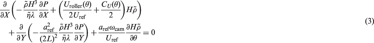
The typical governing EHL equations which apply to the cam–roller contact consist of the Reynolds equation, the load balance equation, and the 3D-linear elasticity equations.

All governing EHL equations for the cam–roller contact are presented in nondimensional form. Hence, the following dimensionless variables are introduced

$$\begin{array}{c}X=\frac{x}{a_{\text{ref}}}Y=\frac{y}{2L}Z=\frac{z}{a_{\text{ref}}}\\ P=\frac{p}{p_{\text{h}}}\stackrel{\sim }{\eta }=\frac{\eta }{{\eta }_0}\stackrel{\sim }{\rho }=\frac{\rho }{{\rho }_0}\\ H=\frac{{\mathit{hR}}_{\text{ref}}}{a_{\text{ref}}^2}{H}_0=\frac{h_0{R}_{\text{ref}}}{a_{\text{ref}}^2}\\ C_R(\theta )=\frac{R_x(\theta )}{R_{\text{ref}}}\\ C_U(\theta )=\frac{U_{\text{cam}}(\theta )}{U_{\text{ref}}}\\ C_F(\theta )=\frac{F(\theta )}{F_{\text{ref}}}G=\frac{{\mathit{gR}}_{\text{ref}}}{a_{\text{ref}}^2}\\ \stackrel{\sim }{\delta }=\frac{\delta R_{\text{ref}}}{a_{\text{ref}}^2}\theta ={\omega }_{\text{cam}}t\end{array}$$

(1)

with Hertzian parameters defined as follows

$$\begin{array}{c}{p}_{\text{h}}=\frac{2F_{\text{ref}}}{\pi {\mathit{La}}_{\text{ref}}}\mathrm{\hspace{1em}\hspace{1em}\hspace{1em}\hspace{1em}\hspace{1em}\hspace{1em}}{a}_{\text{ref}}=\sqrt{\frac{8F_{\text{ref}}{R}_{\text{ref}}}{\pi \mathit{LE}\text{'}}}\\ E\text{'}=\frac{2}{\frac{1-{\nu }_{\text{cam}}^2}{E_{\text{cam}}}+\frac{1-{\nu }_{\text{roller}}^2}{E_{\text{roller}}}}\end{array}$$

(2)

where the subscript “ref” denotes the reference operating conditions.

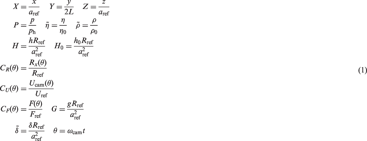
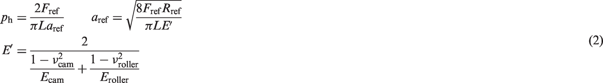
Figure 2 presents the equivalent EHL computational domain Ω for the cam–roller contact. Instead of calculating the elastic deformation twice for the two semi-infinite bodies, an equivalent elastic domain Ω (with equivalent mechanical properties) is chosen for calculation of the combined elastic displacement field $\stackrel{\sim }{\delta }$ (see Habchi et al. ¹² for more details). The dimensionless side length of 60 for the elastic domain Ω is chosen in such a way so that the zero displacement boundary condition, imposed on bottom boundary ${\Omega }_{\text{D}}$ , holds. ¹² ${\Omega }_{\text{f}}$ denotes the fluid domain on which the Reynolds equation is solved and has dimensions of $-4.5\le X\le 1.5$ and $-1\le Y\le 1$ . In the present study the advantage of symmetry (around symmetrical plane ${\Omega }_{\text{s}}$ ) has been taken in order to reduce the computational power required. The dimensionless transient Reynolds equation, which governs the pressure distribution in the contact, is written as follows

$$\begin{array}{c}\frac{\partial }{\partial X}(-\frac{\stackrel{\sim }{\rho }{H}^3}{\stackrel{\sim }{\eta }\lambda }\frac{\partial P}{\partial X}+(\frac{U_{\text{roller}}(\theta )}{2U_{\text{ref}}}+\frac{C_U(\theta )}{2})H\stackrel{\sim }{\rho })\\ +\frac{\partial }{\partial Y}(-\frac{a_{\text{ref}}^2}{(2L{)}^2}\frac{\stackrel{\sim }{\rho }{H}^3}{\stackrel{\sim }{\eta }\lambda }\frac{\partial P}{\partial Y})+\frac{a_{\text{ref}}{\omega }_{\text{cam}}}{U_{\text{ref}}}\frac{\partial H\stackrel{\sim }{\rho }}{\partial \theta }=0\end{array}$$

(3)

where $\lambda =\frac{12U_{\text{ref}}{\eta }_0{R}_{\text{ref}}^2}{a^3{p}_{\text{h}}}$ is the dimensionless speed parameter, and $\stackrel{\sim }{\eta }$ and $\stackrel{\sim }{\rho }$ are the dimensionless viscosity and density of lubricant, respectively. $\theta ={\omega }_{\text{cam}}t$ is the cam angle and ${\omega }_{\text{cam}}$ is the cam rotational speed. $C_U(\theta )$ represents the variation of the cam surface velocity $U_{\text{cam}}$ . Note that $U_{\text{cam}}$ and $U_{\text{roller}}$ are parallel to the x-axis, which is why the wedge term in y-direction in the Reynolds equation is nil. Equation (3) includes the following features/assumptions:

• Compressibility and piezoviscous behavior of the lubricant are modeled using the Dowson–Higginson ¹³ and Roelands ¹⁴ relations, respectively.

• The free boundary problem arising at the outlet of the contact is treated using the penalty formulation of Wu ¹⁵

• Suitable numerical stabilization techniques, as detailed in Habchi et al., ¹² are utilized in order to stabilize the solution at high loads.

• Fully flooded conditions are assumed at the inlet of the contact and opposing surfaces are assumed to be smooth.

Figure 2.

Equivalent geometry for EHL analysis of the finite line contact problem. Dimensions are exaggerated for the sake of clarity.

The film thickness for the cam–roller contact, at any cam angle θ, can be described using the following expression

$$H(X,Y,\theta )=H_0(\theta )+\frac{X^2}{2C_R(\theta )}+G(Y,\theta )-\stackrel{\sim }{\delta }(X,Y,\theta )$$

(4)

where H₀ is the rigid body displacement and $\stackrel{\sim }{\delta }$ is the combined elastic deformation, of which the calculation is based on a 3D-elasticity matrix. ⁶ $C_R(\theta )$ denotes the dimensionless variation of the reduced radius of curvature $R_x=(\frac{1}{{\rho }_{\text{cam}}}+\frac{1}{R_{\text{f}}}{)}^{-1}$ . ${\rho }_{\text{cam}}$ is the cam radius of curvature. $G(Y,\theta )$ is a dimensionless function that represents the axial surface profile of the roller. The roller, considered in this study, has a logarithmic axial shape which is described using the following equation ¹⁶

$$g(y,\theta )=-A\mathit{ln}\{1-[1-\text{exp}(\frac{-z_{\text{m}}}{A})](\frac{2y-L_{\text{s}}}{L-L_{\text{s}}}{)}^2\}$$

(5)

where A represents the degree of crowning curvature, $z_{\text{m}}$ is the crown drop at the extremities, and $L_{\text{s}}$ is the straight roller length. Please note that here only the positive Y-part of the solid domain has been retained to account for the problem symmetry. Furthermore, $g(y,\theta )$ is only valid for $\frac{L_{\text{s}}}{2}\le y\le \frac{L}{2}$ , otherwise zero.

The rigid body displacement H₀ is obtained by satisfying the load balance. In equation form this yields

$${\int }_{{\Omega }_f}2P(X,Y,\theta )\text{d}X=\pi C_F(\theta )$$

(6)

where $C_F(\theta )$ denotes the dimensionless variation of contact force F. Note that the pressure P in equation (6) is multiplied with a factor of 2 in order to account for the symmetry of the problem. The boundary conditions for the complete cam–roller EHL model are summarized as follows: ⁸

• The pressure at the borders of the fluid flow domain Ω _f equals zero.

• Symmetrical boundary conditions are imposed at plane ${\Omega }_{\text{s}}$ for the elastic and hydrodynamic problem.

• A zero displacement condition is imposed at bottom boundary ${\Omega }_{\text{D}}$ .

• For the elastic part a pressure boundary condition is imposed on the fluid flow domain Ω _f .

• On all remaining boundaries zero stress conditions are imposed.

Finally, the friction coefficient ${\mu }_{\text{cam}-\text{roller}}$ defined at the cam–roller contact is calculated as follows

$$\begin{array}{c}{\mu }_{\text{cam}-\text{roller}}=\frac{2L{\eta }_0{R}_{\text{ref}}}{a_{\text{ref}}F}{\int }_{{\Omega }_f}\frac{\stackrel{\sim }{\eta }(U_{\text{roller}}-U_{\text{cam}})}{H}\\ +\frac{2{\mathit{La}}_{\text{ref}}^2{p}_h}{R_{\text{ref}}F}{\int }_{{\Omega }_f}\frac{H}{2}\frac{\partial P}{\partial X}\text{d}\Omega \end{array}$$

(7)

Roller–pin contact EHL model

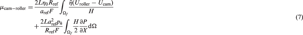
Figure 3 shows the configuration of the roller–pin bearing. The roller is free to rotate and the pin is fixed to the tappet around the inner circumference of the so-called ears of the tappet. In between the roller and the ears of the tappet a small clearance is kept in order to allow the roller to freely rotate and also to allow lubricant to reach the roller–pin interface through the sides of the contact. Figure 4 shows the deduced computational domain for the roller–pin EHL model shown in Figure 3. As can be extracted from this figure the advantage of symmetry has been taken at the y = 0 plane. Unlike for the cam–roller contact, the governing equations for the roller–pin contact are solved in dimensional form.

Figure 3.

Example of a cam–roller follower unit.

Figure 4.

Roller–pin contact computational domain. Dimensions are exaggerated for the sake of clarity.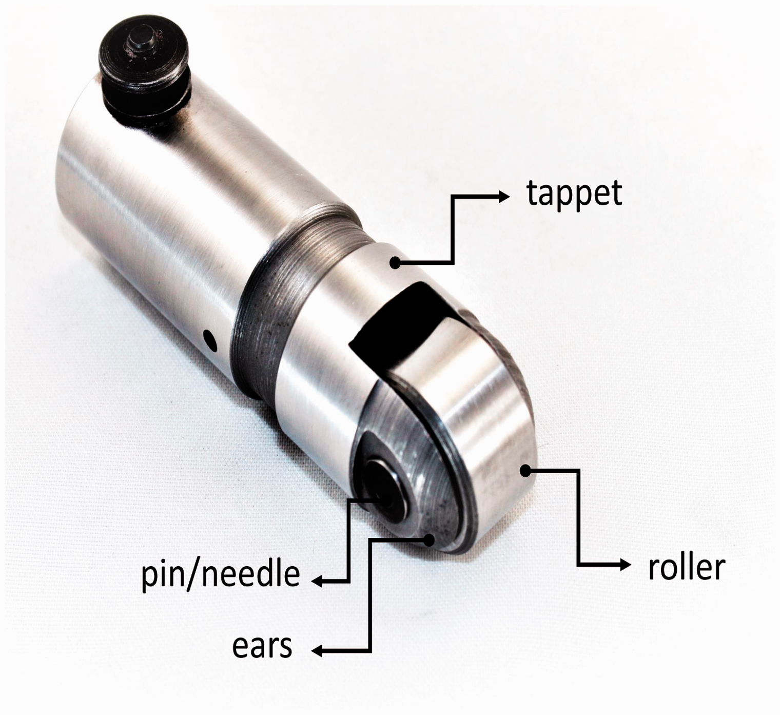

The pin is slightly crowned in axial direction in order to reduce edge stress concentrations, while the roller inner surface is assumed to be perfectly straight. The film thickness distribution for the roller–pin contact, which can be described in similar manner as for an elastic journal bearing, is written as follows

$$h=C-e_{\overline{x}}\text{cos}\Theta -e_{\overline{y}}\text{sin}\Theta +\frac{y^2}{2R_y}+{\partial }_{\text{r}}$$

(8)

where C is the nominal radial clearance, R_y is the crowing curvature of the pin, $e_{\overline{x}}$ and $e_{\overline{y}}$ are the global $\overline{x}$ and $\overline{y}$ components of the roller eccentricity (see Figure 5) and ${\partial }_{\text{r}}={\delta }_{\text{roller}}+{\delta }_{\text{pin}}$ is the combined radial elastic deformation of roller and pin. Unlike for rigid bearings, the dimensionless eccentricity $\epsilon =\frac{e}{C}$ is allowed to be greater than one when elastic deformation is taken into account. ¹⁰

Figure 5.

Schematic view of a cylindrical journal bearing with fixed coordinate system (x, y) and moving coordinate system (r, t).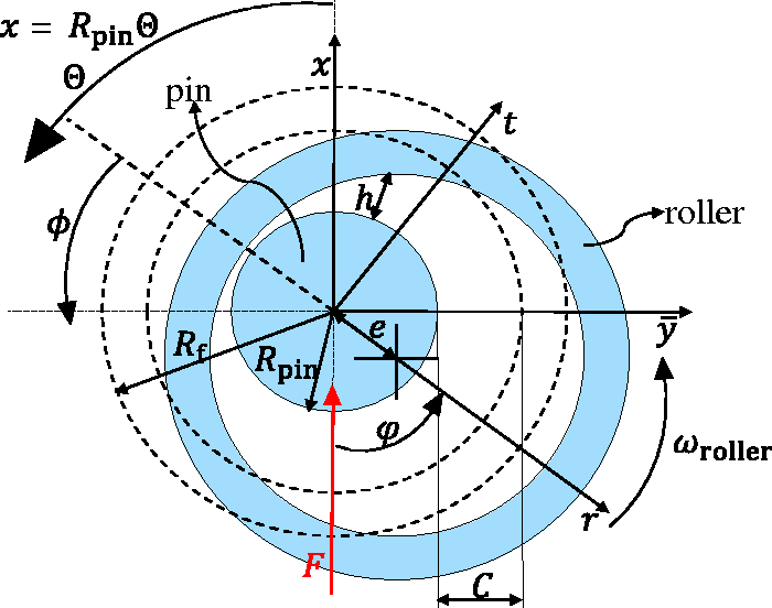

Note that, unlike for the cam–roller contact, the elastic deflections for roller and pin are individually calculated and summed up for evaluation of the film thickness. $\Theta =\phi +\varphi$ is the circumferential coordinate. ϕ is the roller attitude angle, i.e. $e_x=e\text{cos}\varphi$ and $e_y=e\text{sin}\varphi$ . The angle φ is the circumferential coordinate defined as starting from the minimum film thickness $\frac{R_{\text{pin}}{U}_{\text{roller}}}{R_f}$ of the roller–pin bearing (see Figure 5).

The Reynolds equation, which governs the pressure distribution in the roller–pin contact, is written as follows

$$\begin{array}{c}-\frac{1}{R_{\text{pin}}^2}\frac{\partial }{\partial \Theta }(\frac{\rho h^3}{12\eta }\frac{\partial p}{\partial \Theta })-\frac{\partial }{\partial y}(\frac{\rho h^3}{12\eta }\frac{\partial p}{\partial \Theta })\\ +\frac{U_{\text{roller}}}{2R_f}\frac{\partial }{\partial \Theta }(\rho h)+{\omega }_{\text{cam}}\frac{\partial }{\partial \theta }(\rho h)=0\end{array}$$

(9)

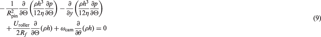
Note that $U_{\text{roller}}$ is the outer roller surface velocity, while $\frac{R_{\text{pin}}{U}_{\text{roller}}}{R_f}$ is the inner roller surface velocity.

Similar to the cam–roller contact, variation of viscosity and density with pressure is simulated using the Roeland’s ¹⁴ and Dowson–Higginson ¹³ rheological expressions. The cavitation problem within the lubricated contact is treated according to the penalty formulation of Wu. ¹⁵

In the present analysis we align the x-axis of the (x, y) coordinate system at all times with force vector $F(\theta )$ , which acts at the cam–roller contact (see Figure 5). The eccentricity components $(e_x,e_y)$ are obtained by satisfying the equations of motion

$$\begin{array}{c}{m}_{\text{roller}}{\omega }_{\text{cam}}^2[\begin{array}{c}{\stackrel{\mathrm{··}}{e}}_{\overline{x}}\\ {\stackrel{\mathrm{··}}{e}}_{\overline{y}}\end{array}]=[\begin{array}{c}{F}_x\\ F_y\end{array}]-[\begin{array}{c}F\\ 0\end{array}]\end{array}$$

(10)

where the fluid film reaction forces are defined as follows

$$\left[\begin{array}{c}{F}_x\\ F_y\end{array}\right]={\displaystyle \underset{-L/2}{\overset{L/2}{\int }}{\displaystyle \underset{0}{\overset{2\pi }{\int }}p\left(\Theta ,y,\theta \right)}}\left[\begin{array}{c}\cos \Theta \\ \sin \Theta \end{array}\right]R_{\text{pin}}·d\Theta dy$$

(11)

Note that due to the unique definition of coordinate system (x, y) the y-component of the applied load F is zero at all times. The radial displacement ${\partial }_{\text{r}}$ , which is caused by the lubricant pressure buildup in the contact, is evaluated using a full deformation model based on a 3D-elasticity matrix. ¹⁷

The boundary conditions for the complete roller–pin EHL model are summarized as follows:

The pressure is continuous and periodic in circumferential direction Θ.

A zero pressure condition is imposed at the (side) borders of the fluid film domain in order to simulate fully submerged conditions.

A zero displacement condition is imposed at the common interface between the pin and inner surface of the ears of the tappet.

For the elastic part a pressure boundary condition is imposed on the outer surface of the pin and inner surface of the roller on the lubricant flow domain.

The center of contact between the cam and roller always lies on the x-axis of the roller–pin model. The most accurate way to describe the boundary condition at the outer surface of the roller, where cam–roller contact occurs, would be by prescribing the displacement field which is calculated from the cam–roller contact EHL model. However, from our simulations we observed that similar results are obtained if a zero displacement condition is imposed on the outer contact domain. Of course, the size of the contact domain itself varies for different cam angles (due to varying operating conditions). Nevertheless, based on dry Hertzian analysis an estimation of the range in which the contact area varies can be made. For the cases studied, the contact width varies between 0.3 and 0.6 mm. Due to the considerably large thickness of the roller, the displacement fields of cam–roller and roller–pin contact are not at all influenced by each other. So, for the current analysis a fixed outer roller boundary has been used at all cam angles on which a zero displacement condition has been imposed.

On all remaining boundaries zero stress conditions are imposed.

Finally, the friction coefficient ${\mu }_{\text{roller}-\text{pin}}$ defined at the roller–pin contact is calculated as follows

$$\begin{array}{l}{\mu }_{\text{roller-pin}}={\displaystyle \underset{-L/2}{\overset{L/2}{\int }}{\displaystyle \underset{0}{\overset{2\pi }{\int }}-\frac{h}{2F{R}_{\text{pin}}}\frac{dp}{d\Theta }}}\hfill \\ +\eta \frac{R_f}{F{R}_{\text{pin}}}\frac{U_{\text{roller}}}{h}{R}_{\text{pin}}·d\Theta dy\hfill \end{array}$$

(12)

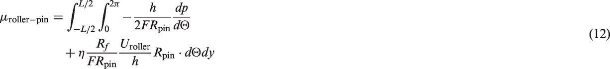
Note that in the current analysis friction evaluation is based on isothermal and Newtonian assumptions. Extension of the model to capture non-Newtonian and thermal effects is suggested for future work.

Coupling of cam–roller and roller–pin contact

As mentioned earlier, the cam–roller and roller–pin contact are coupled through the global torque balance applied to the roller. The global torque balance used for calculation of roller rotational speed ${\omega }_{\text{roller}}$ yields ⁴

$$\underset{\text{tractivetorque}}{\underbrace{{\mu }_{\text{cam}-\text{roller}}{R}_{f}F}}=\underset{\text{resistingtorque}}{\underbrace{{\mu }_{\text{roller}-\text{pin}}{R}_{\text{pin}}F}}+\underset{\text{inertiatorque}}{\underbrace{I{\omega }_{\text{cam}}{\stackrel{·}{\omega }}_{\text{roller}}}}$$

(13)

where $I=0.5m_{\text{roller}}(R_{\text{pin}}^2+R_f^2)$ is the mass moment inertia of the roller and friction coefficients ${\mu }_{\text{cam}-\text{roller}}$ and ${\mu }_{\text{roller}-\text{pin}}$ are calculated by means of equations (7) and (12), respectively. When the RHS of equation (13) increases, the sliding velocity at the cam–roller contact consequently also needs to increase to satisfy the torque balance, i.e. the LHS needs to increase. This is also known as the “self-correcting action.” ⁴

Overall numerical procedure

The complete models thus consists of two sub-EHL models corresponding to cam–roller and roller–pin contact. The governing equations for both models include the Reynolds equations and the 3D-linear elasticity equations with their associated BCs. Additionally, for the cam–roller EHL model the load balance (with unknown H₀) is added to the system of equations, while for the roller–pin EHL model the equations of motion (with unknown eccentricity components $e_{\overline{x}}$ and $e_{\overline{y}}$ ) are added to the system of equations.

The two submodels are interlinked via the global torque balance, which determines the roller angular velocity ${\omega }_{\text{roller}}$ .

The complete model is solved using a finite element analysis software package. ¹⁷ In fact, the problem is formulated as a set of strongly coupled partial differential equations. After finite element discretization, the resulting set of nonlinear equations is solved using a monolithic approach in which all dependent variables $(\{P,\stackrel{\sim }{\delta },H_0{\}}_{\text{cam}-\text{roller}},\{p,\delta ,e_x,e_y{\}}_{\text{roller}-\text{pin}},{\omega }_{\text{roller}})$ are collected in one vector of unknowns and simultaneously solved using a damped Newton–Raphson iteration scheme.

From a numerical perspective the weak form finite element formulation of the governing EHL equations of both submodels is similar, except from the fact that the computational domains are different. Therefore, for numerical details pertaining the fully coupled approach the reader is referred to Habchi et al. ¹² as only the main features are recalled here.

A similar customized element size distribution, as detailed in Habchi et al., ¹² was employed for the equivalent EHL computational domain for the cam–roller contact.

For the roller–pin contact a similar strategy was followed, i.e. in the pressure buildup region a dense element distribution was chosen which was allowed to decrease gradually as the distance from the fluid film boundary increased.

For both the models Lagrange quintic elements were used for the hydrodynamic part while for the elastic part Lagrange quadratic elements were used. The aforementioned custom-tailored meshes for cam–roller and roller–pin EHL models correspond to approximately 350,000 degrees of freedom in total.

Steady-state solutions were fed as initial guess for the transient calculations. Steady-state solutions are reached within 11 iterations, corresponding to relative errors between ${10}^{-3}\text{ and }{10}^{-4}$ and calculation times ranging from 1.5 to 2 min on a computer with an Intel® Core™ i7-2600 processor.

For the transient calculations a dimensionless time step $\Delta \theta$ of 0.01 was chosen. In regions where abrupt kinematic variations occur smaller time step sizes were chosen.

Results

In this section a comprehensive transient analysis, for the considered cam and roller follower, is performed and the results are presented. The analyzed cam–roller follower unit is part of a fuel injection pump unit of a heavy-duty diesel engine. The operating conditions considered here are similar to those presented in Alakhramsing et al. ⁶ and correspond to a cam rotational speed of 950 r/min. The configuration parameters and reference operating conditions are given in Table 1. Figure 6 presents the dimensionless variation of the cam surface speed, load, and reduced radius of curvature for the cam–roller contact. As explained in Alakhramsing et al. ⁶ the profile for the contact force inhibits abrupt variations, ranging from 2 to 13 kN, which are due to sudden activation and deactivation of pumping action. Furthermore, the cam surface speed and reduced radius of curvature are fairly constant (with minor variations) throughout the cam’s lateral profile. Note that the variations of $C_R(\theta ),C_U(\theta )$ , and $C_F(\theta )$ are identical for $0^{\circ }-{180}^{\circ }$ and ${180}^{\circ }-{360}^{\circ }$ cam angle. Therefore, in this work results are only presented for $0^{\circ }-{180}^{\circ }$ cam angle.

Table 1.

Reference operating conditions and geometrical parameters for cam–roller follower analysis.

Parameter	Value	Unit
$E\text{'}$	220	GPa
ν	0.3	–
α	1.78E-8	Pa−1
η 0	0.01	Pa s
R f	0.018	m
R pin	0.0095	m
C	74	µm
L	0.021	m
Ry	4.5	m
m roller	0.11	kg
A	17	µm
L s	0.007	m
z m	50	µm
R ref	0.015	m
U ref	4.2	m/s
F ref	2250	N

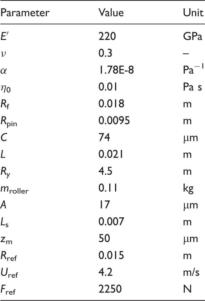
Source: Adopted from Alakhramsing et al. ⁶

Figure 6.

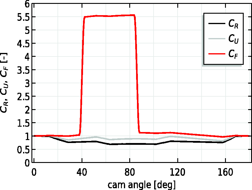
Variation of the dimensionless reduced radius $C_R(\theta )$ , cam surface speed $C_U(\theta )$ , and contact force $C_F(\theta )$ as a function of cam angle θ.

Figures 7 and 8(a) depict height expressions for the pressure distributions in the cam–roller and roller–pin contact at 64° cam angle (cam’s nose region), where the tribological conditions are worst. In both aforementioned figures traditional characteristics corresponding to finite line contact solutions are observed. To be more specific, for the cam–roller contact, which has a logarithmically shaped roller, typical secondary pressure peaks are observed at the sides of the contact. Near the occurrence of the secondary pressure peak, the absolute minimum film thickness $h_{\text{min}}$ is located.

Figure 7.

Height expression of the pressure distribution for cam–roller contact at 64° cam angle. Note that here dimensionless space coordinates (X, Y), as given in equation (1), are used. Furthermore, the dimensions are exaggerated for the sake of clarity.

Figure 8.

Evaluation of pressure and film thickness distribution for the roller–pin contact. The operating conditions correspond to those at 64° cam angle, which lies in the cam’s nose region. (a) Height expression of the pressure distribution. Space coordinates are dimensional here, (b) pressure and film thickness distribution along line Y = 0, and (c) Contour plot of the film thickness distribution illustrating the formation of side lobes.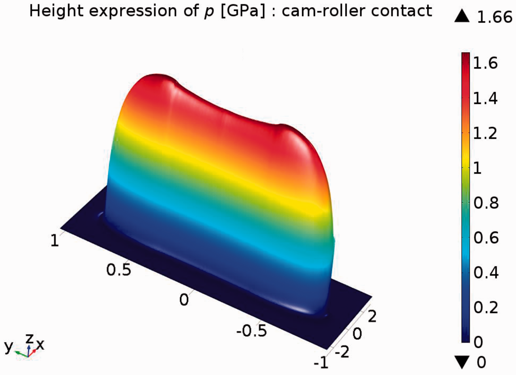

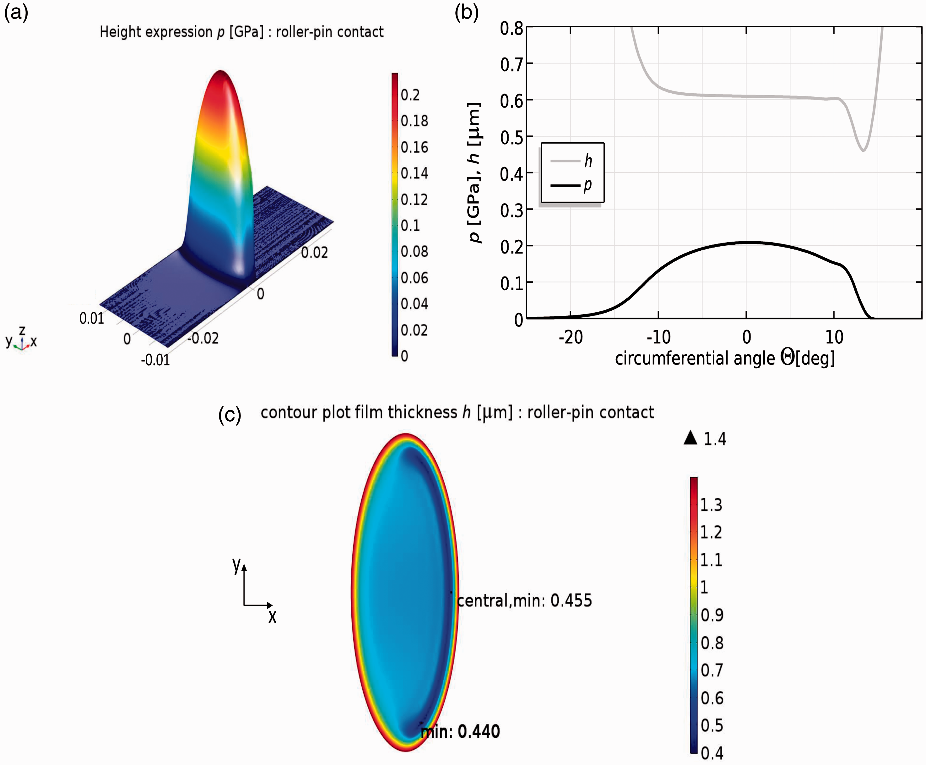
For the roller–pin contact, which has an axially crowned pin, the maximum pressure is located in the central plane (Y = 0). Due to axial crowning of the pin, the contact footprint has an elliptic shape. Figure 8(c) shows the contour plot of the film thickness distribution for 64° cam angle, from which can be extracted that side lobes are formed where minimum film thickness $h_{\text{min}}$ occurs (see Nijenbanning et al. ¹⁸ ).

Figure 8(b) presents the pressure and film thickness distribution for the roller–pin contact at the Y = 0 plane. It can readily be observed that the pressure and film thickness distribution inhibit typical EHL characteristics, i.e. a Hertzian parabolic-type pressure curve and film thickness distribution which is uniform in the center of the contact and has a local restriction $h_{\text{min},\text{central}}$ at the outlet of the contact. Similar findings were reported by O’Donoghue et al. ¹⁰ for elastic journal bearings with high eccentricity ratios. An important remark to make here is that the roller–pin contact may be conformal in nature, but has a similar tribological behavior as nonconformal finite length line contacts for the range of loads considered. In line with this finding, the importance of axial surface profiling of the pin is highlighted here as an axially straight pin might induce edge loading.

Figure 9(a) shows the evolution of minima film thickness as a function of cam angle. Again, note that $h_{\text{min},\text{central}}$ is the central plane (Y = 0) minimum film thickness, while $h_{\text{min}}$ is absolute minimum film thickness which usually occurs at the rear of the contact where axial surface profiling starts. ⁹

Figure 9.

Evolution of minima film thicknesses for (a) cam–roller contact and (b) roller–pin contact.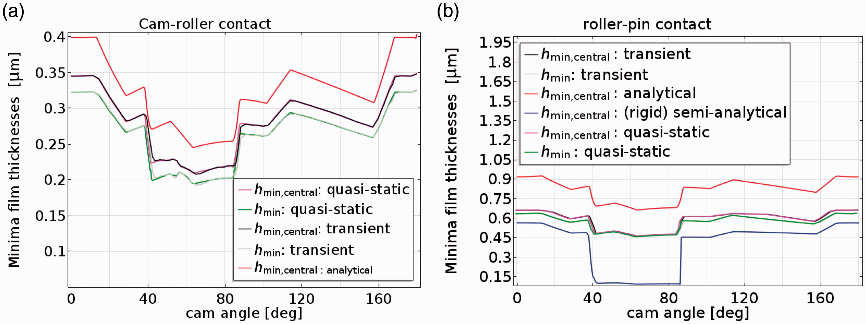

At a first glance one may observe the “dips” in the profiles between ${40}^{\circ }\text{ and }{90}^{\circ }$ cam angle. These are mainly due to the sudden increase in contact force, as the cam surface speed and radius of curvature are fairly constant. Figure 9(a) also compares the results for a full transient solution with those obtained using quasi-static analysis. It can be concluded that transient effects, in this case squeeze film motion, are negligible as a minimal phase lag between the solutions is observed. These findings are in line with past studies^19,20 from which may be concluded that squeeze film effects are mainly important in cases where the entrainment velocity profile inhibits points of flow reversal, i.e. the entrainment velocity profiles passes a zero value. Figure 9(a) also shows the evolution of the minimum film thickness obtained using the Dowson–Higginson ¹³ film thickness equation for infinite line contact. It is clear that the analytical solution significantly overestimates $h_{\text{min},\text{central}}$ as it does not account for side leakage.

Similar observations are made for the roller–pin contact (see Figure 9(b)), i.e. quasi-static analysis yields fairly accurate results as squeeze film motion effects appear to be negligible. For the sake of comparison, Figure 9(b) also depicts the results obtained using the semianalytical model, based on rigid surfaces, as used by Alakhramsing et al. ⁶ It is clear that, especially in the high contact force regions, the minimum film thickness is highly underestimated as elastic deformation is disregarded in this model. In fact, for the rigid surface semianalytical model, the dimensionless eccentricity ratio $\epsilon =\frac{e}{C}$ is not allowed to be larger than one, which leads to calculation of very small film thicknesses. It is apparent from Figure 13 that the dimensionless eccentricity ratio is larger than one throughout the whole operating range. This also highlights the importance of taking into account elastic deformation of roller and pin in the analysis. Finally, if closely noticed, one may observe that the ratio $h_{\text{min}}/h_{\text{min},\text{central}}$ increases in the cam’s nose region. This is mainly due to the fact that with formation of side lobes, where $h_{\text{min}}$ occurs, the ratio $h_{\text{min}}/h_{\text{min},\text{central}}$ is load dependent (see, for instance Alakhramsing et al. ⁹ and Nijenbanning et al. ¹⁸ ).

From Figure 8(b) it can be extracted that the pressure and film thickness distribution in the highly loaded roller–pin contact, which is a conformal contact, inhibits typical EHL features for concentrated nonconformal contacts. The conformal contact in this case may be described by a cylinder with radius $R_{\text{pin}}$ in a hollow outer cylinder with inner radius $R_{\text{pin}}+C$ . For conformal contacts the reduced radius of curvature can be calculated provided that the radius of curvature of the (concave) outer cylinder radius is taken as negative. For the case considered (see Table 1) this would be approximately 1 m. The result for the evolution of $h_{\text{min},\text{central}}$ , after applying the Dowson–Higginson ¹³ film thickness equation for infinite line contacts, for the roller–pin contact is depicted in Figure 9(b). Similar as for the cam–roller contact, the minimum film thickness is significantly overestimated due to nontypical EHL characteristics of finite length line contacts.

Figure 10 presents the evolution of the maximum pressures corresponding to the cam–roller and roller–pin contact. As can be seen, the maximum pressure for the cam–roller contact cycles between 0.65 and 1.75 GPa, while the roller–pin contact experiences significantly lower pressures (ranging between 0.1 and 0.25 GPa). The difference in experienced pressure between cam–roller and roller–pin contact is due to the difference in contact area. As a matter of fact, the contact width for the cam–roller contact varies between 0.2 and 0.6 mm, corresponding to base circle and nose regions, respectively. For the roller–pin contact the contact width varies between 3.8 and 5.8 mm, corresponding to base circle and nose regions, respectively.

Figure 10.

Evolution of the maximum pressures, corresponding to the cam–roller and roller–pin contact, as a function of cam angle θ.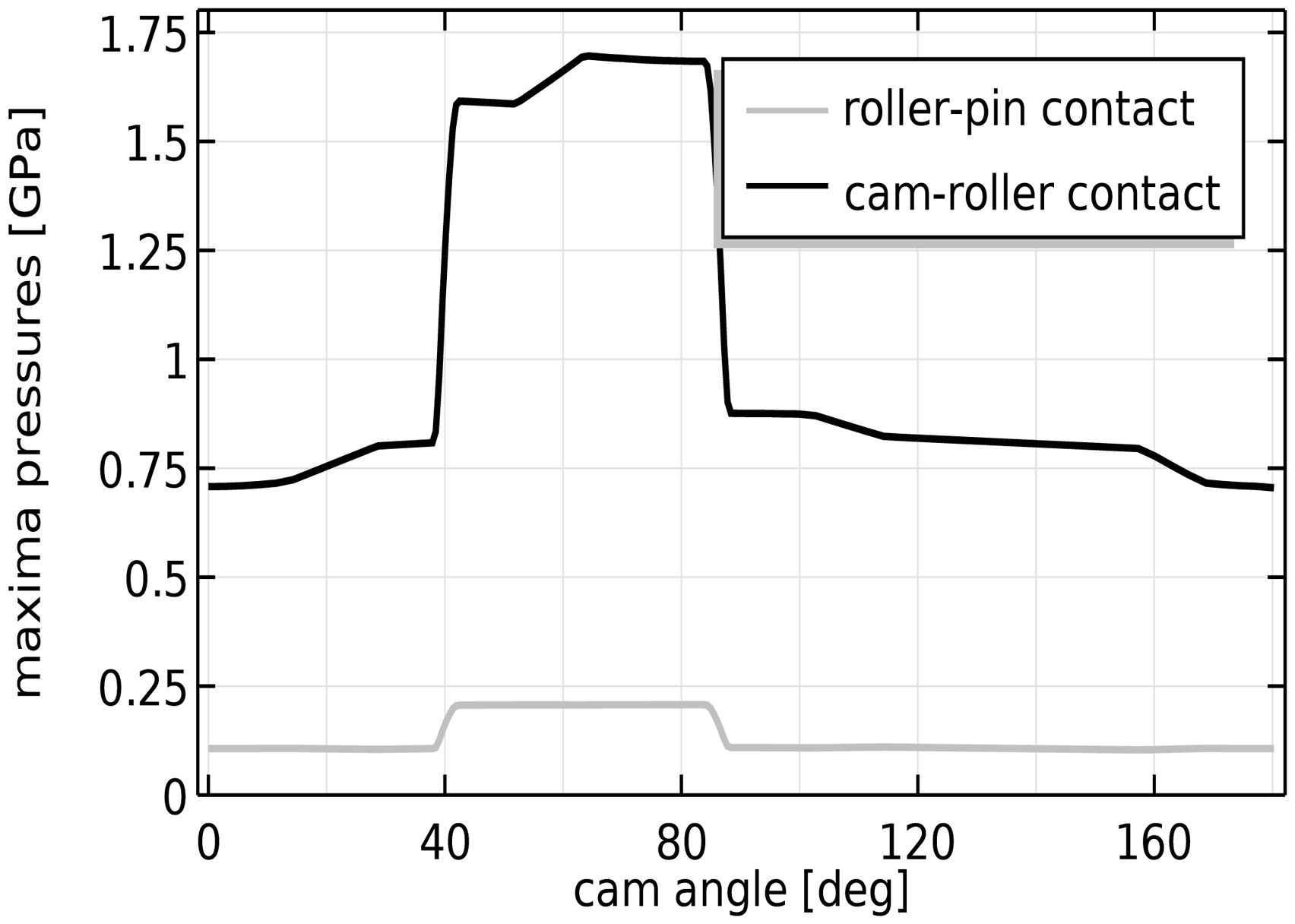

In general, for both contacts the tribological conditions are worst in the cam’s nose region, i.e. both minimum film thickness and maximum pressure occur between ${40}^{\circ }\text{ and }{90}^{\circ }$ cam angle.

The evolution of the slide-to-roll ratio $(\text{SRR})=\frac{U_{\text{cam}}-U_{\text{roller}}}{0.5(U_{\text{cam}}+U_{\text{roller}})}$ , for the cam–roller contact, is depicted in Figure 11. SSR is lowest in the nose region, due to large contact forces, and highest in the base circle regions. Nevertheless, roller slip is negligible throughout the whole cam’s lateral surface due to overall high contact forces and due to the fact that the limiting traction coefficient ${\mu }_{\text{lim}}$ is never exceeded.

Figure 11.

Evolution of the SRR, corresponding to the cam–roller contact, as a function of cam angle θ.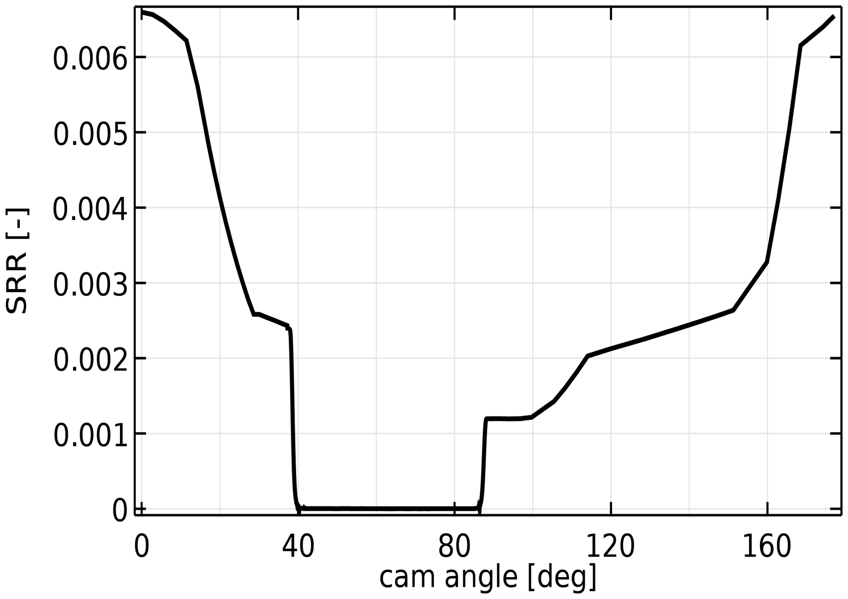

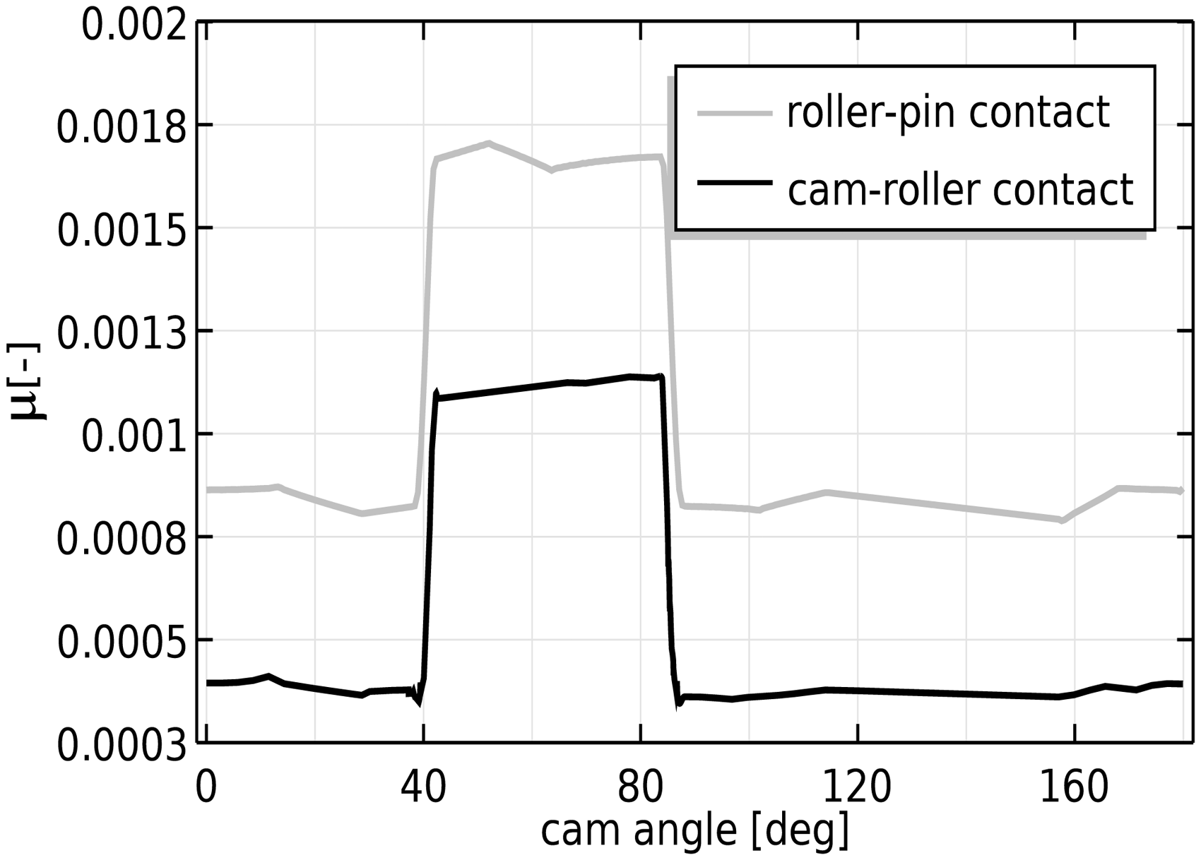
The friction coefficients for cam–roller and roller–pin contact are depicted in Figure 15 from which it can be noticed that very low values of friction coefficients are achieved. The range of values for the roller–pin friction coefficient is of the same magnitude as those measured by Lee and Patterson. ² An increase in friction coefficient is noticed in the nose region. This increase is mainly caused due to a substantial increase in viscosity. Assuming a composite surface roughness of 0.2 µm, it can be inferred that the cam–roller contact operates in the mixed lubrication regime, i.e. $\frac{h}{\sigma }<3$ . This means that the friction coefficient for the cam–roller contact would be higher and the values depicted in Figure 15 should be seen as a minimum. On the other hand, whether the cam–roller contact operates in mixed or full-film regime should not have a large influence on the tribological behavior of the roller–pin contact as operating in mixed lubrication regime of the cam–roller contact will only enhance traction, resulting to less slip. Extension to a mixed lubrication model for both cam–roller and roller–pin contact is suggested for future work.

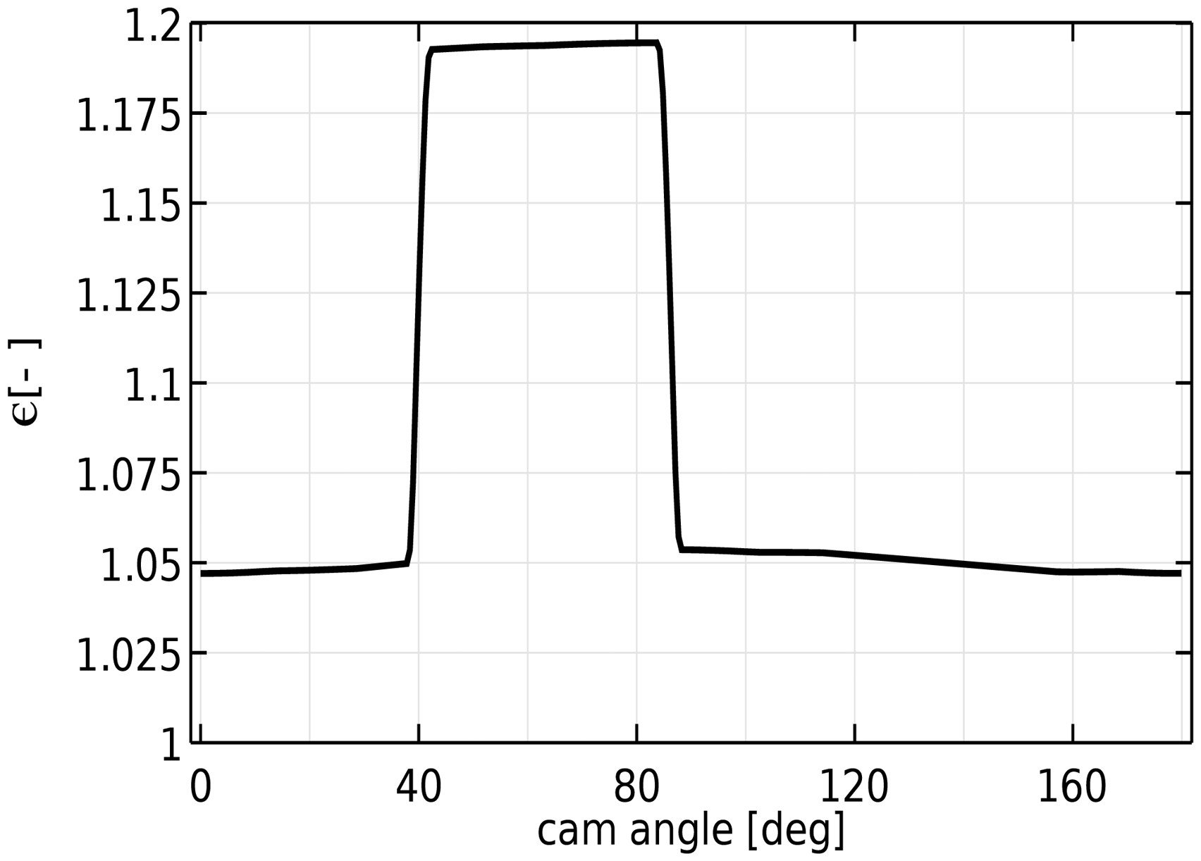
Except from the fact that elastic deformation of roller and pin enhance the film thickness distribution, it is also worth noting that the friction coefficient is also significantly improved for the load range considered. This can be retrieved from Figure 12, which presents ${\mu }_{\text{roller}-\text{pin}}$ as a function of contact force F (and assuming $U_{\text{roller}}$ to be constant). In fact, the ${\mu }_{\text{roller}-\text{pin}}$ is in its optimal range for the load range (2–13 kN) considered. It is obvious that when elastic deformation is considered the contact area increases. Consequently, the hydrodynamic pressure decreases and thus also the sliding frictional force (which is viscosity dependent) decreases. The trend of ${\mu }_{\text{roller}-\text{pin}}$ can be explained as follows. When elastic deformation is insignificant, ${\mu }_{\text{roller}-\text{pin}}$ is inversely proportional to the Sommerfeld number $S=\frac{F}{{\eta }_0{\omega }_{\text{roller}}{\mathit{LR}}_{\text{pin}}}(\frac{C}{R_{\text{pin}}}{)}^2$ (see, for instance Alakhramsing et al. ⁶ ), i.e. ${\mu }_{\text{roller}-\text{pin}}\sim 1/S$ . So, in hydrodynamic lubrication (HL) ${\mu }_{\text{roller}-\text{pin}}$ decreases with increasing loads until the moment when elastic deformation becomes important, i.e. the elastohydrodynamic lubrication (EHL) regime is attained. In pure EHL conditions ${\mu }_{\text{roller}-\text{pin}}$ will increase with increasing loads. So, the load range in which the roller–pin contact operates can be seen as a transition zone from HL to EHL conditions. It is clear from Figure 12 that for loads higher than 10 kN approximately ${\mu }_{\text{roller}-\text{pin}}$ starts increasing again. Meaning that for this case pure EHL conditions are achieved for loads higher than 10 kN approximately.

Figure 12.

Variation of roller–pin contact friction coefficient ${\mu }_{\text{roller}-\text{pin}}$ as a function of applied load F. $U_{\text{rollre}}$ is kept fixed at 4.2 m/s.

Figure 13.

Evolution of the dimensionless eccentricity ratio, corresponding to the roller–pin contact, as a function of cam angle θ.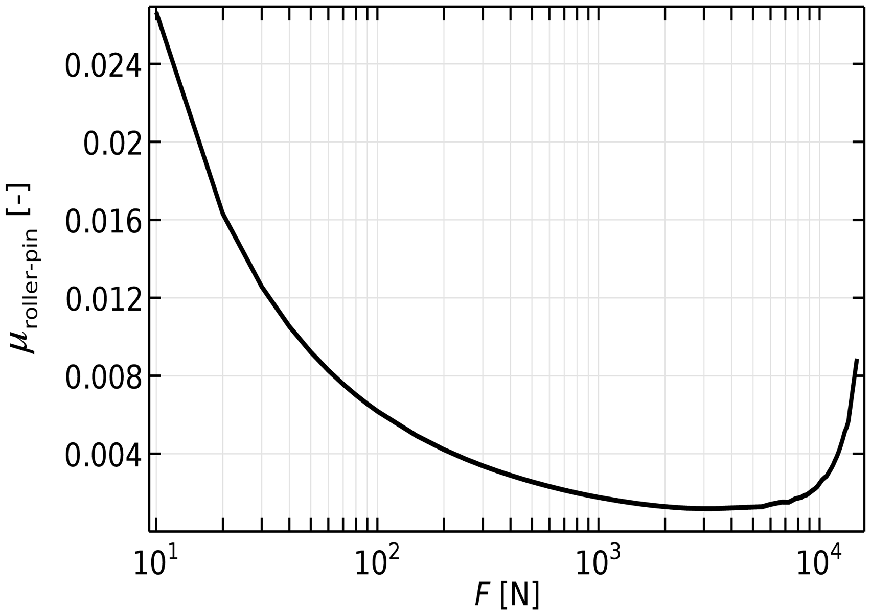

The power losses corresponding to cam–roller and roller–pin contact are shown in Figure 14. As reported in earlier work Alakhramsing et al., ⁶ rolling friction losses play a dominant role as roller slip appears to be negligible. Also note that the rolling power losses are proportional to the sum velocity and almost independent of contact force. This is also why the total power losses for the cam–roller contact cycles are around 6 W with minor variations.

Figure 14.

Evolution of the individual power losses, corresponding to the cam–roller and roller–pin contact, as a function of cam angle θ.

Figure 15.

Evolution of friction coefficients 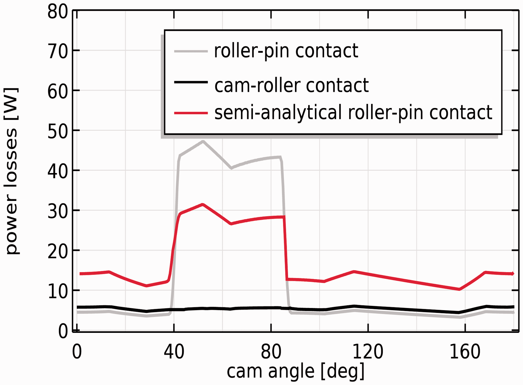${\mu }_{\text{cam}-\text{roller}}$ and ${\mu }_{\text{roller}-\text{pin}}$ as a function of cam angle θ.

The power losses for the roller–pin contact, obtained using the full transient analysis, are compared with those obtained using the rigid semianalytical model as used by Alakhramsing et al. ⁶ For the roller–pin contact, which is a sliding contact, the power losses are proportional to the sliding speed. In the base circle regions the semianalytical model, which does not include elastic deformation, overestimates the power losses as the contact area is overestimated and the film thickness is underestimated. Furthermore, in the nose region the semianalytical model underestimates the power losses as the semianalytical model assumes isoviscous behavior, i.e. the viscosity increases significantly in the cam’s nose region.

Conclusions

A multyphysics model, enabling coupled transient EHL simulations of cam–roller and roller–pin contact in cam–roller follower mechanisms, has been developed. For the transient analysis a heavily loaded cam–roller follower unit, as part of a heavy-duty diesel engine, was considered.

It has been shown that likewise the cam–roller contact, the roller–pin contact also inhibits typical finite line contact EHL characteristics at high loads. Coming on to the nature of finite line contacts, the importance of axial profiling for the roller–pin contact is highlighted here as edge loading is reduced.

Another important contribution made in this work is that it has been shown that elastic deformation of roller and pin significantly enhances the film thickness distribution in the roller–pin contact. Also, prediction of other crucial performance indicators such as maximum pressure and power losses has significantly improved when compared to the models assuming rigid surfaces.

Finally, for heavily loaded cam–roller followers, as studied in this work, it can be concluded that: (i) transient effects are negligible and quasi-static analysis yields sufficiently accurate results, (ii) roller slip is negligible due to high contact forces and pure rolling may be assumed, (iii) highest power losses are associated with the roller–pin contact due to simple sliding and relatively larger contact area as compared to the cam–roller contact and, (iv) due to the nontypical EHL characteristics of both cam–roller and roller–pin contact numerical analysis becomes inevitable for evaluation of crucial tribological performance indicators.

Due to the finite line contact nature of the roller–pin contact axial surface profiling seems to be a promising way to optimize the tribological performance of this contact. Extension of the model to other features, such as mixed lubrication, non-Newtonian, and optimizing routines, is suggested for future work.