Lubrication and frictional analysis of cam–roller follower mechanisms

Abstract

In this work, a full numerical solution to the cam–roller follower-lubricated contact is provided. The general framework of this model is based on a model describing the kinematics, a finite length line contact isothermal-EHL model for the cam–roller contact and a semi-analytical lubrication model for the roller–pin bearing. These models are interlinked via an improved roller–pin friction model. For the numerical study, a cam–roller follower pair, as part of the fuel injection system in Diesel engines, was analyzed. The results, including the evolution of power losses, minimum film thickness and maximum pressures, are compared with analytical solutions corresponding to infinite line contact models. The main findings of this work are that for accurate prediction of crucial performance indicators such as minimum film thickness, maximum pressure and power losses a finite length line contact analysis is necessary due to non-typical EHL characteristics of the pressure and film thickness distributions. Furthermore, due to the high contact forces associated with cam–roller pairs as part of fuel injection units, rolling friction is the dominant power loss contributor as roller slippage appears to be negligible. Finally, the influence of the different roller axial surface profiles on minimum film thickness, maximum pressure and power loss is shown to be significant. In fact, due to larger contact area, the maximum pressure can be reduced and the minimum film thickness can be increased significantly, however, at the cost of higher power losses.

Introduction

The design of the injection cams in heavy-duty diesel engines is from a tribological perspective one the most challenging technical tasks as these components are subjected to instantaneous heavily loaded pressures from the fuel injector. Lubrication is of significant importance to reduce friction and wear. Apart from the high fluctuating loads, varying radius of curvature and lubricant entrainment speed make the tribological design even more challenging.

The preference of roller followers over sliding followers is more often made by engine manufactures due to reduced friction losses and occurrence of wear. ¹ As reported by Lee and Patterson, ² the problem of wear on the interacting surfaces still remains if slip occurs. Furthermore, accurate estimation of friction losses depends to a large extend on the sliding velocity. In contrast to a cam and sliding follower, the slide-to-roll ratio (SRR) for the cam and roller follower is additionally also dependent on the lubricant rheology and friction at the roller–pin interface. Most previous studies assumed pure rolling conditions,^3–5 i.e. the cam and roller surface speed are assumed to be equal. One may only find a few published studies on the lubrication analysis of the cam and roller follower contact that considers the possibility of roller slippage along the cam surface. Chiu ⁶ and later Ji and Taylor ⁷ developed a theoretical roller friction model from which they concluded that slippage exists, especially at high cam rotational speeds due to large inertia forces. The occurrence of roller slippage has also been proven experimentally. ⁸

Axial surface profiling of the rollers is often utilized to minimize stress concentrations that are generated at the extremities of the contact. It has been proven both theoretically and experimentally that the maximum pressure and minimum film thickness occur near the regions where axial profiling starts.^9–11 Disregarding axial surface profiling, as assumed in traditional infinite line contact models, may lead to inaccurate estimation of crucial lubrication performance indicators such as the minimum film thickness and maximum pressure. Consequently, frictional losses may also deviate significantly from reality as these are dependent on the film thickness and pressure distribution.

Finite line contact models would therefore be more appropriate to describe the EHL behavior of the contact. Finite line contact problems of cam and flat-faced follower conjunctions have been studied in the past.^12,13 Shirzadegan et al. ¹⁴ studied the finite line contact problem of a cam–roller follower. However, roller slippage was disregarded in their analysis and no results concerning the working frictional losses at the lubricated interfaces were presented. Turtorro et al. ¹⁵ also presented a cam–roller lubrication model which allows for roller slippage; however, their solution for the lubricant film thickness is obtained using analytical expressions rather than solving the Reynolds equations.

From the previously mentioned studies, it may be concluded that up till date, a limited number of studies concerning the lubrication analysis of cam–roller followers based on a full numerical solution, i.e. taking into account non-typical EHL characteristics of the finite length line contact and possible roller slippage, have been presented. However, the approach followed in the aforementioned studies can be applied to perform more in-depth investigations into the frictional behavior of cam–roller follower mechanisms.

Therefore, in this paper, an FEM-based lubrication model, applicable to any cam–roller follower system, is developed. In the present study, we assume that thermal effects are insignificant, and therefore isothermal conditions are assumed. The finite line contact EHL model is similar to the one presented in Shirzadegan et al., ¹⁴ which efficiently takes care of roller axial surface profiling. An improved roller friction model, to determine roller slippage, is presented. In contrast to previous models, the presented roller friction model also takes into account the film thickness distribution in the roller–pin bearing. For the numerical analysis, a cam–roller follower unit as part of the fuel injection equipment of a diesel engine was considered. The results analyzed, are the evolution of the minimum film thickness, maximum pressure, individual frictional losses and roller slippage along the cam surface. Furthermore, the influence of different roller axial surface profiles on the aforementioned variables is analyzed.

Mathematical model

The type of configuration considered in this work is that of a cam and reciprocating roller follower, in which the roller is free to rotate due to traction enforced by the cam. The roller is supported by a “low-friction” hydrodynamic bearing. The considered configuration, with an emphasis on the working frictional forces at the lubricated interfaces, is presented in Figure 1. The lubricated interfaces in the configuration are separately defined as cam–roller interface and roller–pin interface for the sake of distinctness.

Figure 1.

Cam and roller follower configuration with an emphasis on frictional forces acting at the cam–roller and roller–pin interface.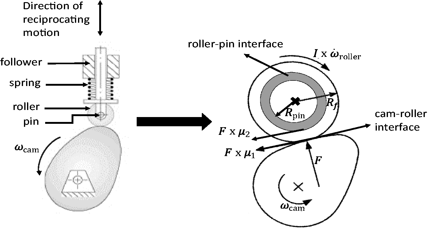

In the first part of this section, a kinematic analysis for the considered configuration is presented. The kinematic analysis provides input, in terms of reduced radius of curvature, entrainment velocity and normal contact force variations that enters the EHL calculations. The second part presents the governing EHL equations to describe the tribological behavior in the cam–roller contact. The third part provides details concerning the individual evaluation of frictional losses, due to hydrodynamic rolling and sliding at cam–roller and roller–pin interfaces. Finally, the last part of this section treats the roller slippage calculation.

Kinematic analysis

The kinematic model adopted in this work stems from Matthews and Sadeghi ⁴ who developed a general procedure to derive the variations in reduced radius of curvature and entrainment velocity for several types of cam–follower configurations. For this reason, only the main equations are presented, and for details the reader is referred to Matthews and Sadeghi. ⁴ Figure 2 shows the cam and reciprocating follower configuration along with nomenclature, coordinate system and angles. The kinematic analysis of the cam and reciprocating roller follower mechanism requires the lift curve $l(\theta )$ , outer radius of roller R_f and global position of cam and follower as input. Note that subscripts “f” and “fc” denote follower and follower center, respectively. The lift curve $l(\theta )$ illustrates the vertical displacement of the roller follower center as depicted in Figure 2.

Figure 2.

Cam and roller follower configuration with specification of coordinate system and nomenclature.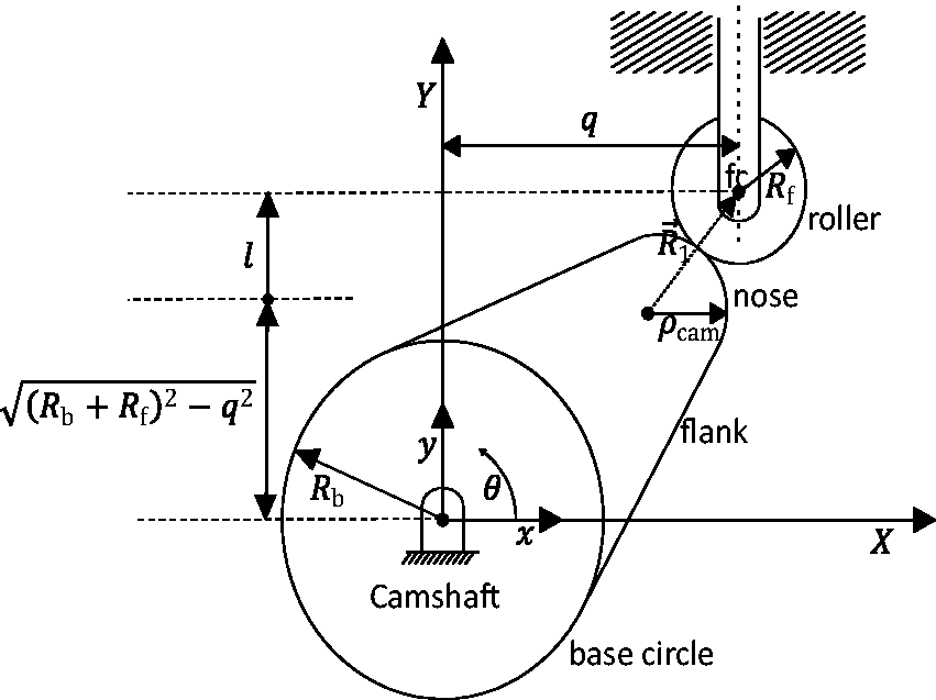

With global position, (X, Y) is meant the center position of cam and follower in a coordinate system where the origin is fixed to the ground. However, commonly a relative coordinate system (x, y), where the coordinate system is fixed to the camshaft, is used to derive the instantaneous radius of curvature. Transformation from the global coordinate system to the relative coordinate system, or vice versa, can be made using

$$[xy]=[\cos \theta \sin \theta -\sin \theta \cos \theta ][XY]$$

(1a)

$$[XY]=[\cos \theta -\sin \theta \sin \theta \cos \theta ][xy]$$

(1b)

Note that angles are measured positive in counterclockwise direction. As mentioned earlier, the lift curve $l(\theta )$ is needed as input for derivation. ¹ The lift curve $l(\theta )$ and fuel pressure $P_{\text{fuel}}(\theta )$ profile are specified in n data points. These data points are (usually) measured values with increments of a specified angle (usually less than one degree cam angle). The smaller this increment the higher the resolution of the profile and hence the accuracy of solution. The n data points are spline-interpolated with respect to cam angle, i.e. the discrete displacement profile is interpolated to obtain a third-order piecewise continuous polynomial fit for displacement versus cam angle. The derivatives of this polynomial fit will give the velocity and acceleration profiles. A similar procedure was applied to deduce the contact force profile of the kinematic variations. In the equations presented hereafter, the angle $(\theta )$ after the dependent variables are omitted for the sake of brevity.

The global coordinates of the roller follower center ( $X_{\text{fc}},Y_{\text{fc}}$ ) are given as

$$\{X_{\text{fc}}=q{Y}_{\text{fc}}=\sqrt{(R_{\text{b}}+R_{\text{f}}{)}^2-q^2}+l$$

(2) where $R_{\text{b}}$ is the base circle radius and q is the horizontal offset of reciprocating follower.

Calculation of cam radius of curvature

From mathematics, we know that the radius of curvature ρ at a certain point, that moves along a path in the relative frame (x, y), can be computed as follows

$$\rho =\frac{f^3}{f_y{f}_x\text{'}-f_x{f}_y\text{'}}$$

(3) where the kinematic coefficients f, f_x, f_y, $f_x\text{'}$ and $f_y\text{'}$ are calculated as follows

$$\{f_x=\frac{\text{d}x}{\text{d}\theta }=\frac{\text{d}X}{\text{d}\theta }\cos \theta -X\sin \theta +\frac{\text{d}Y}{\text{d}\theta }\sin \theta +Y\cos \theta f_y=\frac{\text{d}y}{\text{d}\theta }=-\frac{\text{d}X}{\text{d}\theta }\sin \theta -X\cos \theta +\frac{\text{d}Y}{\text{d}\theta }\cos \theta -Y\sin \theta f_x\text{'}=\frac{{\text{d}}^{2}x}{\text{d}{\theta }^2}=\frac{{\text{d}}^{2}X}{\text{d}{\theta }^2}\cos \theta +\frac{{\text{d}}^{2}Y}{\text{d}{\theta }^2}\sin \theta -2\frac{\text{d}X}{\text{d}\theta }\sin \theta +2\frac{\text{d}Y}{\text{d}\theta }\cos \theta -X\cos \theta -Y\sin \theta f_y\text{'}=\frac{{\text{d}}^{2}y}{\text{d}{\theta }^2}=-\frac{{\text{d}}^{2}X}{\text{d}{\theta }^2}\sin \theta +\frac{{\text{d}}^{2}Y}{\text{d}{\theta }^2}\cos \theta -2\frac{\text{d}X}{\text{d}\theta }\cos \theta -2\frac{\text{d}Y}{\text{d}\theta }\sin \theta +X\sin \theta -Y\cos \theta f=\sqrt{f_x^2+f_y^2}$$

(4)

Now, by substituting the expressions for the roller follower center (equation (2)) for the above-defined kinematic coefficients, and then again substituting in the expression for calculation of the radius of curvature, equation (3) gives the instantaneous cam radius of curvature

$${\rho }_{\text{cam}}=\frac{f_{\text{fc}}^3}{f_{y,\text{fc}}{f}_{x,\text{fc}}\text{'}-f_{x,\text{fc}}{f}_{y,\text{fc}}\text{'}}-R_f$$

(5)

The equivalent radius of curvature R_x that enters the EHL calculations is then calculated as follows

$$R_x=(\frac{1}{{\rho }_{\text{cam}}}+\frac{1}{R_{\text{f}}}{)}^{-1}$$

(6)

Calculation of cam surface velocity

The mean entraining velocity of lubricant that enters the EHL calculations is calculated as follows

$$U_{\text{m}}=\frac{U_{\text{cam}}+U_{\text{roller}}}{2}$$

(7) where the surface velocities of cam $U_{\text{cam}}$ needs to be evaluated from the kinematic analysis and is dependent on the cam radius of curvature ${\rho }_{\text{cam}}$ and cam rotational speed ${\omega }_{\text{cam}}$ . The roller follower surface velocity $U_{\text{roller}}$ depends on traction caused by the cam. The calculation of $U_{\text{roller}}$ is treated in the next subsection.

Vector ${\overrightarrow{R}}_1$ , in Figure 2, can be interpreted as an imaginary link between the point of contact ( $X_{\text{c}},Y_{\text{c}}$ ) and center of the roller follower ( $X_{\text{fc}},Y_{\text{fc}}$ ). At this point, it is worth noting that vector ${\overrightarrow{R}}_1$ always passes the point of contact, and therefore the point of contact itself has no relative motion to vector ${\overrightarrow{R}}_1$ . Therefore, the velocity of a point on the cam surface, relative to the point of contact is actually equal to the velocity of that same point relative to vector ${\overrightarrow{R}}_1$ . In equation form, this yields

$$U_{\text{cam}}={\rho }_{\text{cam}}{\omega }_{\text{cam}}(1-h_1)$$

(8) where the kinematic coefficient h₁ denotes the variation of the direction of vector ${\overrightarrow{R}}_1$ and is thus computed as follows

$$h_1=\frac{\text{d}{\phi }_1}{\text{d}\theta }$$

(9) where the direction of vector ${\overrightarrow{R}}_1,{\phi }_1$ , is computed as follows

$${\phi }_1=\tan (\frac{Y_{\text{fc}}-Y_{\text{c}}}{X_{\text{fc}}-X_{\text{c}}}{)}^{-1}$$

(10)

The point of contact ( $x_{\text{c}},y_{\text{c}}$ ), in the relative coordinate system, is given by

$$\{x_{\text{c}}=x_{\text{fc}}+R_f\frac{f_{y,\text{fc}}}{f_{\text{fc}}}{y}_{\text{c}}=y_{\text{fc}}-R_f\frac{f_{x,\text{fc}}}{f_{\text{fc}}}$$

(11) where the relative coordinates ( $x_{\text{fc}},y_{\text{fc}}$ ) are deduced by transforming the global coordinates ( $X_{\text{fc}},Y_{\text{fc}}$ ) according to equation (1a). The global coordinates of the point of contact ( $X_{\text{c}},Y_{\text{c}}$ ) can then be obtained by transforming equation (11) by means of equation (1b).

Similar to equation (8), the roller surface speed can be computed as follows

$$U_{\text{roller}}=-R_f{\omega }_{\text{cam}}(\frac{{\omega }_{\text{roller}}}{{\omega }_{\text{cam}}}-h_1)$$

(12)

The calculation of the angular velocity of the roller ${\omega }_{\text{roller}}$ will be treated later on in this section.

Calculation of normal contact force

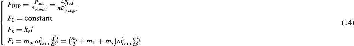
The contact force associated with the cam–follower pair is typically the resultant of inertia forces, caused by moving parts, and the spring force. In the present work, we consider the operating conditions of cam–roller follower pairs in fuel injection pumps (FIP) of heavy-duty diesel engines. These pumps are used to generate high fuel pressures for injection. Therefore, in addition to inertia and spring forces, the injection force acting on the plunger also needs to be considered.

In order to simplify the analysis, a few realistic assumptions are made. These are: (i) the complete tappet including roller, pin, spring, plunger, etc. is considered as a single moving mass, (ii) each individual component is considered as a single lumped mass, (iii) the rotational velocity of the pump is constant and is also not affected by fluctuations of engine strokes, (iv) the moving mass of the spring is assumed to be a third of its mass Zhu and Taylor, ¹⁶ (v) the spring stiffness is linear and finally, (vi) there is no offset and/or eccentricity of the cam to the center of the roller.

With these simplifications, the total acting force is computed as follows

$$F_{\text{total}}=\underset{\text{hydraulicforce}}{\underbrace{F_{\text{FIP}}}}+\underset{\text{pre}-\text{load}}{\underbrace{F_0}}+\underset{\text{springforce}}{\underbrace{F_{\text{s}}}}+\underset{\text{inertiaforce}}{\underbrace{F_{\text{i}}}}$$

(13) where the individual forces are calculated as

$$\{F_{\text{FIP}}=\frac{P_{\text{fuel}}}{A_{\text{plunger}}}=\frac{4P_{\text{fuel}}}{\pi D_{\text{plunger}}^2}{F}_0=\text{constant}{F}_{\text{s}}=k_{\text{s}}l{F}_{\text{i}}=m_{\text{eq}}{\omega }_{\text{cam}}^2\frac{{\text{d}}^{2}l}{\text{d}{\theta }^2}=(\frac{m_{\text{s}}}{3}+m_{\text{T}}+m_{\text{v}}){\omega }_{\text{cam}}^2\frac{{\text{d}}^{2}l}{\text{d}{\theta }^2}$$

(14) where $k_{\text{s}},D_{\text{plunger}},m_{\text{s}},m_{\text{T}},m_{\text{v}}$ are the spring stiffness, plunger diameter, spring mass, tappet mass and valve train mass, respectively.

For the cam and roller follower configuration, the pressure angle θ_P is an important design parameter as it limits the steepness of the cam in the design process. The pressure angle is defined as the angle between the direction of axis transmission and direction of motion of the follower. The pressure angle is calculated as follows

$${\theta }_P=\tan (\frac{X_{\text{fc}}-X_{\text{c}}}{Y_{\text{fc}}-Y_{\text{c}}}{)}^{-1}$$

(15)

The actual acting normal contact force, that enters the EHL calculations, is then computed as follows

$$F=F_{\text{total}}\cos {\theta }_P$$

(16)

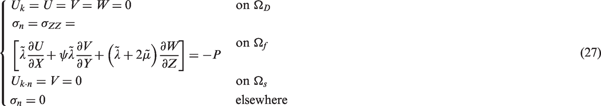
Governing EHL equations for cam–roller contact

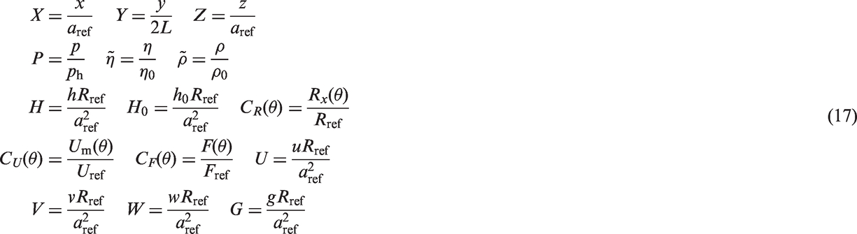
As mentioned earlier, the EHL model here is similar to that presented by Shirzadegan et al. ¹⁴ The model leans on a full-system finite element resolution of the EHL equations. In this work, only the main equations are recalled, and for more details the reader is referred to Shirzadegan et al. ¹⁴ All EHL equations are presented in dimensionless form. Hence, the following (dimensionless) variables and parameters are introduced

$$X=\frac{x}{a_{\text{ref}}}Y=\frac{y}{2L}Z=\frac{z}{a_{\text{ref}}}P=\frac{p}{p_{\text{h}}}\stackrel{\sim }{\eta }=\frac{\eta }{{\eta }_0}\stackrel{\sim }{\rho }=\frac{\rho }{{\rho }_0}H=\frac{{\mathrm{hR}}_{\text{ref}}}{a_{\text{ref}}^2}{H}_0=\frac{h_0{R}_{\text{ref}}}{a_{\text{ref}}^2}{C}_R(\theta )=\frac{R_x(\theta )}{R_{\text{ref}}}{C}_U(\theta )=\frac{U_{\text{m}}(\theta )}{U_{\text{ref}}}{C}_F(\theta )=\frac{F(\theta )}{F_{\text{ref}}}U=\frac{{\mathrm{uR}}_{\text{ref}}}{a_{\text{ref}}^2}V=\frac{{\mathrm{vR}}_{\text{ref}}}{a_{\text{ref}}^2}W=\frac{{\mathrm{wR}}_{\text{ref}}}{a_{\text{ref}}^2}G=\frac{{\mathrm{gR}}_{\text{ref}}}{a_{\text{ref}}^2}$$

(17) with Hertzian parameters defined as follows

$$p_{\text{h}}=\frac{2F_{\text{ref}}}{\pi {\mathrm{La}}_{\text{ref}}}{a}_{\text{ref}}=\sqrt{\frac{8F_{\text{ref}}{R}_{\text{ref}}}{\pi \mathrm{LE}\text{'}}}E\text{'}=\frac{2}{\frac{1-{\nu }_{\text{cam}}^2}{E_{\text{cam}}}+\frac{1-{\nu }_{\text{roller}}^2}{E_{\text{roller}}}}$$

(18) where the subscript “ref” denotes the reference operating conditions. Figure 3 gives the equivalent computational domain for the finite line contact problem. Ω denotes the finite elastic domain for calculation of the displacement fields. The dimensions of 60 × 60 × 2 are chosen in such a way to mimic a half-space for calculation of the elastic displacement field. Boundary Ω _f , with dimensions of $-4.5\le X\le 1.5$ and $-1\le Y\le 1$ , stands for the fluid film domain used to solve for the pressure distribution by means of the Reynolds equation. Finally, Ω _D denotes the bottom boundary of the finite elastic domain.

Figure 3.

Equivalent geometry for EHL analysis of the finite line contact problem. Note that the dimensions are exaggerated for the sake of clarity.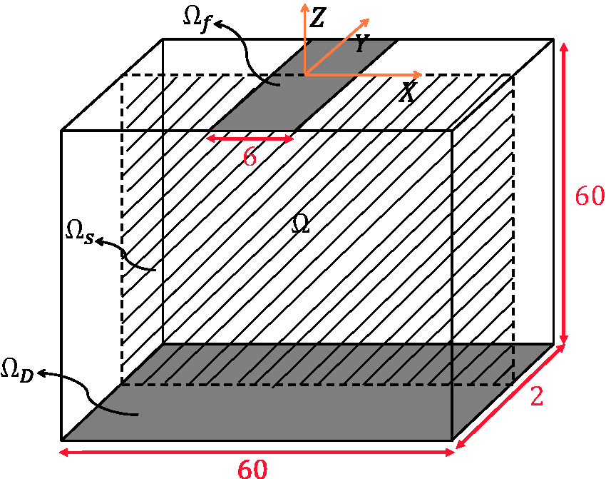

Reynolds equation

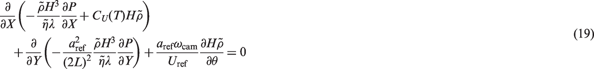
The dimensionless Reynolds equation is written as follows

$$\frac{\partial }{\partial X}(-\frac{\stackrel{\sim }{\rho }{H}^3}{\stackrel{\sim }{\eta }\lambda }\frac{\partial P}{\partial X}+C_U(T)H\stackrel{\sim }{\rho })+\frac{\partial }{\partial Y}(-\frac{a_{\text{ref}}^2}{(2L{)}^2}\frac{\stackrel{\sim }{\rho }{H}^3}{\stackrel{\sim }{\eta }\lambda }\frac{\partial P}{\partial Y})+\frac{a_{\text{ref}}{\omega }_{\text{cam}}}{U_{\text{ref}}}\frac{\partial H\stackrel{\sim }{\rho }}{\partial \theta }=0$$

(19) where $\lambda =\frac{12U_{\text{ref}}{\eta }_0{R}_x^2}{a^3{p}_{\text{h}}}$ is the dimensionless speed parameter, and $\stackrel{\sim }{\rho }$ and $\stackrel{\sim }{\eta }$ are the dimensionless density and viscosity, respectively. $C_U(\theta )$ represents the variation of the mean entrainment velocity $U_{\text{m}}$ (see equation (7)). Variation of viscosity and density with pressure are modeled according to the Roelands ¹⁷ and Dowson-Higginson ¹⁸ equations, respectively.

The free boundary cavitation problem, arising at the exit of the lubricated contact, is treated according to the penalty formulation of Wu. ¹⁹ In the latter, an auxiliary/penalty term is added to the Reynolds equation to force all negative pressure to zero. It should be mentioned that this term has no influence on regions where $P\ge 0$ and thus consistency of equation (19) is preserved. Wu ¹⁹ also showed that the so-called Reynolds boundary conditions, i.e. $\nabla P·{\overrightarrow{n}}_c=0$ on the cavitation boundary, are automatically satisfied with this approach. ${\overrightarrow{n}}_c$ is the outlet normal vector to the cavitation boundary.

A combination of non-residual and residual-based “artificial diffusion” terms, as detailed in Habchi et al., ²⁰ was added to the weak formulation of equation (19) in order to stabilize the solution at high loads.

Finally, it is assumed that the inlet of the contact is fully flooded and the surface roughness is small enough to be disregarded (smooth surfaces are assumed).

Film thickness expression

The film thickness expression H for a general finite line contact problem may be written as follows

$$H(X,Y,\theta )=H_0(\theta )+\frac{X^2}{2C_R(\theta )}+G(Y,\theta )-W(X,Y,\theta )$$

(20) where H₀ is the rigid body displacement and W is the contribution due to elastic deformation. $C_R(\theta )$ denotes the dimensionless variation of the reduced radius of curvature R_x (see equation (6)). $G(Y,\theta )$ can be any function to approximate the dimensionless geometrical variation of the axial surface profile. Numerical studies in the past, aiming to reduce edge effects due to the finite length, showed that the most favorable effect with respect to edge stress concentration reduction is obtained when the generatrix of the finite line contact corresponds to a logarithmic function. In the present study, the logarithmic expression, as proposed by Fujiwara and Kawase, ²¹ is adopted and is written as follows

$$g(y,\theta )=-A\ln \{1-[1-\text{exp}(\frac{-z_{\text{m}}}{A})](\frac{2y-L_{\text{s}}}{L-L_{\text{s}}}{)}^2\}$$

(21)

Equation (21) corresponds to Figure 4 in which A represents the degree of crowning curvature, $z_{\text{m}}$ is the crown drop at the extremities and $L_{\text{s}}$ is the straight roller length. These three parameters provide more flexibility in roller design. Note also that $g(y,\theta )$ is only valid for $\frac{L_{\text{s}}}{2}\le y\le \frac{L}{2}$ , otherwise zero.

Figure 4.

Roller axial profiling utilizing a logarithmic shape with defined design parameters straight length 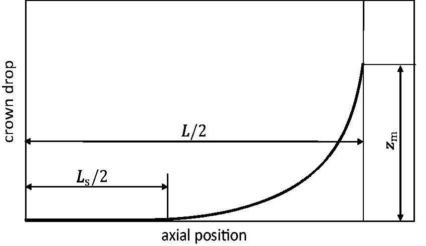$L_{\text{s}}$ , crown drop $z_{\text{m}}$ and crowning curvature A.

Load balance

H₀ is obtained by satisfying the conservation law that states that the applied load should be balanced by the hydrodynamically generated force. In equation form, this can be written as follows

$${\int }_{{\Omega }_f}P(X,Y,\theta )\text{d}\Omega =\pi C_F(\theta )$$

(22) where ${\Omega }_f$ denotes the fluid film domain (see Figure 3) and $C_F(\theta )$ stands for the dimensionless variation of contact force F (see equation (16)). Finally, if symmetry is used (with symmetrical plane ${\Omega }_{\text{s}}$ ), the dimensionless pressure P should be multiplied by a factor of 2.

Calculation of elastic deformation

For the elastic deformation calculation, we make use of the equivalent elasticity property as described in Habchi et al., ²⁰ i.e. two contacting material properties $(E_1,{\nu }_1)$ and $(E_2,{\nu }_2)$ can be reduced to a single component with equivalent material properties $(E_{\text{eq}},{\nu }_{\text{eq}})$ . In fact, the (dimensionless) equivalent material properties are calculated as follows ²⁰

$${\stackrel{\sim }{E}}_{\text{eq}}=\frac{E_1^2{E}_2(1+{\nu }_2{)}^2+E_2^2{E}_1(1+{\nu }_1{)}^2}{[E_1(1+{\nu }_2)+E_2(1+{\nu }_1){]}^2}\frac{a_{\text{ref}}}{R_{\text{ref}}{p}_h}$$

(23a)

$${\nu }_{\text{eq}}=\frac{E_1{\nu }_2(1+{\nu }_2)+E_2{\nu }_1(1+{\nu }_1)}{E_1(1+{\nu }_2)+E_1(1+{\nu }_2)}$$

(23b)

From equation (24), it follows that the dimensionless (equivalent) Lamé’s coefficients $\stackrel{\sim }{\mu }$ and $\stackrel{\sim }{\lambda }$ are, respectively, calculated as follows

$$\stackrel{\sim }{\mu }=\frac{{\stackrel{\sim }{E}}_{\text{eq}}}{2(1+{\nu }_{\text{eq}})}$$

(24a)

$$\stackrel{\sim }{\lambda }=\frac{{\nu }_{\text{eq}}{\stackrel{\sim }{E}}_{\text{eq}}}{(1-2{\nu }_{\text{eq}})(1+{\nu }_{\text{eq}})}$$

(24b) where ( ${\stackrel{\sim }{E}}_{\text{eq}},{\nu }_{\text{eq}}$ ) are calculated by means of equation (23). The 3D-elasticity equations are applied to the dimensionless domain Ω to compute the total elastic deformation. The following system of equations is derived for calculation of the elastic displacement field ¹⁴

$$\frac{\partial }{\partial X}[(\stackrel{\sim }{\lambda }+2\stackrel{\sim }{\mu })\frac{\partial U}{\partial X}+\psi \stackrel{\sim }{\lambda }\frac{\partial V}{\partial Y}+\stackrel{\sim }{\lambda }\frac{\partial W}{\partial Z}]+\psi \frac{\partial }{\partial Y}\times [\stackrel{\sim }{\mu }(\psi \frac{\partial U}{\partial Y}+\frac{\partial V}{\partial X})]+\frac{\partial }{\partial Z}[\stackrel{\sim }{\mu }(\frac{\partial U}{\partial Z}+\frac{\partial W}{\partial X})]=0,\frac{\partial }{\partial X}[\stackrel{\sim }{\mu }(\psi \frac{\partial U}{\partial Y}+\frac{\partial V}{\partial X})]+\psi \frac{\partial }{\partial Y}[\stackrel{\sim }{\lambda }\frac{\partial U}{\partial X}+\psi (\stackrel{\sim }{\lambda }+2\stackrel{\sim }{\mu })\frac{\partial V}{\partial Y}+\stackrel{\sim }{\lambda }\frac{\partial W}{\partial Z}]+\frac{\partial }{\partial Z}[\stackrel{\sim }{\mu }(\frac{\partial V}{\partial Z}+\psi \frac{\partial W}{\partial Y})]=0,\frac{\partial }{\partial X}[\stackrel{\sim }{\mu }(\frac{\partial U}{\partial Z}+\frac{\partial W}{\partial X})]+\psi \frac{\partial }{\partial Y}[\stackrel{\sim }{\mu }(\frac{\partial V}{\partial Z}+\psi \frac{\partial W}{\partial Y})]+\frac{\partial }{\partial Z}[\stackrel{\sim }{\lambda }\frac{\partial U}{\partial X}+\psi \stackrel{\sim }{\lambda }\frac{\partial V}{\partial Y}+(\stackrel{\sim }{\lambda }+2\stackrel{\sim }{\mu })\frac{\partial W}{\partial Z}]=0$$

(25) where $\psi =a_{\text{ref}}/2L$ .

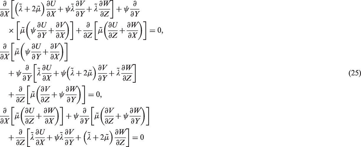
Boundary conditions

In order to obtain a unique solution for the EHL problem, proper boundary conditions (BCs) need to be imposed.

For the Reynolds equation, these are summarized as follows

$$\{P=0\text{on}\partial {\Omega }_f\nabla P·\text{n}=0\text{on}{\Omega }_s$$

(26)

Note that for the present analysis, the advantage of symmetry of the problem (around symmetrical plane Ω _s ) has been taken in order to reduce the computation effort required.

For the elastic model, the BCs are summarized as follows

$$\{U_k=U=V=W=0\text{on}{\Omega }_D{\sigma }_n={\sigma }_{\mathrm{ZZ}}=[\stackrel{\sim }{\lambda }\frac{\partial U}{\partial X}+\psi \stackrel{\sim }{\lambda }\frac{\partial V}{\partial Y}+(\stackrel{\sim }{\lambda }+2\stackrel{\sim }{\mu })\frac{\partial W}{\partial Z}]=-P\text{on}{\Omega }_f{U}_{k·n}=V=0\text{on}{\Omega }_s{\sigma }_n=0\text{elsewhere}$$

(27)

Friction loss evaluation

The three most important friction-related issues in a cam and roller follower configuration, assuming perfectly smooth surfaces, are: (i) occurrence of roller slippage, resulting in high friction, (ii) the EHL rolling friction that becomes increasingly important for lower degrees of slide-to-roll ratios, and (iii) roller–pin bearing friction. The three aforementioned friction contributors are inter-related.

The total frictional force, acting at the cam–roller interface, consists thus of a sliding and rolling component which are calculated as follows

$$F_s=\frac{2L{\eta }_0{R}_{\text{ref}}}{a_{\text{ref}}}{\int }_{{\Omega }_f}\frac{\stackrel{\sim }{\eta }(U_{\text{roller}}-U_{\text{cam}})}{H}\text{d}\Omega$$

(28a)

$$F_r=\frac{2{\mathrm{La}}_{\text{ref}}^2{p}_h}{R_{\text{ref}}}{\int }_{{\Omega }_f}\frac{H}{2}\frac{\partial P}{\partial X}\text{d}\Omega$$

(28b) where F_s and F_r denote the sliding and rolling friction, respectively. Note the direction of the sliding frictional force F_s coincides with the direction of the sliding velocity $(U_{\text{roller}}-U_{\text{cam}})$ . $U_{\text{cam}}$ and $U_{\text{roller}}$ are evaluated according to equations (8) and (12), respectively. The friction coefficient μ₁, acting at the roller outer surface, can thus be computed as follows

$${\mu }_1=\frac{F_{\text{s}}+F_{\text{r}}}{F}$$

(29)

In the present analysis, the roller–pin is modeled as a full film bearing. High pressures are not expected (due to large contact area), and therefore the viscosity–pressure dependence is neglected here. According to Kushwaha and Rahnejat ¹² and Dowson et al., ²² squeeze film effects are important in cases when the lubricant entrainment velocity profile inhibits points of flow reversal. For the both cam–roller and roller–pin contact, this is not the case (see Figure 7). Hence, for the roller–pin contact squeeze film effects are neglected and quasi-static behavior is assumed instead (see Figure 9(a) which justifies this assumption). The film thickness distribution for the roller bearing with a certain eccentricity e from the central position, can be approximated as follows

$$h_{\text{roller}-\text{pin}}=C(1-n\cos \phi )$$

(30) where C is the radial clearance between roller and pin and $n=\frac{e}{C}$ is the dimensionless eccentricity. The angle φ is the circumferential coordinate defined as starting from the minimum film thickness $h_{\text{min},\text{roller}-\text{pin}}$ of the roller–pin bearing (see Figure 5).

Figure 5.

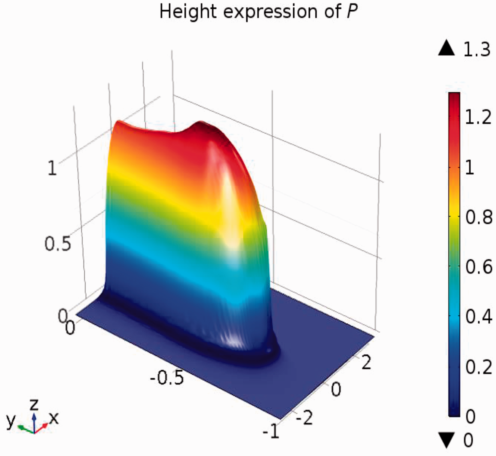
Schematic view of a cylindrical journal bearing with fixed coordinate system (x, y) and moving coordinate system (r, t).

Figure 6.

Height expression of pressure distribution for roller with logarithmic axial profile, viewed from the rear of the contact. Furthermore, F = 7 kN, $U_{\text{m}}=4.2$ m/s and $p_{\text{h}}$  = 1.05 GPa. Note that the dimensions of the contact domain are exaggerated here for the sake of clarity.

Figure 7.

Variation of pumping load 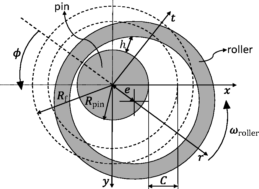$F_{\text{FIP}}$ , lift S and cam surface speed $U_{\text{cam}}$ as function of cam angle θ.

For journal bearings of finite length, the pressure gradients in both directions need to be considered. As such, there is no analytical solution to the Reynolds equation. Several approximate solutions are reported in literature, which are based on asymptotic solutions obtained using the long bearing (Sommerfeld) and short bearing (Ocvirk) solutions. San Andres ²³ derived an approximate analytical solution that gives good results for finite length bearings. This approach gives the following approximate solution for calculating the Sommerfeld number S

$$S=\frac{F}{{\eta }_0{\omega }_{\text{roller}}{\mathrm{LR}}_{\text{pin}}}(\frac{C}{R_{\text{pin}}}{)}^2=\sqrt{{\mathrm{fr}}^2+{\mathrm{ft}}^2}\mathrm{fr}={\mathrm{Zrfr}}_{\infty }{\mathrm{fr}}_{\infty }=\frac{-12n^2}{(2+n^2){\gamma }^2}\mathrm{ft}=\mathrm{Zt}{\mathrm{ft}}_{\infty }{\mathrm{ft}}_{\infty }=\frac{6\pi n}{(2+n^2)\gamma }\mathrm{Zt}=1-\frac{\tanh (\lambda \mathrm{tL}/D)}{\lambda \mathrm{tL}/D}\mathrm{Zr}=1-\frac{\tanh (\lambda \mathrm{rL}/D)}{\lambda \mathrm{rL}/D}\lambda t=(\lambda s-\lambda m)e^{-L/D}+\lambda m\lambda r=\sqrt{2}\lambda t\lambda s=\sqrt{\frac{2+n^2}{2{\gamma }^2}}\lambda m=\sqrt{\frac{2(2+n^2)(1+\gamma )}{4{\gamma }^2+4\gamma -\gamma n^2}}\gamma =\sqrt{(1-n^2)}$$

(31) where $D=2R_{\text{pin}}$ is the pin diameter, $\mathrm{fr}=\mathrm{Fr}/C$ and $\mathrm{ft}=\mathrm{Ft}/C$ are the dimensionless radial and tangential fluid film forces, respectively. Zr and Zt are axial correction functions, used to correct for the radial and tangential fluid film forces, respectively. In Figure 5, the moving radial and tangential coordinate system are represented by axes r and t, respectively. These are conveniently defined here as the fluid film reaction forces, given by equation (31), are defined in the moving coordinate system. Note that the radial axis always joins the roller and pin center points.

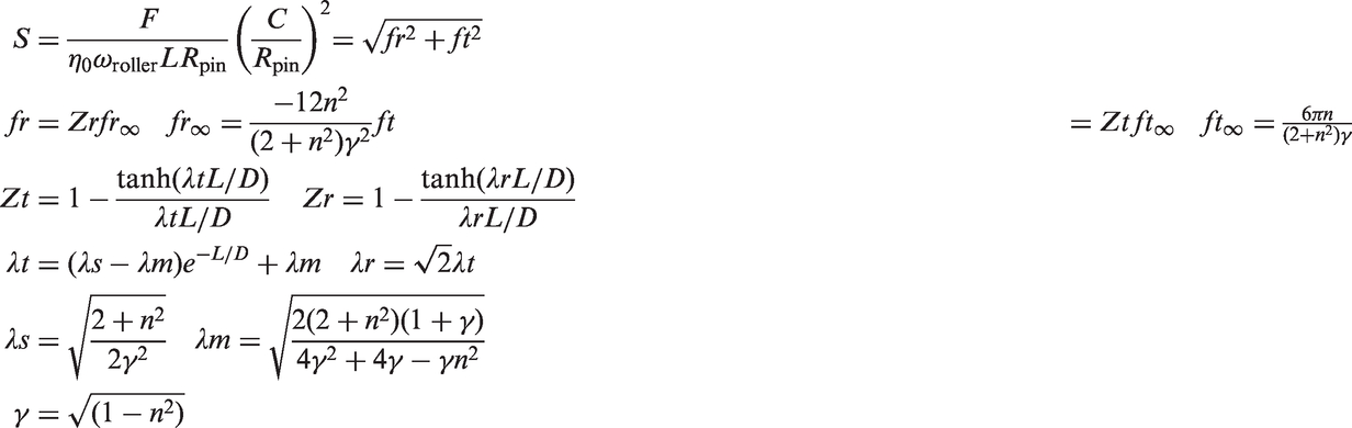
It is worth mentioning that the analytical expressions in equation (31) also take into account the side leakage from the bearing (for more details the reader is asked to refer to San Andres ²³ ).

The bearing friction coefficient μ₂, defined at the roller inner surface, and attitude angle β are calculated as follows ²³

$${\mu }_2=(\frac{2\pi }{S\sqrt{1-n^2}}+\frac{n}{2}\sin (\beta ))(\frac{C}{R})\beta =a\tan (-\mathrm{ft}/\mathrm{fr})$$

(32)

The individual (absolute) instantaneous power losses (in Watts) at the cam–roller and roller–pin contact are respectively computed as follows

$$\text{cam}-\text{rollerslidingpowerloss}=F_s|U_{\text{cam}}-U_{\text{roller}}|$$

(33a)

$$\text{cam}-\text{rollerrollingpowerloss}=F_r|U_{\text{cam}}+U_{\text{roller}}|$$

(33b)

$$\text{roller}-\text{pinpowerloss}={\mu }_2{\mathrm{FR}}_{\text{pin}}{\omega }_{\text{cam}}|\frac{{\omega }_{\text{roller}}}{{\omega }_{\text{cam}}}-h_1|$$

(33c)

The calculation of ${\omega }_{\text{roller}}$ is treated in the next subsection.

Determination of roller slippage

The rotational speed of the roller follower is primarily determined by the driving/tractive torque at the cam–roller interface. Sliding friction acting on the inner wall of the roller resists or tries to slow down the motion of the roller. The roller on itself rotates about its own axis and thus has an angular acceleration. This consequently induces an angular moment of the roller, which is defined as the product of the angular acceleration and mass moment of inertia of the roller.

The roller rotational speed is obtained by balancing the tractive torque (acting at the outer surface of roller) with the combined torques due to roller–pin friction and roller inertia force, by iteratively adjusting the roller rotational speed. In equation form, this yields

$$\underset{\text{tractivetorque}}{\underbrace{{\mu }_1{R}_{f}F}}=\underset{\text{resistingtorque}}{\underbrace{{\mu }_2{R}_{\text{pin}}F}}+\underset{\text{inertiatorque}}{\underbrace{I{\stackrel{·}{\omega }}_{\text{roller}}}}$$

(34) where friction coefficients μ₁ and μ₂ are computed by means of equations (29) and (32), respectively. $I=0.5{\text{m}}_{\text{roller}}(R_{\text{pin}}^2+R_f^2)$ , denotes the mass moment of inertia of the roller. ${\omega }_{\text{roller}}$ is adjusted by means of an iterative procedure to satisfy equation (34).

Note that in this analysis, the frictional torque, due to sliding friction at the end of the roller, has been disregarded as it is assumed that its contribution to the overall resisting torque is small.

From equation (34), it can readily be deduced that if the RHS of the equation is larger than the LHS, it means that the rolling requirement cannot be satisfied and consequently slip will occur. This may be the situation, for example, at higher rotational speeds where inertia forces are high.

Another situation that might increase the possibility of roller slip is when the limiting traction coefficient μ₀, governed by cam–roller lubrication conditions, is exceeded. For full film lubrication, μ₀ is typically governed by the type of lubricant used, mean contact pressure and sum velocity. In this analysis, however, μ₀ is assumed to be constant for the sake of simplicity. If the friction coefficient at the cam–roller interface is found to be larger than μ₀, then maximum friction cannot satisfy the pure rolling condition and roller slip will occur.

Overall numerical procedure

The complete system of equations is formed by the Reynolds equation (19) and elasticity equation (25) with their respective boundary conditions as given by equations (26) and (27), respectively. Additionally, three other equations are added to the complete systems of equations, namely: (i) the load balance equation (22) associated with unknown H₀, (ii) the roller slip equation (34) associated with unknown ${\omega }_{\text{roller}}$ , and (iii) equation (31) to calculate the roller eccentricity associated with unknown n.

The model developed here is solved using the FEM with a multiphysics finite element analysis software COMSOL. ²⁴ The problem is formulated as a set of strongly coupled non-linear partial differential equations. The resulting system of non-linear equations is solved using a monolithic approach where all the dependent variables $P,U,V,W,H_0,{\omega }_{\text{roller}},n$ are collected in one vector of unknowns and simultaneously solved using a Newton-Raphson algorithm. For details concerning the fully coupled numerical procedure, the reader is asked to read Habchi et al. ²⁰ as only the main features are recalled in this work.

A custom tailored mesh, similar to Habchi et al., ²⁰ was employed for the present calculations. For the elastic part, Lagrange quadratic elements were used, while for the hydrodynamic part, Lagrange quintic elements were used. The aforementioned tailored mesh corresponds to approximately 300,000 degrees of freedom.

For steady-state simulations, converged solutions to relative errors ranging between 10⁻³ and 10⁻⁴ are reached within 10 iterations. This corresponds to a computation time of approximately 1.5 minutes on an Intel(R) Core(TM)i7-2600 processor. Realistic initial guesses, as detailed in Shirzadegan et al., ¹⁴ for pressure and H₀ are to be chosen to reduce to the number of iterations required for converged solutions.

For the transient calculations, a steady-state solution was fed as initial guess. Furthermore, a dimensionless time-step $\Delta \theta$ of 0.01 was chosen for the base circle region for the calculations. For remaining regions, where steep kinematic variations occur, a smaller time-step was chosen. The computation time for simulation of the full cam’s lateral surface (360°) is approximately 28 h.

Results

In this section, a comprehensive analysis, for the cam and roller follower, is performed and the results are presented. The configuration parameters and reference operating conditions are given in Table 1.

Table 1.

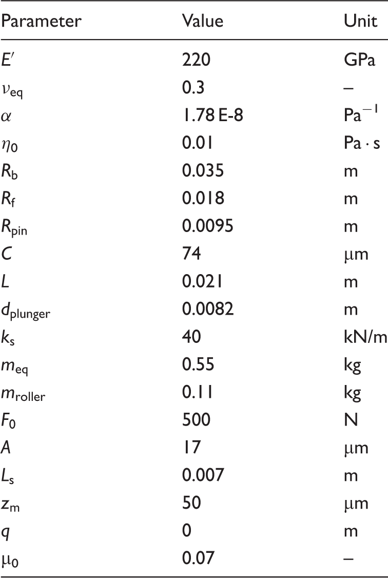
Reference operating conditions and geometrical parameters for cam–roller follower analysis.

Parameter	Value	Unit
$E\text{'}$	220	GPa
${\nu }_{\text{eq}}$	0.3	–
α	1.78 E-8	Pa−1
η 0	0.01	Pa · s
$R_{\text{b}}$	0.035	m
$R_{\text{f}}$	0.018	m
$R_{\text{pin}}$	0.0095	m
C	74	μm
L	0.021	m
$d_{\text{plunger}}$	0.0082	m
$k_{\text{s}}$	40	kN/m
$m_{\text{eq}}$	0.55	kg
$m_{\text{roller}}$	0.11	kg
$F_0$	500	N
A	17	μm
$L_{\text{s}}$	0.007	m
$z_{\text{m}}$	50	μm
q	0	m
μ 0	0.07	–

A height expression of the pressure distribution, for the given reference operating conditions, is shown in Figure 6. Traditional characteristics are observed as for finite line contact solutions, i.e. a secondary pressure peak is observed at the rear of the contact. Near the occurrence of this secondary pressure peak, the absolute minimum film thickness is located (see for instance, Park and Kim ²⁵ ).

Transient analysis

Kinematic variations

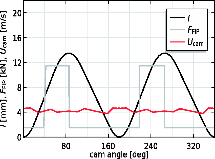
The kinematic variations, such as for contact force, cam surface speed and radius of curvature, are required as an input for the EHL calculations. The kinematic model, as presented earlier, was therefore used to derive profiles for $R_x(\theta ),U_{\text{cam}}(\theta )$ and $F(\theta )$ . In order to derive these profiles, the lift-curve $l(\theta )$ and fuel injection force $F_{\text{FIP}}(\theta )$ are required. Profiles for $l(\theta )$ and $F_{\text{FIP}}(\theta )$ are presented in Figure 7. The derived profile for the cam surface velocity $U_{\text{cam}}(\theta )$ is also provided in the same figure.

Looking at the lift-curve, it can be readily extracted that the considered cam has two lobes/noses, hence two periods of rise and dwell. Furthermore, it is clear that the lift-curve (and hence cam surface speed) and load profile are symmetrical about 180° cam angle.

The profile for the radius of curvature $R_x(\theta )$ can be obtained once $l(\theta )$ is known. The profile for the cam radius of curvature is not shown here; however, the plot for the cam surface velocity is given in Figure 7 for a cam rotational speed of 950 r/min. It can be concluded that the cam surface velocity is fairly constant (with minor variations) over the whole cam’s lateral profile.

The contact force at the cam/roller interface is dominated by the fuel pressure ( $F_{\text{FIP}}$ varies from 1 kN to 12 kN). In fact, a software determines how many grams of fuel are needed per pump stroke, and it activates the pump at a certain cam angle. The pumping action continues till the top of the cam (maximum lift and maximum hydraulic force $F_{\text{FIP},\text{max}}$ ), but once on the top, the pumping motion will go back to zero and the pressure drops. Therefore, the starting angle varies, and the end angle is always at the top of the cam or center of the nose region. The activation and de-activation of the pumping action occur quite abruptly as can be observed from Figure 7.

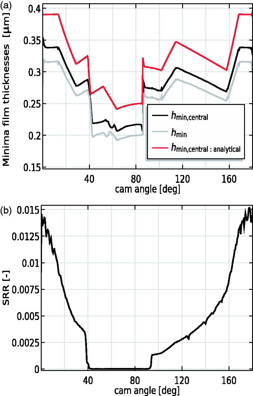
Common rail fuel injection systems are nowadays commonly used. In this system, a common rail, connected to the individual fuel injectors, is utilized in which fuel is kept under constant pressure providing better fuel atomization. In real life, there is a complex mapping of common rail pressure vs. engine rpm and engine torque. A change in common rail pressure will directly influence the pump load. For the present analysis, a worst case scenario was extracted from the complex (software-based) mapping of $F_{\text{FIP}}$ vs. cam speed. This “worst case scenario” mapping corresponds to Figure 8, which depicts the maximum hydraulic force $F_{\text{FIP},\text{max}}$ that can occur at a certain cam speed.

Figure 8.

Mapping of maximum pumping load $F_{\text{FIP},\text{max}}$ against cam rotational speed.

Figure 9.

Evolution of (a) minima film thicknesses and (b) slide-to-roll ratio SRR as function of cam angle. Note the abrupt variations in the overall solution between 40° and 90° cam angle, due to sudden activation of pumping action.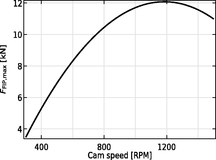

The final contact force profile $F_{\text{total}}(\theta )$ can easily be derived if $l(\theta )$ and $F_{\text{FIP}}(\theta )$ are known, and is not plotted here. It should be stated, however, that the spring and inertia forces appear to be almost negligible compared to the forces arising due to fuel injection pressure.

Results

The results hereafter are presented for cam angle intervals of 0°–180°, as the cam shape is symmetrical about 180° cam angle. In fact, the solution from 0° to 180° is identical to that for 180°–360°. Furthermore, the cam speed is kept fixed at 950 r/min.

The degree of separation between surfaces, defined as specific film thickness, has a very strong influence on the type and amount of wear. Figure 9(a) provides the variation of the absolute and central minimum film thicknesses, $h_{\text{min}}$ and $h_{\text{min},\text{central}}$ , respectively, over the cams lateral surface. Note that $h_{\text{min},\text{central}}$ is the minimum film thickness on the Y = 0 plane, while $h_{\text{min}}$ occurs at the rear of the contact (near the region where axial profiling starts).

Overall, a fairly constant film thickness is predicted as compared to the flat-faced followers due to rolling motion of the follower. The “dips” in the film thickness profile (between 40° and 90°) are due to a rapid increase of the contact force (1 kN to 12 kN), i.e. the contact force remains approximately constant at a value around $F_{\text{FIP},\text{max}}$ , while the cam surface speed also remained constant approximately. The numerically calculated minima film thicknesses are compared against that predicted using the Dowson-Higginson film thickness equation for classical (“infinite”) line contacts. ²⁶ As expected, the analytical solution overestimates $h_{\text{min},\text{central}}$ , as side-leakage is neglected in this approximation. Note that the analytical calculation also assumes “pure rolling conditions”. Assuming a composite surface roughness of 0.2 μm of the opposing surfaces, it can be concluded that the cam/roller contacts operates in the mixed lubrication regime (i.e. $\frac{h_{\text{avg}}}{\sigma }<3$ ).

Comparing the solutions for the analytically and numerically calculated minima film thicknesses, it can also be extracted that transient effects are negligible, i.e. minimum phase lag, due to squeeze-film motion, is observed between the solutions. This observation is in line with previous findings. ¹⁴ Squeeze-film damping is mainly observed for cam–follower configurations in which the lubricant entrainment velocity profile inhibits points of flow reversal, see for instance Dowson et al. ²²

Furthermore, due to large contact forces involved, negligible slippage occurs. It is evident from Figure 9(b) that the SRR remains less than 1.5% over the full cycle. For the present analysis, it was found that the friction coefficient at cam–roller interface μ₁ was less than the limiting traction coefficient μ₀. Therefore, there is a very small difference between $U_{\text{cam}}$ and $U_{\text{roller}}$ . Again, the dips are due to rapid increase in contact force, i.e. the value of SRR is largest at base circle positions where the contact force is lowest. From Figure 9(b), it can also be concluded that the sliding velocity is so small that it is important to include rolling traction when evaluating power losses. For a special case of pure rolling conditions, i.e. $U_{\text{cam}}=U_{\text{roller}}$ , Crecilius et al. ²⁷ developed an analytical expression for the calculation of the hydrodynamic rolling friction. The expression takes into account an exponential dependence of viscosity on pressure and reduces for fully flooded conditions to the following equation

$$F_{r,\text{analytical}}=\frac{4.485{\mathrm{LR}}_x(2{\eta }_0\alpha U_{\text{cam}}/R_x{)}^{0.67}}{2\alpha }$$

(35)

Note that for pure rolling conditions, the sum velocity is $2U_{\text{cam}}$ . Also note that equation (35) consistently agrees with previous findings by Crook ²⁸ in the sense that F_r is proportional with the film thickness (which for EHL is proportional to the sum velocity) and negligibly dependent on the normal contact force. Figure 10(a) presents the individual contributions of rolling and sliding traction on the power losses for the cam–roller interface (refer to equations (33a) and (33b)). As can be extracted from the aforementioned figure, sliding power loss is negligible (almost zero) when compared to rolling power losses, which varies around 5.5 W over the full cam periphery. The analytical solution for rolling power loss (equation (35) multiplied with the sum velocity) is also plotted in the same Figure. As can be observed, the analytical solution overestimates the power loss as this method overestimates the contact area, i.e. for the finite line contact problem, it is known that depending on applied load and axial design parameters the contact area may increase or decrease, while in the analytical approximation, the full axial length of the roller is used as contact area (see equation (35)). It is clear that rolling friction plays an important role in accurate power loss estimations.

Figure 10.

Evolution of individual power losses (due to rolling and sliding friction) for (a) cam–roller interface and (b) roller–pin interface.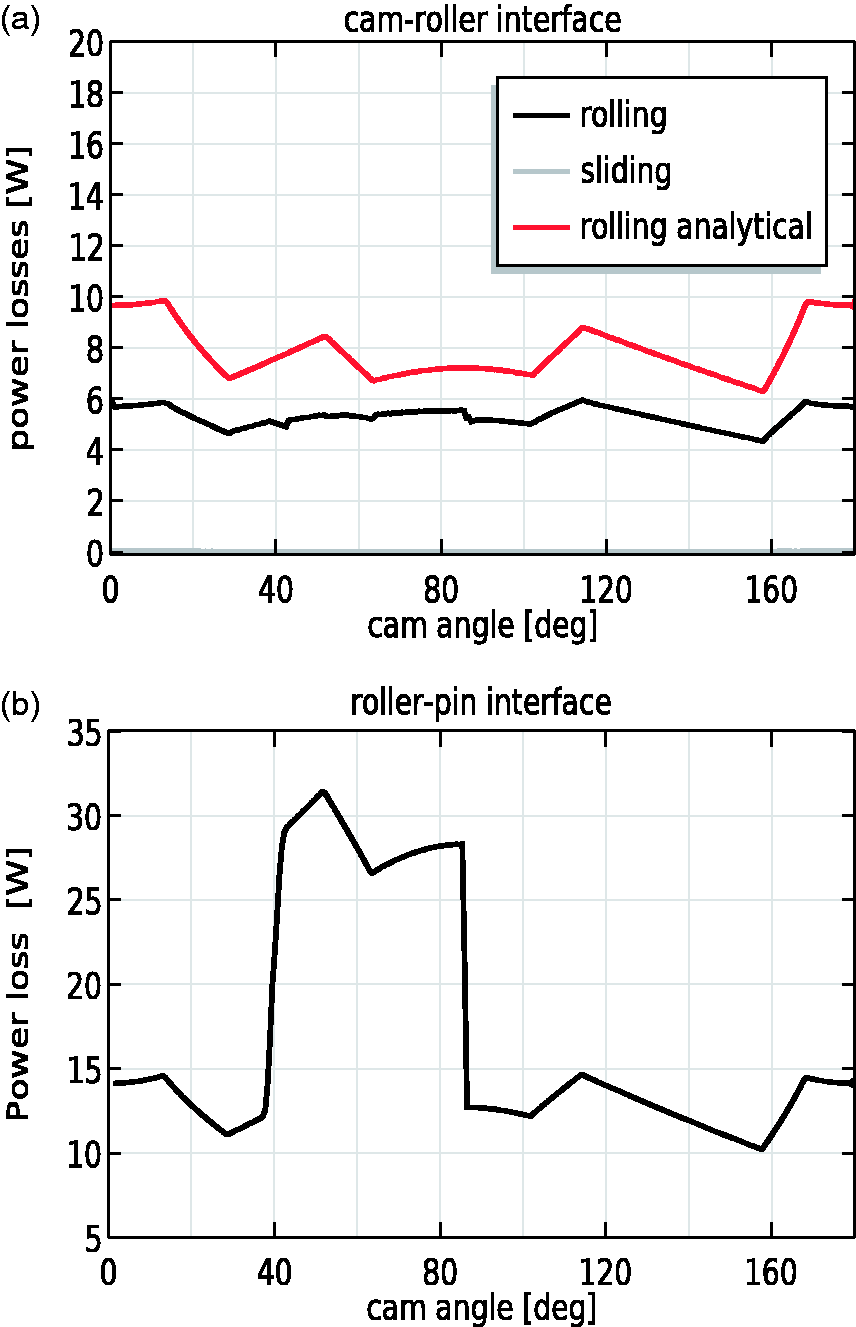

Figure 10(b) plots the evolution of the power loss for the roller–pin interface (refer to equation (33c)). Due to the high contact loads, the total bearing losses reach peak values up to 30 W around the nose region. The sudden rise in frictional losses in the bearing can be attributed to the abrupt variation in contact force. This causes, likewise to cam–roller interface, a “dip” in the minimum film thickness profile of roller–pin bearing (see Figure 11(a)). However, for the roller–pin bearing, this effect is much more amplified as the eccentricity is directly dependent on contact force (see equation (31)).

Figure 11.

Evolution of (a) minimum film thickness for roller–pin interface and (b) maximum pressures for cam–roller interface as a function of cam angle. Note the abrupt variations in the overall solution between 40° and 90° cam angle, due to sudden activation of pumping action.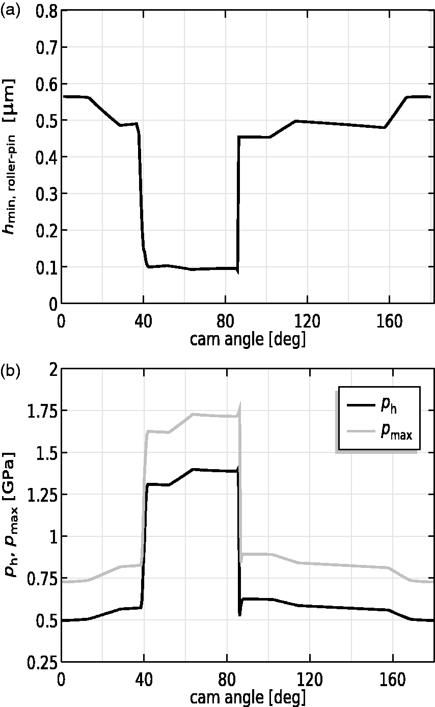

When considering the variation of minimum film thickness at the roller/pin interface, as presented in Figure 11(a), it can be concluded that a poor film thickness of approximately 0.1 μm is predicted around the nose region. This indicates that, assuming a composite roughness of 0.2 μm, the roller–pin bearing operates in mixed or even boundary lubrication regime. The semi-analytical lubrication model for the roller–pin interface does not include deformation of solids which might enhance the film thickness distribution. Furthermore, in this simplistic analysis for the roller–pin interface, it is assumed that surfaces are perfectly smooth, meaning that in the practical case frictional losses will be higher and consequently will induce higher roller slippage. Accurate calculation of the film thickness distribution in the roller–bin bearing is thus extremely important and should be investigated in more detail in future work. The present work, however, certainly emphasizes on the importance of accurate friction calculation in the roller–pin bearing as this contact is equally important as the cam–roller contact, but often weakly included in previous roller friction models.^6,7

Finally, the maximum pressure variation is presented in Figure 11(b). The maximum pressure cycles between 0.5 GPa and 1.8 GPa. The maximum Hertzian pressure $p_{\text{h}}$ for a traditional “infinite” line contact model is also plotted in the same figure. It is clear that the Hertzian analytical solution significantly underestimates the maximum pressure, which for the finite line contact is located near the rear of the contact (secondary pressure peak).

From the aforementioned comparisons between analytical and numerical predictions, it is clear that the usage of traditional analytical tools (applicable to infinite line contacts) may lead to significant deviations from actual solutions. The analytical solutions, however, can be used as a first estimation for preliminary designs. For accurate predictions, numerical studies are inevitable.

Parameter study: Variation of cam rotational speed

It is of interest to analyze the behavior of the minima film thicknesses and other performance indicators over the full range of cam rotational speeds. As earlier mentioned, the maximum fuel injection force is also mapped against cam speed (see Figure 8).

From the results obtained from the transient analysis, presented in the previous section, we could also observe that the worst operating conditions are expected in the nose region of the cam, i.e. power losses, minima film thicknesses and maximum pressures reach their peak values in the nose region. We also saw that the aforementioned performance indicators also remain fairly constant in the nose region because of the contact load that remains almost constant between 40 and 90° cam angle. Therefore, for the parameter study, concerning variation of cam speed, any position in the nose region can be chosen. To be more specific, any position on the nose between the fixed margin of 40 and 90° cam angle can be chosen to examine the variation of crucial tribo-performance indicators.

Figure 12(a) presents the evolution of minima film thicknesses, for cam–roller and roller–pin contact, with increasing cam speed at a fixed cam angle of 68°. For cam–roller contact, it can be seen that the minimum film thickness increases with increasing cam speed even though the contact force on nose region also increases with increasing cam speed. The effect of contact force seems to be less dominant as compared to sum velocity, which is analogously explainable from traditional infinite line contact EHL solutions.

Figure 12.

Variation of crucial design variables such as (a) minima film thicknesses, (b) (inverse) Sommerfeld number (c) maximum pressure and (d and e) power losses with cam rotational speed.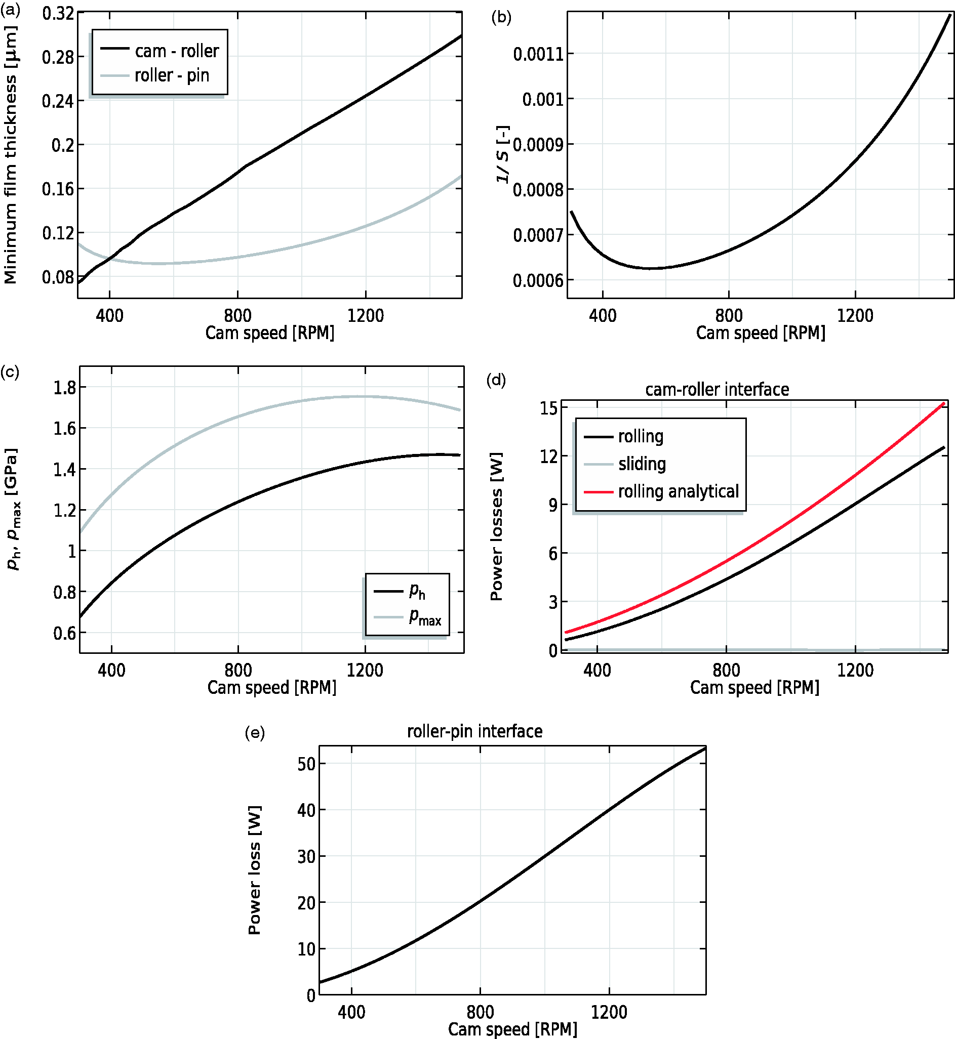

For the roller–pin contact, the minimum film thickness decreases from low to moderate cam speeds and then again increases from moderate to higher cam speeds. This trend can analogously be explained from the variation of the (inverse) Sommerfeld number with increasing cam speeds, which follows the same trend (see Figure 12(b)).

The variation of individual power losses for cam–roller and roller–pin interface is plotted in Figure 12(d) and 12(e), respectively. For the cam–roller interface, we see that the sliding power loss, which is mainly governed by the contact force, remains negligible for the full range of cam speeds, i.e. the contact force increases with cam speed and hence the sliding speed remains minimal. Furthermore, rolling power loss increases with increasing cam speed mainly due to the fact that the sum velocity increases (refer to equation (33b)), and hence, the film thickness increases. The analytical method overestimates the rolling power loss due to overestimation of contact area. For the roller–pin interface, an increase power loss is observed with increase in cam speed. This increase is mainly due to the fact that the sliding speed increases, and hence, viscous shear in this contact increases accordingly.

Finally, an increase in maximum pressure is observed with increasing cam speed (see Figure 12(c)). This is mainly due to the mapping of $F_{\text{FIP},\text{max}}$ against cam speed (see Figure 8). It is no surprise that the maximum pressure will behave similarly as $F_{\text{FIP},\text{max}}$ . Also note that the analytical approximation using the Hertzian theory for line contacts underestimates the maximum pressure over the full range of cam rotational speeds.

Influence of different axial surface profiles

From the results obtained from the transient analysis, it can be extracted that for the considered cam–roller configuration, any position on the nose between the fixed margins of 40°–90° cam angle can be chosen to examine the variation of crucial tribo-performance indicators. It would be of interest to study the effect of different axial profile designs on crucial cam–roller contact performance indicators, such as minimum film thickness, maximum pressure and rolling power loss. The axial profile can be optimized for a certain operating point, to obtain a more uniform axial pressure distribution. Note that for the considered operating conditions, roller slippage around nose region was found to be negligible. Also note that the choice of different roller axial shapes does not influence the results from the semi-analytical lubrication model for the roller–pin contact, as the film thickness is directly correlated with the applied load.

For the present study, three different roller axial surface logarithmic profiles are considered. Table 2 presents the design parameters corresponding to the three different logarithmic profiles (see Figure 13(a)). Note that design 1 is similar to that (given in Table 1) used for the cam–roller analysis. For the present study, the cam angle was fixed at 68°.

Table 2.

Considered logarithmic axial surface profiles.

	$L_{\text{s}}$ (mm)	A (μm)	$z_{\text{m}}$ (μm)
Design 1	7	17	50
Design 2	4	100	100
Design 3	11	10	10

Figure 13.

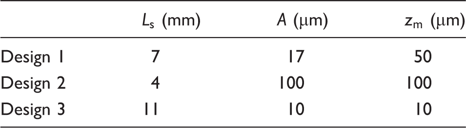
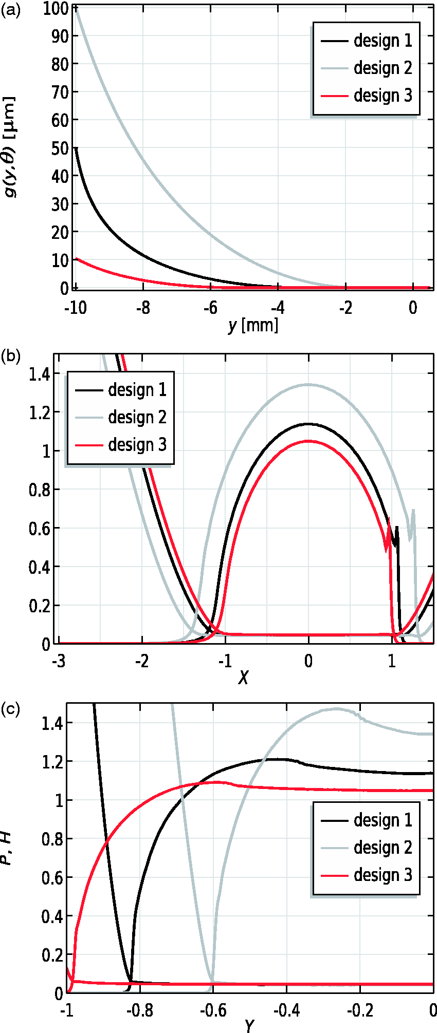
Influence of (a) considered roller axial surface profiles on (b) streamline and (c) axial pressure and film thickness distributions.

Figure 13(b) and 13(c) presents the dimensionless pressure and film thickness distributions along the lines Y = 0 and X = 0, respectively. It can readily be extracted that the most uniform pressure distribution is obtained for design 3. In fact, for design 3, the transverse lubricant flow experiences significantly less geometric discontinuity near the region where axial profiles starts. Consequently, the pressure profile inhibits less steep gradients at the rear of the contact, and thus covers more area to carry the applied load. For this reason, the minimum film thickness increases and maximum pressure decreases when compared to reference design 1 (see Table 3). However, due tot the fact that the covered contact area increases, the power losses also increase for design 3.

Table 3.

Influence of considered axial surface profile design on crucial performance indicators around nose region.

	$h_{\text{min}}$ (μm)	$p_{\text{max}}$ (GPa)	Power loss (W)
Design 1	0.202	1.68	5.75
Design 2	0.175	2.01	4.37
Design 3	0.211	1.51	7.10

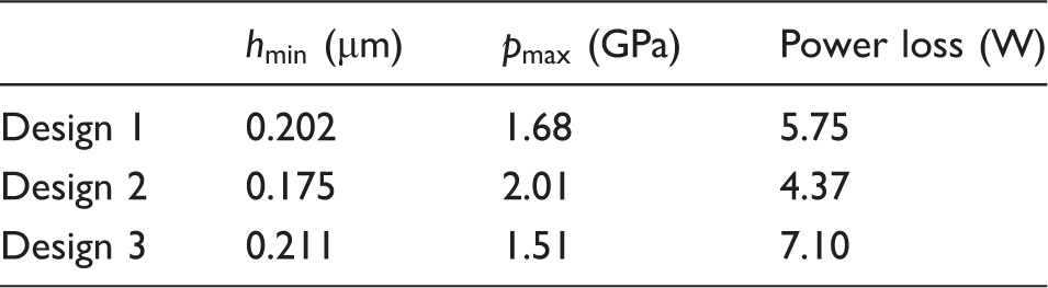
Exact the opposite is observed for design 2, i.e. due to larger geometric discontinuity, the maximum pressure increases and minimum film thickness decreases. However, due to decrease in covered contact area, the power loss decreases. It is clear from the case studies that maximum pressure and minimum film thickness values are improved at the cost higher power losses.

Conclusions

A finite line contact EHL model was utilized to analyze cam–roller follower lubrication conditions. A detailed kinematic analysis was presented to derive variations of load, speed, and radius of curvature with respect to cam angle. The model includes an improved (semi-analytical) roller friction model, which takes into account the roller–pin film thickness distribution. Therefore, friction losses are more accurately estimated, and consequently, the roller slippage prediction is also improved.

For the numerical analysis, a cam and logarithmically profiled roller follower were simulated. The cam–follower pair was assumed to be part of the fuel injection equipment in heavy-duty diesel engines.

It was found that friction losses in the roller–pin contact are highest due to high contact forces (and thus low film thickness) and sliding speeds. The importance of more accurate friction models for the roller–pin contact is highlighted here as this the contact associated with highest power losses and lowest minimum film thickness.

For the cam–roller contact, it can be concluded that rolling friction is the most important power loss contributor as roller slippage was found to be negligible for the load range considered. The results in terms of friction losses, minimum film thickness, and maximum pressure were compared with quasi-statistic analytical solutions corresponding to infinite line contact models. The importance of considering a finite line contact model, instead of an infinite line contact, was clearly emphasized, i.e. traditional line contact model significantly underestimates the maximum pressure and overestimates the minimum film thickness. Also, power loss estimation using the analytical approach may deviate significantly when compared with actual power losses due to overestimation of contact area.

An important observation that was made is that transient effects are negligible; therefore, the quasi-static analysis should also suffice to study the lubrication conditions for the cam–roller pair.

Different roller axial profiles were considered to study their influence on crucial performance indicators around the nose region. It was found that maximum pressure and minimum film thickness values can be improved significantly, however, at the cost of higher power losses. Therefore, suitable optimization routines need to be utilized in order to reach an optimum combination between friction losses, maximum pressure, and minimum film thickness.

Computational times for simulating cam–roller follower lubrication, with usage of the current model, are found to be reasonable. Moreover, the developed model demonstrated the ability to cope with abrupt changes in operating conditions in which the load suddenly increases and decreases. Therefore, this model can certainly be used to study the influence of modifications in cam and/or roller shape design, on the overall efficiency of the cam–follower unit.

The present study focuses on lubrication conditions in a highly loaded cam–roller follower pair in which sliding is found to be insignificant. However, for example, in lightly to moderately loaded cam–roller contacts, where relatively high sliding speeds might occur, extension of the model to non-Newtonian and thermal effects might be important. Also, more extensive rheological formulations^29,30 should then be used. The aforementioned aspects are suggested for future work.