The influence of stick–slip transitions in mixed-friction predictions of heavily loaded cam–roller contacts

Abstract

A load-sharing-based mixed lubrication model, applicable to cam–roller contacts, is developed. Roller slippage is taken into account by means of a roller friction model. Roughness effects in the dry asperity contact component of the mixed lubrication model are taken into account by measuring the real surface topography. The proportion of normal and tangential load due to asperity interaction is obtained from a dry contact stick–slip solver. Lubrication conditions in a cam–roller follower unit, as part of the fuel injection equipment in a heavy-duty diesel engine, are analyzed. Main findings are that stick–slip transitions (or variable asperity contact friction coefficient) are of crucial importance in regions of the cam where the acting contact forces are very high. The contact forces are directly related to the sliding velocity/roller slippage at the cam–roller contact and thus also to the static friction mechanism of asperity interactions. Assuming a constant asperity contact friction coefficient (or assuming that gross sliding has already occurred) in highly loaded regions may lead to large overestimation in the minimal required cam–roller contact friction coefficient in order to keep the roller rolling. The importance of including stick–slip transitions into the mixed lubrication model for the cam–roller contact is amplified with decreasing cam rotational velocity.

Introduction

The cam–roller follower unit as part of the fuel injection equipment in heavy-duty diesel engines is subjected to very high loads coming from the fuel injector. The pressures experienced by cam–roller contact range between 0.7 and 1.7 GPa, corresponding to contact forces in the range of 2.5–17 kN. A schematic of the considered cam–roller follower unit is shown in Figure 1. Taking a look at the cam–roller follower unit then two contacts may be distinguished, namely the cam–roller contact and the roller–pin contact. The former is a nonformal contact, while the latter is a conformal contact. The roller itself is allowed to freely rotate along its central axis. The roller rotational velocity is a function of the driving torque (acting at the cam–roller contact), the resisting torque (acting at the roller–pin contact), and the torque due to inertial forces, as shown in Figure 1.

Figure 1.

Cam–roller follower configuration showing the frictional forces acting at the cam–roller and roller–pin contact.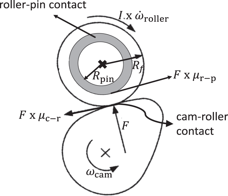

The preference of roller followers instead of sliding followers is nowadays more often made by manufacturers due to reduced friction losses and wear. ¹ In fact, the use of roller followers leads to a very small sliding velocity at the cam–roller contact. The latter is often referred as roller slip in the literature. Of course, the tribological designer's requirement of the cam–roller follower unit is such that the almost “pure-rolling” condition at the cam–roller contact should be maintained under all expected operating conditions.

Roller slippage has been the subject of a number of theoretical and experimental studies, see for instance Duffy, ² Khurram et al., ³ Chiu, ⁴ Ji and Taylor, ⁵ and Turturro et al. ⁶ As explained by Chiu ⁴ and also demonstrated in the experiments performed by Bair and Winer, ⁷ the magnitude of roller slip is strongly governed by the acting contact force, i.e. the higher the contact force the lower the magnitude of experienced roller slippage due to enhanced traction to drive the roller.

Chiu ⁴ and more recently Umar et al. ⁸ also showed that roughness effects play an important role in mixed friction calculations of the cam–roller contact. It is worth mentioning that the previously mentioned studies treated the asperity component of the mixed lubrication model using a statistical approach. Also, only lightly loaded cam–roller units (pressures up to 0.7 GPa approximately) were investigated. Tribological behavior of injection cam–roller follower units has been investigated by Lindholm et al. ⁹ ; however, their approach relies on semianalytical formulations for the mixed lubrication model.

Recently, Alakhramsing et al. ¹⁰ presented a full transient elastohydrodynamic (EHL) model for the coupled cam–roller and roller–pin contact. The aforementioned authors simulated a cam–roller follower unit as part of the fuel injection equipment of heavy-duty diesel engines and showed that a quasi-static analysis is justified for the considered application as transient effects are negligible. Also, the results showed that for low levels of friction in the roller–pin contact the sliding velocity at the cam–roller contact remains very small. Furthermore, the obtained film thickness profiles for the cam–roller contact suggested that the cam–roller contact operates in the mixed lubrication regime.

As mentioned earlier the sliding velocity, and thus also the slide-to-roll ratio (SRR), are strongly governed by the contact force. For the considered application of fuel injection cam–roller follower units, the SRR reaches values up to 10⁻⁶–10⁻⁵ in the nose region where the contact forces are the highest, ¹⁰ i.e. in the order of 15–17 kN. In rolling contact problems the SRR is often referred as the creep ratio, which is a more widely used term in vehicle dynamics. ¹¹

Due to the existence of a finite value of the SRR rather than a zero value, the contact area is divided into micro-stick and slip zones in dry rolling contacts, which are exposed to combined normal and tangential loading. A stick zone can be defined as two contacting elements or group of elements, which have no relative velocity with respect to each other, as they travel through the contact. In slip regions the aforementioned condition does not hold. In fact, when a tangential force is transmitted to the contact the contacting elements deform (elastically). The tangential force, which is related to the SRR, also causes a type of “rigid body displacement/ translation” throughout the contact. A slip element exists when the elastic deformation cannot support the displacement, i.e. the maximum tangential deformation is restricted with an upper limit of shear traction that has been reached. A sticking element is thus defined as to be when the acting shear stress over that element is less than the limiting shear stress. The most convenient way of defining the upper limit of shear traction is according to the Coulomb friction theory, i.e. the maximum (localized) shear traction is the product of normal pressure and a Coulomb friction coefficient. The moment the shear stress of an asperity exceeds this upper limit, the shear stress magnitude over the asperity is set equal to the upper limit. Gross sliding occurs at the moment when a sufficiently large SRR (and thus large tangential force) makes the entire contact area slip, i.e. when the stick area disappears.

In literature one may find several (tangential) contact models which are able to compute the shear stress distribution in dry rolling contacts. Carter et al. ¹² first described the continuum rolling theory. Later on Kalker ¹³ developed the linear theory. Afterward Johnson ¹⁴ and Vermeulen and Johnson ¹⁵ generalized Carter's theory to three dimensions. Kalker ¹⁶ also developed a “simplified theory,” which is implemented in FASTSIM, ¹⁷ a program which is widely used in wheel–rail contact problems. Also, Kalker's exact theory CONTACT ¹⁸ is widely used as a physical model, especially in wheel–rail contact problems. It is worth mentioning that all aforementioned tractive rolling contact models are based on smooth surfaces. Extension to study the “rough” tangential contact problem, based on real measured surface roughness, was made by Zhu and Olofsson ¹¹ and more recently by Xi et al. ¹⁹

Coming back to cam–roller follower contact modeling, the possibility exists that the stick–slip status of the cam–roller contact under such small SRRs has not yet reached the status of gross sliding, i.e. some contacting asperities may still be in the stick mode. Predicting the mixed frictional force for the cam–roller contact using a dynamic/sliding friction coefficient, also called boundary/asperity friction coefficient in literature, might therefore largely overestimate the friction force.

The problem of large discrepancies in predicted and measured traction coefficients for very low SRRs under mixed lubrication conditions, see for instance measurements in the work of Masjedi and Khonsari, ²⁰ was recently noticed and investigated by Xi et al. ²¹ In Xi et al. ²¹ the authors utilized the concept of a linear complementarity problem formulation ¹⁹ in order to solve the normal and tangential dry contact problem involving rough surfaces. Their conclusion was that assuming the contribution of the asperity friction contact component as a constant value, i.e. the corresponding sliding friction coefficient, might lead to an overestimation of the overall mixed friction coefficient in the low SRR domain.

From past literature one may notice that mixed lubrication (using measured surface roughness) in the low SRR domain, where stick–slip transitions are of importance in mixed friction predictions, is not extensively described. Therefore, this paper attempts to fill in this gap by presenting an efficient load-sharing-based mixed lubrication model, taking into account the real measured surface roughness and the stick–slip status of contacting asperities. As such, a special emphasis is laid on mixed friction predictions in the low SRR domain.

The model is applied to analyze the tribological behavior of a heavily loaded cam–roller follower contact. In this study we assume a friction coefficient for the roller–pin contact in order to assess the “sensitivity” of the cam–roller lubrication performance as a function of the lubrication performance of the roller–pin contact. According to the present author's knowledge such an analysis, especially applied to the coupled cam–roller and roller–pin contact, has not been carried out earlier. It can be imagined that an overestimation in friction force at the cam–roller contact will automatically lead to an (numerical) increase in the friction force in the roller–pin contact (due to the governing torque balance), leading to a different picture of the overall tribological behavior of the cam–roller follower unit.

Mathematical model: Mixed lubrication

This section describes the mathematical model including the theory and governing equations. In order to reduce the required computational effort, the exact axial shape of the interacting solids is not taken into account here. Instead, the pressure distribution in the axial direction is assumed to be uniform. This simplifies the problem to that of a classical “infinite” line contact problem, i.e. a 2D problem.

As mentioned earlier, in this paper we study the lubrication conditions of a cam–roller follower unit as part of the fuel injection equipment in heavy-duty diesel engines. In Alakhramsing et al. ¹⁰ the authors motivated that for this application a quasi-static analysis yields sufficiently accurate results. Hence, the model developed in this work also relies on quasi-steady conditions.

Mixed lubrication is treated according to the load-sharing formulation of Johnson et al., ²² i.e. in the mixed lubrication regime the total load is partly carried by the contacting asperities and partly by the fluid film. In equation form this is written as follows

$$F={\int }_{\Omega }(p_{\text{a}}+p_{\text{h}})\text{d}\Omega$$

(1)

where p_a and p_h denote the asperity and hydrodynamic pressure, respectively. Ω represents the computational domain.

In this work the considered sliding velocities at the cam–roller contact are very small, i.e. SRRs of less than 3% are considered. Hence, the model developed herein is developed assuming isothermal conditions. The complete mixed lubrication model follows a two-scale approach consisting of a smooth EHL model (macroscale) and a dry rough contact model (microscale), which are used to evaluate p_h and p_a, respectively. These two models are interrelated through the separating distance, which in turn depends on the film thickness.

The frictional coefficient acting on the contact includes contribution of lubricant and asperity shear stress

$$\mu =\frac{{\int }_{\Omega }(q+\tau )\text{d}\Omega }{F}$$

(2)

where μ is the friction coefficient, q is the asperity contact shear stress, and τ is the shear stress of the lubricant. The dry rough contact model solves for the asperity shear traction q, which determines the stick–slip status of the contacting asperities. As explained earlier, the stick–slip status of the contacting asperities ultimately influences the contribution of the asperity frictional force to the total mixed frictional force acting at the cam–roller contact. The mixed frictional force, acting at the cam–roller contact, largely determines the roller surface velocity (and thus the lubricant mean entrainment velocity of the cam–roller contact).

The two aforementioned submodels are described individually in the subsequent subsections.

Smooth EHL component

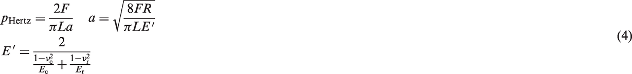
The isothermal line contact EHL model presented in this work is based on the finite element method (FEM) and stems from the pioneering work of Habchi et al. ²³ Typical EHL governing equations, applying to the cam–roller contact, are the Reynolds equation, the load balance equation, and the classical linear elasticity equations. For details pertaining the numerical procedure and finite element formulations and/or coupling of the governing EHL equations, the reader is asked to read Habchi et al. ²³ as only the main features are recalled here.

All EHL equations are presented in nondimensional form. Hence, the following dimensionless variables are introduced

$$\begin{array}{c}X=\frac{x}{a}Z=\frac{z}{a}{P}_{\text{h}}=\frac{p_{\text{h}}}{p_{\text{Hertz}}}\stackrel{\sim }{\eta }=\frac{\eta }{{\eta }_0}\\ \stackrel{\sim }{\rho }=\frac{\rho }{{\rho }_0}H=\frac{\mathit{hR}}{a^2}{H}_0=\frac{h_{0}R}{a^2}\hfill \end{array}$$

(3)

with Hertzian parameters defined as follows

$$\begin{array}{c}{p}_{\text{Hertz}}=\frac{2F}{\pi \mathit{La}}a=\sqrt{\frac{8\mathit{FR}}{\pi \mathit{LE}\text{'}}}\\ E\text{'}=\frac{2}{\frac{1-{\nu }_{\text{c}}^2}{E_{\text{c}}}+\frac{1-{\nu }_{\text{r}}^2}{E_{\text{r}}}}\hfill \end{array}$$

(4)

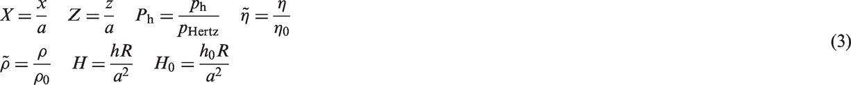
ρ and η denote the density and viscosity of the lubricant, respectively. L, $E\text{'}$ , and F are the axial length, reduced elasticity modulus, and contact force, respectively. Subscripts “c” and “r” denote cam and roller, respectively. $R=\frac{1}{\frac{1}{R_{\text{c}}}+\frac{1}{R_{\text{f}}}}$ represents the reduced radius of curvature. R_f and R_c are the outer radius of the roller follower and the cam radius of curvature (see Figure 1).

Figure 2 shows the equivalent EHL computational domain Ω for the cam–roller contact. In order to reduce computational effort an equivalent elastic domain Ω (with equivalent mechanical properties) is chosen in order to accommodate for the total elastic deformation $\stackrel{\sim }{\delta }$ . This avoids double calculation of the individual elastic deformations of the interacting solids. The dimensions of Ω, 60 × 60, are chosen such in order to mimic a half-space. ²³ To be more specific, in order to ensure that a zero elastic displacement field is attained in regions far away from the contact region Ω_f. Ω_f denotes the fluid film boundary on which the Reynolds equation is employed and has the dimensions of –4.5 ≤ X ≤ 1.5. Finally, Ω_d denotes the bottom boundary.

Figure 2.

Equivalent geometry for EHL analysis of the infinite line contact problem. The dimensions are exaggerated for the sake of clarity.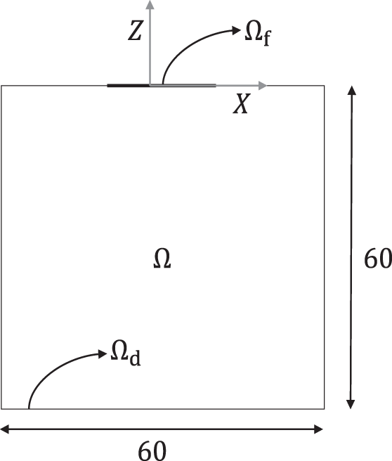

The hydrodynamic pressure distribution P_h in the contact is governed by the Reynolds equation, which is written as follows

$$\begin{array}{c}\frac{\partial }{\partial X}(-\frac{\stackrel{\sim }{\rho }{H}^3}{\stackrel{\sim }{\eta }\lambda }\frac{\partial P_{\text{h}}}{\partial X}+C_{u}H\stackrel{\sim }{\rho })=0\end{array}$$

(5)

where $\lambda =\frac{12U_{\text{c}}{\eta }_0{R}_{\text{x}}^2}{a^3{p}_{\text{Hertz}}}$ is a dimensionless speed parameter and $C_U=\frac{U_{\text{c}}+U_{\text{r}}}{2U_{\text{c}}}$ . Equation (5) includes the following features/assumptions:

• Variation of density and viscosity of lubricant with pressure is simulated using the well-known Dowson and Higginson ²⁴ and Roelands ²⁵ relations, respectively.

• The free boundary problem arising at the outlet of the contact is treated according to the penalty formulation of Wu. ²⁶

• Suitable residual-based numerical stabilization techniques, as detailed in Habchi et al., ²³ are employed in order to stabilize the solution at high loads.

• At the inlet of the contact fully flooded conditions are assumed.

The film thickness in the cam–roller contact is written as follows

$$\begin{array}{c}H(X)=H_0+\frac{X^2}{2}-\stackrel{\sim }{\delta }(X)\end{array}$$

(6)

where H₀ is the rigid body displacement and $\stackrel{\sim }{\delta }$ is the total elastic deformation of the interacting solids. As mentioned earlier, the calculation of $\stackrel{\sim }{\delta }$ is based on a 2D elasticity matrix. ²⁷

The rigid body displacement H₀ is obtained by satisfying the load balance, as defined by Johnson et al. ²²

$$\begin{array}{c}{\int }_{{\Omega }_f}P(X)\text{d}X={\int }_{{\Omega }_f}{P}_{\text{h}}(X)\text{d}X+{\int }_{{\Omega }_f}{\overline{P}}_{\text{a}}(X)\text{d}X=\frac{\pi }{2}\end{array}$$

(7)

where ${\overline{P}}_{\text{a}}$ represents the dimensionless dry “auxiliary” mean contact pressure, the calculation of which will be treated in the “Asperity contact component” section. The term “auxiliary” has deliberately been used here as ${\overline{P}}_{\text{a}}$ does not represent the actual asperity pressure distribution within the contact. Nevertheless, ${\overline{P}}_{\text{a}}$ links the microscale dry contact model to the macroscopic smooth EHL model. As mentioned before, this will be treated in the “Asperity contact component” section. P is the summation of the individual pressure distributions ${\overline{P}}_{\text{a}}$ and P_h and is called the total pressure distribution for the sake of clarity.

The smooth EHL model for the cam–roller contact is subjected to the following boundary conditions:

The pressure at the edges of the fluid flow boundary Ω _f equals zero.

A zero displacement condition is imposed at bottom of the boundary Ω_D.

For the elastic part a pressure boundary condition, with total pressure P, is imposed on the fluid flow boundary Ω _f .

On all remaining boundaries zero stress conditions are imposed.

Asperity contact component

The contact problem between two rough surfaces is translated into that of a rough surface (with equivalent mechanical properties) against a rigid flat surface. Suppose that the rigid flat surface indents the rough surface by a normal load F _z along the z-axis and tangential loads F _x and F _y are applied parallel to the x–y plane, then the contact interaction results in normal pressure p _a and shear tractions q _x and q _y in the interface. The general contact model, ²⁸ for steady-state rolling contacts, is repeated here for the sake of clarity

$$\begin{array}{c}{u}_z(x,y)=z(x,y)-h_{\text{s}}(x,y)\end{array}$$

(8a)

$$\begin{array}{c}\frac{{\stackrel{·}{s}}_x(x,y)}{0.5(U_{\text{c}}+U_{\text{r}})}={\xi }_x-\frac{\partial u_x(x,y)}{\partial x}\end{array}$$

(8b)

$$\begin{array}{c}\frac{{\stackrel{·}{s}}_y(x,y)}{0.5(U_{\text{c}}+U_{\text{r}})}={\xi }_y-\frac{\partial u_y(x,y)}{\partial y}\end{array}$$

(8c)

where u _x , u _y , and u _z are the deformation components along the x, y, and z axes, respectively. z(x, y) represents the roughness profile and h_s (x, y) the separating distance. ξ _x and ξ _y are the longitudinal and lateral creepages, respectively, i.e. s _x and s _y are the relative slip distances parallel to the x and y axes, respectively. In this study the tangential load F _y is assumed to be zero at all times. Hence, for the current study only unidirectional creep is considered and thus ξ _y  = 0. Note that the longitudinal creep ratio ξ _x is nothing else but the SRR, i.e. ${\xi }_x=\text{SRR}=\frac{U_{\text{c}}-U_{\text{r}}}{0.5(U_{\text{c}}+U_{\text{r}})}$ .

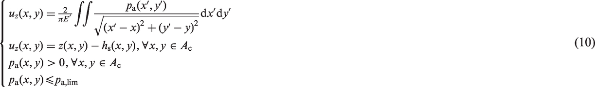
In order to solve the rough contact problem subjected to both normal and tangential loads under the stick–slip condition, one should first solve for the distribution of the asperity normal contact pressure p_a. For the current analysis it is assumed that all interacting solids share similar material properties. Hence, we can safely neglect the influence of tangential tractions q _x and q _y on relative normal displacement, and thus normal contact geometry and pressure distribution p_a. ²⁹ With this simplification the normal contact pressure distribution p_a becomes an input for tangential contact problem (also known as the stick–slip problem).

The complete dry contact model, including both normal contact pressure p_a and shear traction analysis q _x and q _y , is a boundary element method (BEM)-based model. In fact, for the normal contact pressures p_a calculation the elastic–perfectly plastic contact model of Akchurin et al. ³⁰ is employed. For the tangential contact problem, the model of Bazrafshan et al. ³¹ is employed. Note that the model described in Bazrafshan et al. ³¹ assumes purely elastic contacts. In the current analysis it is assumed that the occurring shear stresses are insignificant to cause yielding. Hence, for the normal contact pressure p_a analysis an elastic–ideal plastic material model is used, while for the shear stress q analysis a purely elastic model is used.

The complete contact model is used to calculate the local dry/solid contact pressures and shear stresses of a representative section of the real measured surface topography. In fact, the contact model is based on the Boussinesq-Cerruti integral equations, ²⁸ which relate surface tractions to displacements. For the sake of simplicity the localized hardness and Coulomb friction law are defined as to be the upper limits of contact pressure and shear traction, respectively.

The iterative conjugate gradient method, with the assistance of the discrete convolution and fast Fourier transform algorithm, is employed to efficiently determine the unknown contact and stick area. The complete solution of the dry contact model includes the real contact area, pressure p_a, stick areas, and tangential tractions q _x and q _y .

Now that the general features of the dry contact model are described, its relation to the macroscopic mixed lubrication model can be treated. Hence, this subsection is divided into two parts. The first part treats the relation of the asperity contact pressure distribution p_a to the macro-setting of the mixed lubrication model. The second part is devoted to the stick–slip problem, i.e. calculation of the local shear tractions q _x , q _y and its relation to the macro-setting of the mixed lubrication model.

Normal contact

The earlier described dry contact model is used to calculate the asperity contact pressures of a representative section of the real measured surface topography. The computational grid size for the contact model contained N _x  × N _y  = 250 × 250 data points at intervals of 0.5 µm. The dimensions of the dry contact model calculation domain, which is used to solve for p_a, are L _x  × L _y (for x- and y-direction, respectively). Note that this is the microscale dry contact model calculation domain and should not be confused with the macroscale fluid film domain Ω_f. Periodic boundary conditions are imposed at the edges of the dry contact model calculation domain to calculate the representative section. For both roller and cam, a randomly chosen area was used to measure the surface roughness. To give an indication, the R _a values for the measured surface roughness of cam and roller positions are 0.135 and 0.095 µm, respectively.

Furthermore, the dry contact model relies on a linear elastic–perfectly plastic material model. Hence, the allowable contact pressures are therefore limited to a pressure p_a,lim at which plastic flow occurs. p_a,lim is therefore an input parameter to the contact model.

The methodology used here to obtain the proportion of load carried by the asperities has been introduced by Bobach et al. ³² This approach will briefly be explained now.

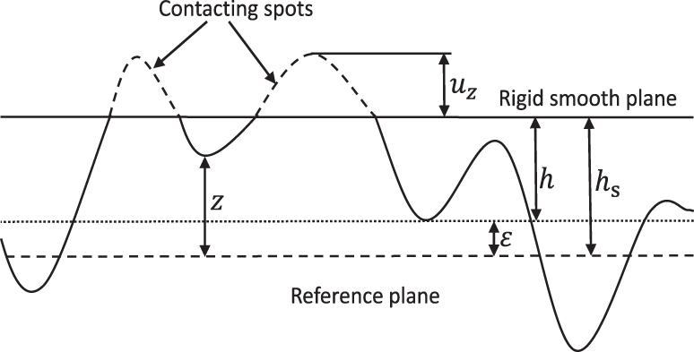
In the mixed lubrication model a separation distance h_s is required to calculate the asperity contact pressure distribution p_a (see Figure 3). The contacting asperities fully penetrate the EHL bulk lubricant film. As defined by Johnson et al., ²² the condition of volume conservation relates the separating distance h_s is related to the film thickness h. To be more specific, h_s should fulfill the condition that the total lubricant volume between the smooth surfaces should be equal to the volume occupied by the pockets formed by the noncontacting parts between the rough surfaces. In fact, the separation distance h_s has the same shape as the film thickness h but with a constant offset ε so that volume conservation is preserved (see Akchurin et al. ³⁰ for more details), as can be inferred from Figure 3. The offset ε is obtained iteratively in the asperity contact model, by satisfying the following equation

$${\int }_{A}h(x,y)\text{d}A=\int {\int }_{\stackrel{\sim }{A}}(h_{\text{s}}(x,y)-z(x,y)+u_z(x,y))\text{d}\stackrel{\sim }{A}$$

(9)

where A is the total area and $\stackrel{\sim }{A}$ is the lubricated area. The set of equations, to be solved for the dry contact model, are

$$\begin{array}{c}\{\begin{array}{c}{u}_z(x,y)=\frac{2}{\pi E^{\text{'}}}\int \int \frac{p_{\text{a}}(x\text{'},y\text{'})}{\sqrt{(x\text{'}-x{)}^2+(y\text{'}-y{)}^2}}\text{d}x\text{'}\text{d}y\text{'}\\ u_z(x,y)=z(x,y)-h_{\text{s}}(x,y),\forall x,y\in A_{\text{c}}\\ p_{\text{a}}(x,y)>0,\forall x,y\in A_{\text{c}}\\ p_{\text{a}}(x,y)\le p_{\text{a},\text{lim}}\end{array}\end{array}$$

(10)

Figure 3.

Schematic view of the surfaces which are in contact. z(x, y) represents the surface roughness profile, h_s the separating distance, and the deflection u _z .

For the dry contact model the unknowns are p_a (x, y) and A_c, whereas h_s is related to the film thickness according to equation (9). Now, one may define an auxiliary mean asperity contact pressure ${\overline{p}}_{\text{a}}$ (over calculation domain L_xL_y) as follows

$${\overline{p}}_{\text{a}}=\frac{1}{L_x{L}_y}\int \int p_{\text{a}}(x,y)\text{d}x\text{d}y=\frac{F_z}{L_x{L}_y}$$

(11)

Now we may establish a functional curve of ${\overline{p}}_{\text{a}}$ versus h _s (and indirectly h) (see Figure 4). In fact, we basically define a precalculated relation between auxiliary mean asperity contact pressure ${\overline{p}}_{\text{a}}$ and film thickness h, by assuming nominally flat surfaces in contact, so that

$$\begin{array}{c}{\overline{p}}_{\text{a}}(x)=f[h(x)]\end{array}$$

(12)

Figure 4.

Relationship between the auxiliary mean asperity contact pressure ${\overline{p}}_{\text{a}}$ and film thickness h.

Equation (12) can be interpreted as a relation describing the “stiffness” of the contact, which describes the influence of the measured surface roughness. For the sake of simplicity, we call curve depicted in Figure 4 as the “ $h-{\overline{p}}_{\text{a}}$ curve” throughout this paper. It should be noted that equation (12) can be used to evaluate any dry auxiliary mean contact pressure for any film thickness in the macroscopic setting of the mixed lubrication model.

The precalculated relationships equation (12) always holds for the specific measured contact pair (which is chosen as representative section of the interacting components). The assumption here is that the surface topography does not change in time (which, for example, is the case in running-in of components). Also note that in this study we only deal with highly loaded contacts, meaning an almost uniform film thickness distribution within the contact zone, which also justifies the usage of nominally flat surfaces in contact for the precalculation of the relationship given by equation (12).

So, the developed model in this work basically “lumps/averages” the micro-effects and uses this information in the macroscopic setting of the lubrication model, for mixed friction calculations. The current method offers a more deterministic approach as it uses information from real measured surface roughness.

For usage in the load balance equation (7), the dimensionless dry auxiliary mean asperity contact pressure ${\overline{P}}_{\text{a}}$ is computed as follows

$$\begin{array}{c}{\overline{P}}_{\text{a}}(x)=\frac{{\overline{p}}_{\text{a}}(x)}{p_{\text{Hertz}}}\end{array}$$

(13)

Tangential contact

For the cam–roller contact, the film thickness/separation may be nonuniform and also varies as a function of the cam angle. Also, the SRR varies as a function of cam angle. In order to solve the tangential contact problem, the surface roughness, normal load F _z , and SRR are required. However, the way the set of equations (8b) and (8c) are formulated, the complete tangential cam–roller contact problem needs to be solved each time. This would require huge computational effort, especially when simulating the whole cam's lateral surface. It is therefore wishful to employ a similar strategy as employed for the normal contact problem. Meaning, to establish a precalculated relationship between the tangential force F _x , film thickness h, and SRR, for nominally flat surfaces in contact. This relationship should always hold for the specific contact pair corresponding to the prespecified surface roughness profiles. The strategy followed will be explained now.

Tangential contact: Two nominally flat surfaces in contact

As the idea here is to relate the tangential force F _x to the film thickness h in the context of stick–slip transitions we consider, similar as was done for the normal contact problem, two nominally flat surfaces in contact. As the asperity contact pressure distribution p_a is already calculated for the normal contact problem for a given h, transmission of force F _x will induce an additional rigid body translation δ _x in x-direction, which needs to share a similar magnitude as the asperity tangential deformation u _x , for asperities in stick mode. This is evident from the general contact model (for two interacting components at rest, transmitting tangential force F _x )

$$\begin{array}{c}\begin{array}{c}{s}_x(x,y)=u_x(x,y)-{\delta }_x\\ s_y(x,y)=u_y(x,y)-{\delta }_y\end{array}\end{array}$$

(14)

The stick–slip code adapted here from Bazrafshan et al. ³¹ can be employed to solve the set of equations (14) for rough surfaces. From the normal asperity contact pressure analysis described earlier, the real contact area A_c is obviously also automatically evaluated. Note that the normal pressure acting on the asperity in this model is solely p_a. One should not confuse ${\overline{p}}_{\text{a}}$ with p_a as ${\overline{p}}_{\text{a}}$ is an auxiliary pressure and not the actual asperity contact pressure. The aforementioned should be stressed, especially due to its importance when formulating the asperity shear stress q.

The contacting elements are defined to be those where the asperity contact pressure is greater than zero, i.e. $p_{\text{a}}(x,y)>0,\forall x,y\in A_{\text{c}}$ . The real contact area A_c is composed of stick zones A_st and slip zones A_sl, which are defined as follows

$$\begin{array}{c}\begin{array}{c}\{|q{|}_{(x,y)}\le {\mu }_{\text{a}}{p}_{\text{a}(x,y)},|s{|}_{(x,y)}=0\},\forall x,y\in A_{\text{st}}\\ \{|q{|}_{(x,y)}={\mu }_{\text{a}}{p}_{\text{a}(x,y)},|s{|}_{(x,y)}\ne 0\},\forall x,y\in A_{\text{sl}}\end{array}\end{array}$$

(15)

where $|q{|}_{(x,y)}=\sqrt{|q_x{|}_{(x,y)}^2+|q_y{|}_{(x,y)}^2}$ and $|s{|}_{(x,y)}=\sqrt{|s_x{|}_{(x,y)}^2+|s_y{|}_{(x,y)}^2}$ are the shear stress and relative slip magnitudes, respectively. There is no direct metal-metal contact between contacting asperities due to the presence of boundary layers. μ_a is the Coulomb friction coefficient, which governs the friction a of the boundary layers. Basically equation (15) states that in the stick region the shear stress magnitude is less than the static friction and the relative slip distance is zero. The upper limit of shear traction is formulated according to the Coulomb friction theory, i.e. $|q_{\text{max}}{|}_{(x,y)}={\mu }_{\text{a}}{p}_{\text{a}(x,y)}$ . The moment the shear stress of an asperity exceeds this upper limit, the shear stress magnitude over the asperity is set equal to the upper limit and micro-slip occurs. This is the most simple way of defining the upper limit for shear traction of the stick–slip problem, for opposing materials with similar mechanical properties. For stick–slip problems involving interacting solids with different hardness values, the upper limit shear stress is often assumed to be governed by hardness of the softer material. ³³

The model inputs for the stick–slip model include μ_a, material mechanical properties, and normal loads F _z . The tangential load F _x is defined as follows

$$F_x={\mu }_{\text{a}}{F}_z$$

(16)

Note that u _y is zero as F _y is zero.

A suitable initial guess for the rigid tangential translation δ _x is assumed and fed to the model. δ _x is iteratively adjusted so that the numerical integration of q _x (x, y) over the calculation domain is equal to the specified tangential force F _x , as given by equation (16).

If μ_a is increased gradually at a constant normal load F _z , then a transition curve from static to sliding friction, as a function of δ _x , can be obtained. The sliding friction coefficient, alternatively known as the asperity friction coefficient μ_a,lim, can be determined experimentally from a pin on disc setup, for example. The asperity friction coefficient μ_a,lim should serve as an upper limit for the transition curve. Hence, for the present study μ_{a, lim} is a model input parameter. In Figure 5 a schematic of such a transition curve is illustrated. Note that when μ_a = μ_a,lim gross sliding takes place and A_st = 0. It is worth mentioning that in this study quasi-static conditions are assumed, i.e. the loading process is slow and thus inertia effects are neglected here.

Figure 5.

Relationship between μ_a and δ _x , mapped against normal load F _z . Notice all curves merging at limiting friction coefficient μ_a,lim.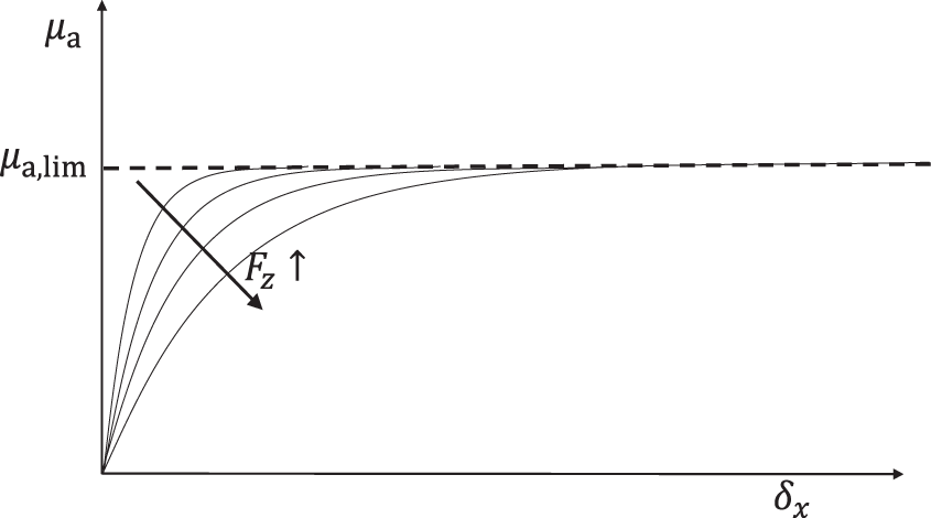

Figure 5 also depicts what happens when the normal load F _z is varied. It is obvious that when F _z is increased, i.e. the surfaces are pressed harder against each other, the distance before gross sliding takes place increases as more asperities remain in the stick mode.

Analogously to equation (12) it is possible to define an auxiliary asperity shear stress $|\overline{q}|$ as follows

$$\begin{array}{c}|\overline{q}|=\frac{1}{L_x{L}_y}\int \int |q{|}_{(x,y)}\text{d}x\text{d}y=\frac{F_x}{L_x{L}_y}\end{array}$$

(17)

Note that likewise ${\overline{p}}_{\text{a}},|\overline{q}|$ does not represent the actual asperity shear traction distribution within the contact. Nevertheless, the purpose of using $|\overline{q}|$ is to link the microscale dry contact model to the macroscopic smooth EHL model as will be shown now. First, equation (16) is rewritten as follows

$$\begin{array}{c}{\mu }_{\text{a}}=\frac{|\overline{q}|}{{\overline{p}}_{\text{a}}}\end{array}$$

(18)

Equation (18) creates the possibility to relate the friction coefficient μ_a to the film thickness h according to equation (12). Finally, it now becomes possible to establish a precalculated relationship between μ_a, the film thickness h, and the rigid tangential translation δ _x , from the stick–slip code, as follows

$$\begin{array}{c}{\mu }_{\text{a}}=f[h,{\delta }_x]\end{array}$$

(19)

It should be noted that equation (19) can be used to evaluate any (asperity) friction coefficient for any film thickness (separation) and rigid tangential translation (for the specific contacting surface roughness profiles). In fact, for each film thickness h (corresponding to a normal load F _z ) a rigid tangential translation δ _x may be obtained by gradually increasing μ_a. The aforementioned procedure is then repeated for different film thicknesses. Hence, a precalculated 3D map, relating μ_a, h, and δ _x can be constructed and be used as an input for mixed friction calculations.

Tangential contact: Relation of two nominally flat surfaces tangential contact problem to the macroscopic rolling contact problem

Note that equation (19) describes the relationship between μ_a, h, and δ _x . However, for the macroscopic rolling contact problem the SRR is another variable which needs to be considered. The relationship between SRR and the “rigid tangential displacement” δ _x will be explained now. In order to observe the direct relationship between shear stress and tangential displacements, the rolling contact equations (8b) and (8c) are integrated with respect to x

$$\begin{array}{c}\begin{array}{c}{s}_x(x,y)={\xi }_{x}x-u_x(x,y)-C_1(y)\\ s_y(x,y)={\xi }_{y}x-u_y(x,y)-C_2(y)\end{array}\end{array}$$

(20)

where again ξ _x  = SRR and C₁ and C₂ are values generated from the integration. Note that for the current case ξ _y  = 0 as F _y  = 0 N. According to Kalker's simplified theory, ¹⁶ C₁ and C₂ are zero as the surface tractions q _x and q _y are zero at the leading edge of the contact. If now one compares equations (14) and (20) then the macroscopic rigid body displacement for the rolling contact takes the form of ξ_xx, i.e. SRR ⋅ x. To be more specific, the rigid body tangential displacement δ _x as a function of x, in the macroscopic mixed lubrication model, is approximated as follows

$${\delta }_x(x)=\text{SRR}·x$$

(21)

So, for each value of x in the contact zone of the macroscopic mixed lubrication model a corresponding value of μ_a can be deduced from the precalculated 3D map relating μ_a, h, and δ _x (according to equation (19)).

Assuming that the starting point of the ${\overline{p}}_{\text{a}}(x)$ curve is x = x_inlet, then δ _x (x) within the contact zone can be redefined as follows

$${\delta }_x(x)=\text{SRR}·(x-x_{\text{inlet}})$$

(22)

At this point it is worth noting that the starting point of the ${\overline{p}}_{\text{a}}(x)$ curve usually is not x_inlet = –a, i.e. the extent of the effective contact region will usually be larger than 2a, as still some asperity contact may occur outside the dry Hertzian half-width contact region (in mixed lubrication). Greenwood et al. ³⁴ defined a parameter $\alpha =\frac{\sigma R}{a^2}$ , which serves as a measure of the influence of roughness on the Hertzian deformation. σ is the combined roughness of the two surfaces. In fact, for 0 < α < 0.05, Greenwood et al. ³⁴ claim that the error between the rough and smooth solution is less than 7%. For all calculations in this analysis the aforementioned condition holds. Hence, for the current analysis x_inlet = –a can safely be used.

Once SRR and h(x) are known in the macroscopic mixed lubrication model, then μ_a (x) can be obtained by means of the precalculated 3D asperity friction map, relating μ_a, h, and δ _x . In fact, for the macroscopic rolling contact problem equation (19) may be reformulated as follows

$${\mu }_{\text{a}}(x)=f[h(x),{\delta }_x(x)]$$

(23)

where δ _x (x) is given by equation (22).

Calculation of roller surface velocity

The hydrodynamic shear stress τ is computed as follows

$$\begin{array}{c}\tau =-\frac{a{p}_{\text{Hertz}}}{R}\frac{H}{2}\frac{d{P}_{\text{H}}}{\text{d}X}+\frac{{\eta }_{0}R}{a^2}\frac{\stackrel{\sim }{\eta }(U_{\text{c}}-U_{\text{r}})}{H}\end{array}$$

(24)

Due to the very high pressures, which the cam–roller contact is subjected to, it is necessary to account for nonlinear viscous effects even at low SRRs. For the friction model developed here the Eyring model ³⁵ is adapted. Note that the Reynolds equation (5) does not take into account non-Newtonian behavior as the expected shear rates are such low that its effect on film thickness and pressure distribution is assumed to be negligible. Now that the asperity component friction coefficient (given by equation (19)) is defined, the mixed friction coefficient for the cam–roller contact μ_c–r can be obtained as follows

$$\begin{array}{c}{\mu }_{\text{c}-\text{r}}=\frac{\mathit{aL}}{F}{\int }_{{\Omega }_{\text{f}}}({\tau }_0{\mathit{sinh}}^{-1}(\frac{\tau }{{\tau }_0})+{\mu }_{\text{a}}{\overline{P}}_{\text{a}}{p}_{\text{Hertz}})\text{d}\Omega \end{array}$$

(25)

where subscript “c–r” corresponds to the cam–roller contact and L is the axial length of the contact. Note that the Erying friction law is directly incorporated in equation (25), i.e. τ₀ is the characteristic Eyring shear stress. It is also important to stress here that the asperity component friction coefficient μ_a is also a function of X, as defined by equation (19). At this point it is again worth stressing that ${\mu }_{\text{a}}{\overline{P}}_{\text{a}}{p}_{\text{Hertz}}$ represents an up-scaling of actual shear contribution of asperities q (as defined by equation (15)) to the macroscale.

The torque balance, which governs the roller surface velocity U_r is written as follows (see Figure 1)

$$\begin{array}{c}\underset{\text{tractivetorque}}{\underbrace{{\mu }_{\text{c}-\text{r}}{R}_{f}F}}=\underset{\text{resistingtorque}}{\underbrace{{\mu }_{\text{r}-\text{p}}{R}_{\text{pin}}F}}+\underset{\text{inertiatorque}}{\underbrace{I{\stackrel{·}{\omega }}_{\text{r}}}}\end{array}$$

(26)

where subscript “r–p” corresponds to the roller–pin contact, R_pin is the pin radius, and ω_r is the roller rotational velocity. In this study we consider only conditions where SRR < 3%. Hence, ω_r can be estimated assuming pure rolling conditions and ${\stackrel{·}{\omega }}_{\text{r}}$ can directly be obtained from graphical differentiation of ω_r (with respect to time).

In this study the influence of the lubrication conditions at the roller–pin contact is studied, in terms of its friction coefficient μ_r–p, on the lubrication performance at the cam–roller contact. Hence, μ_r–p is an input parameter.

Numerical procedure

Figure 6 depicts the solution flow chart for the mixed lubrication model which has been developed for the cam–roller contact. In the simplified asperity contact modeling approach adapted here (“Asperity contact component” section), the asperity contact pressure ${\overline{P}}_{\text{a}}$ is a direct function of the film thickness H. Furthermore, the asperity component friction coefficient μ_a is also a direct function of film thickness H and rigid tangential body translation δ _x (see equation (21)). The precalculated $h-{\overline{p}}_{\text{a}}$ curve ( ${\overline{p}}_{\text{a}}(x)=f[h(x)]$ ) and asperity contact friction transition map $({\mu }_{\text{a}}(x)=f[h(x),{\delta }_x(x)])$ are valid at all times for the specific contacting surface roughness profiles studied.

Figure 6.

Numerical solution scheme for the cam–roller lubrication model. BEM: boundary element method; FEM: finite element method.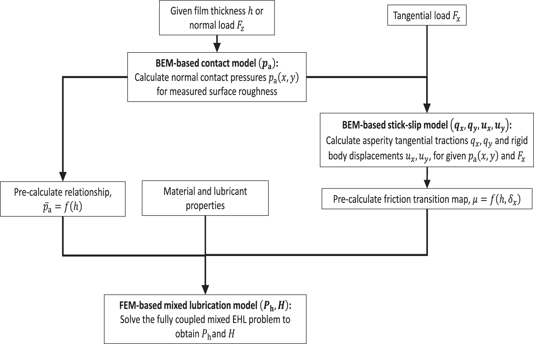

Therefore, the unknowns of the FEM-based mixed lubrication model are $(P_{\text{h}},\stackrel{\sim }{\delta },H_0,U_{\text{r}})$ . Note that $\stackrel{\sim }{\delta }=\{U,W\}$ is elastic displacement vector, where U and W are deformation components in X- and Z-direction, respectively.

The problem is formulated as a set of strongly coupled nonlinear partial differential equations. The resulting system of nonlinear equations is then solved using a monolithic approach where all the dependent variables (P_h, U, W, H₀, U_r) are collected in one vector of unknowns and simultaneously solved using a Newton–Raphson iterative scheme. Convergence is achieved according to user-specified tolerances. For specific numerical details pertaining to the weak finite element formulation of the governing equations and mesh element size distribution, see Habchi et al. ²³ and Alakhramsing et al. ³⁶ as only the main features are recalled here.

Results

The lubricant, material, and geometrical properties of the heavily loaded cam–roller follower unit, analyzed in this study, are listed in Table 1. The analyzed cam–roller follower unit is part of the fuel injection system in heavy-duty diesel engines. The listed material and geometrical properties are similar to those presented in Alakhramsing et al. ¹⁰

Table 1.

Reference operating conditions and geometrical parameters for cam–roller follower lubrication analysis.

Parameter	Value	Unit
E c	200	GPa
E r	200	GPa
ν c	0.3	–
ν r	0.3	–
ρ 0	870	kg/m3
α	1.84E-8	Pa−1
η 0	0.013	Pa s
τ 0	5	MPa s
R f	0.018	m
R pin	0.0091	m
L	0.021	m
μ a,lim	0.12	–
p a,lim	6	GPa

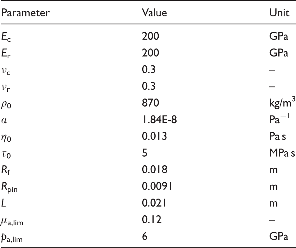
Figure 7(a) shows the calculated $h-{\overline{p}}_{\text{a}}$ curve which has been deduced by means of the mathematical model described in the “Asperity contact component” section. Again, the $h-{\overline{p}}_{\text{a}}$ curve provides the relationship between the film thickness h and auxiliary mean asperity contact pressure ${\overline{p}}_{\text{a}}$ , which always holds for measured surface roughnesses which were used as input for the dry contact model.

Figure 7.

(a) Calculated “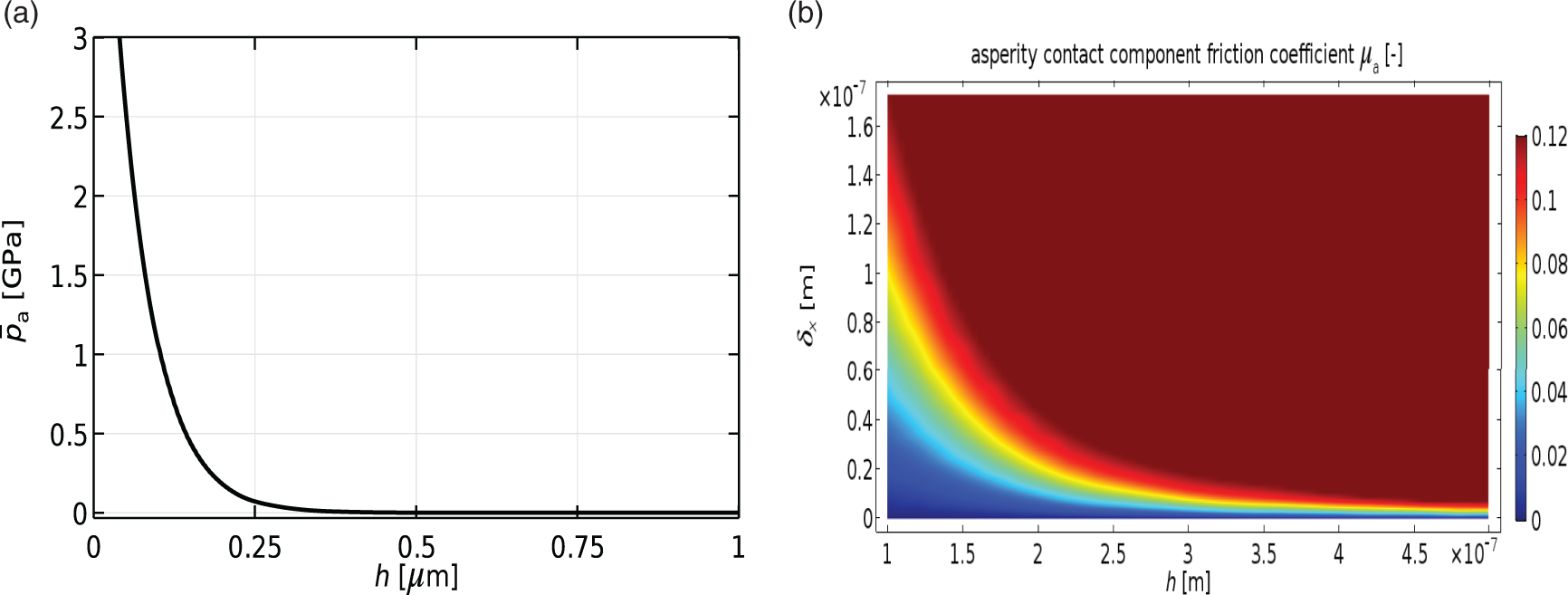 $h-{\overline{p}}_{\text{a}}$ curve” and (b) 3D map for the asperity contact friction coefficient μ_a as a function of the film thickness h and rigid tangential displacement δ _x .

Similarly, Figure 7(b) presents the calculated map for the asperity contact friction coefficient μ_a as a function of the film thickness h and rigid body tangential translation δ _x , which has been obtained from the stick–slip model. One can directly observe the major characteristics of this asperity friction transition map. To elaborate somewhat, for a decreasing film thickness (thus for increasing normal contact loads) the distance δ _x before gross sliding takes place increases. This is expected since with increasing normal loads the asperity contact area increases, so that a larger pre-(gross) sliding distance δ _x is required.

The precalculated Figure 7(a) and (b) serves as input to the (macroscopic) mixed lubrication model (as discussed earlier by means of Figure 6). In fact, the asperity friction map is specified in n data points for different combinations of h and δ _x . The n data points are spline interpolated with respect to h and δ _x , i.e. the discrete relation according to equation (19) is interpolated to obtain a third-order piecewise continuous polynomial fit for μ_a versus h and δ _x . A similar procedure was utilized, but then in 2D, in order to obtain the $h-{\overline{p}}_{\text{a}}$ curve.

Parametric sweep: The influence of roller–pin friction

In this section a parametric sweep is carried out in order to assess lubrication conditions at the cam–roller contact as a function of lubrication conditions in the roller–pin contact. This exercise is carried out here by means of a specified friction coefficient at the roller–pin contact. In the ideal situation the friction coefficient at the roller–pin contact, which could be classified as a lubricated journal bearing, would be dependent on the applied load. The roller–pin contact has been modeled in Alakhramsing et al. ¹⁰ in which extremely low levels of friction in the order of 0.003 were calculated. In unideal situations the frictional behavior at the roller–pin contact may increase due to external factors such as insufficient oil supply (starvation), manufacturing errors (deviation in tolerances), misalignment, particle entrapment, etc. Detailed investigation into the external factors is beyond the scope of the present study. From a designers perspective it is interesting to assess the “sensitivity” of cam–roller lubrication performance as a function of the lubrication performance in the roller–pin contact. This is done here by assuming a friction coefficient at the roller–pin contact. This assessment might provide useful insight into the coupled tribological behavior of the two contacts. Note that the friction coefficient at the roller–pin contact is independent of the applied load in this study, i.e. the resisting torque at roller–pin contact is independent from the load.

As this paper deals with the relation between roller slippage and the variable asperity coefficient μ_a (see equation (21)), it is interesting to assess two positions on the cam, namely: (i) the base circle, where the contact forces are the lowest and (ii) the nose where the contact forces are the highest. As explained earlier in the “Introduction” section, the contact force directly influences the sliding velocity via the torque balance equation (26). As discussed in earlier works,^10,36 a higher contact force induces a larger tractive torque and thus less roller slippage.

Hence, for the current analysis we consider lubrication conditions at the base circle and nose position. The operating conditions are listed in Table 2 and correspond to a cam rotational velocity ω_c of 950 r/min.

Table 2.

Reference operating conditions for base circle and nose position.

Position	F (N)	R (m)	uc (m/s)
Base circle	2250	0.0152	4.62
Nose	12,500	0.0105	3.98

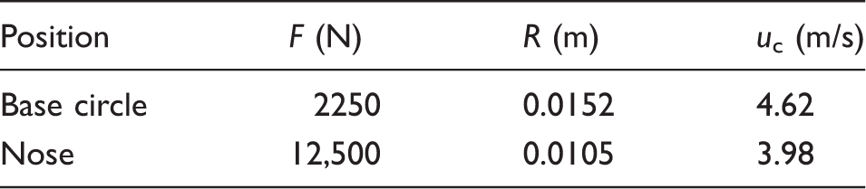
Figure 8(a) presents the hydrodynamic, asperity, and total pressure distributions, together with the dimensionless film thickness distribution for the nose position, with μ_r–p = 0.013. Note that these profiles do not capture the actual distribution of the asperity and lubricant pressure. However, they do provide important information regarding the fraction of load carried by asperities/lubricant and also regarding the film thickness/separation. The film thickness distribution provides information at which locations there may be potential asperity contact. From Figure 8(a) it is evident that for the considered operating conditions the asperity component pressure distribution is a small fraction of the total pressure distribution. Furthermore, when carefully looked, one may observe that still some asperity interaction occurs near the outlet of the contact as the asperity contact pressure distribution spans out further than the hydrodynamic pressure distribution. This effect is amplified in more mixed lubrication conditions (see for instance Masjedi and Khonsari ³⁷ ).

Figure 8.

(a) Pressure, film thickness, and (b) shear traction distributions for nose position, with μ_r–p = 0.013.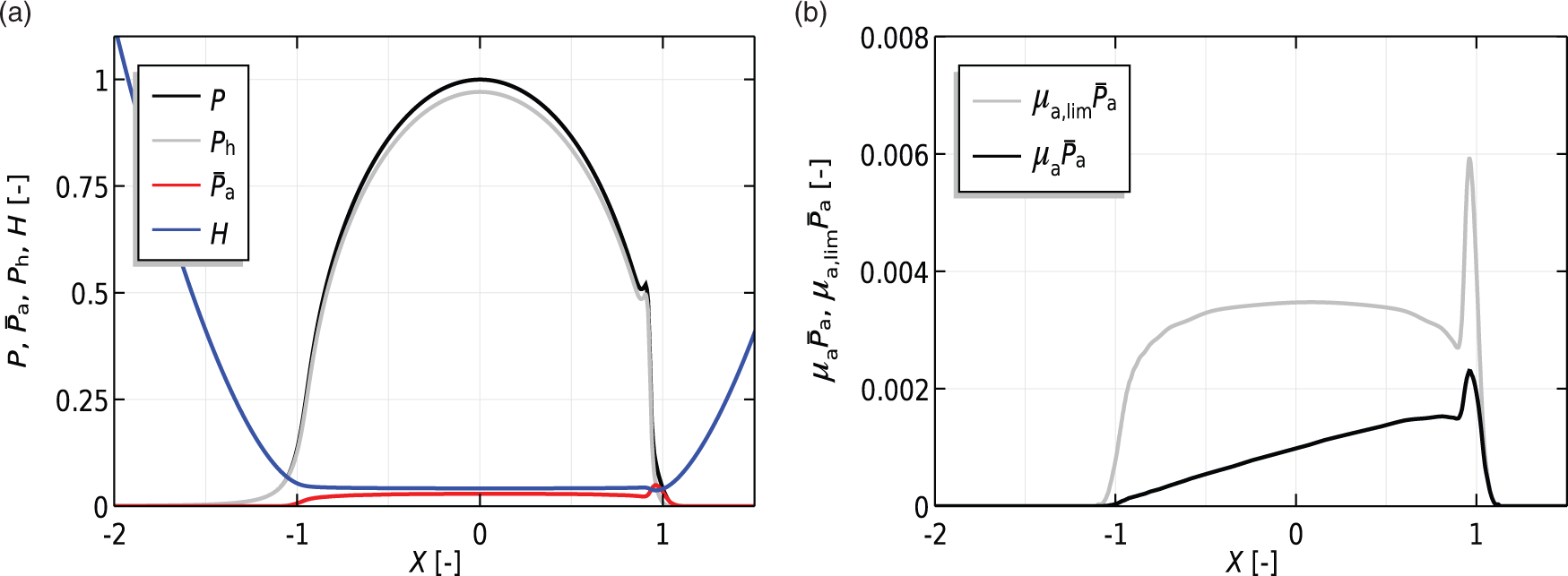

As can be seen from Figure 8(b) gross sliding has not yet been attained, for μ_r–p = 0.013, as the current asperity traction distribution ${\mu }_{\text{a}}{\overline{P}}_{\text{a}}$ has not fully filled up the traction bound ${\mu }_{\text{a},\text{lim}}{\overline{P}}_{\text{a}}$ yet. Furthermore, from Figure 8(b) classical features of smooth rolling contacts may be observed, i.e. in the static friction regime, the traction distribution starts from a zero value at the leading edge of the contact and increases throughout the contact until the gross sliding condition (μ_a (x) = μ_a,lim) has been met. It is worth mentioning that the traction does not increase linearly, which for instance is the case for Kalker's simplified theory. ¹⁶ The shear traction displacement relationship is a nonlinear one which is reflected in the 3D map relating μ_a, h, and δ _x (see Figure 7(b)).

Simulations are carried out in which the roller–pin friction coefficient μ_r–p is increased from 0.001 with increments of 0.001. The simulations are stopped whenever a SRR of 3% is reached.

Figure 9(a) provides the relation between increasing values of μ_r–p and SRR, for the nose position. In this figure the stick–slip results (meaning a variable asperity friction coefficient according to Figure 7(b)) are compared with those obtained by assuming the asperity friction coefficient to be a constant and equal to μ_a,lim, i.e. assuming gross sliding. Note that SRR and δ _x (x) are mutually dependent on equation (22) altogether with Figure 7(b). It is also worth explaining that an increase in μ_r–p means that μ_c–r automatically needs to increase proportionally. To do so, the sliding velocity needs to increase. Note that for the current application an increase in sliding velocity means a decrease in sum velocity. With this it is obvious that an increase in μ_r–p leads to an increase in δ _x (x) and thus also μ_a (x). Understanding this makes the interpretation of Figure 9(a) a lot easier.

Figure 9.

Influence of μ_r–p on lubrication conditions at (a) and (b) nose position and (c) and (d) base circle position. SRR: slide-to-roll ratio.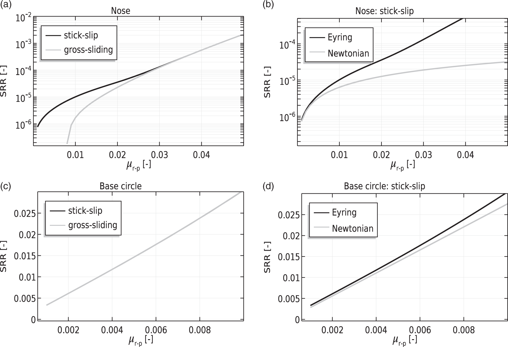

Initially for low values of μ_r–p, due to the extremely high contact force the sliding velocity is naturally very small, leading to a small rigid tangential displacements δ _x (x). Note that during the full parametric sweep the central film thickness, which is largely dependent on the sum velocity, remains constant at SRR < 3%. For the nose position the central film thickness is approximately 0.27 µm. So for the initial values of μ_r–p, the combination of h and δ _x (x) (see Figure 9(a)) reveals that the gross sliding inception has not occurred yet, i.e. some asperities are still in the stick mode. Hence, the μ_a (x) is still lower than μ_a,lim. As μ_r–p is increased further SRR increases, and so does δ _x (x), up to the inception of gross sliding, which automatically explains the unification of the curves depicted in Figure 9(a). Nevertheless, the difference between the obtained results, especially for low values of μ_r–p, is large. Assuming a constant asperity friction coefficient would lead to large overestimation in the friction coefficient for both cam–roller and roller–pin contact. At this point it is worth to remember that simulations were carried out with a starting value of μ_r–p = 0.001 and gradually increased. However, if one takes the look at Figure 9(a), then it is clear that under the assumption of gross sliding the value of μ_r–p = 0.001 is never attained for the gross sliding case. This can be explained as follows: the analysis here is carried out such that the shape of the film thickness/separating distance is hardly affected, i.e. the considered sliding velocities are very small. This implies that the load carried by the asperities is also hardly affected (see equation (12)). Now as earlier explained, for a given μ_r–p, the only thing which may be affected is the sliding velocity. If one assumes gross sliding, i.e. μ_a (x) = μ_a,lim, then the asperity contact contribution to the torque balance remains unchanged. Furthermore, if the specified μ_r–p is so small such that the tractive torque due to asperity interaction on its own is already greater than the resisting torques $(R_{\text{f}}a{p}_{\text{Hertz}}L{\int }_{{\Omega }_{\text{f}}}{\mu }_{\text{a},\text{lim}}{\overline{P}}_{\text{a}}d\Omega >({\mu }_{\text{r}-\text{p}}{R}_{\text{pin}}F+I{\stackrel{·}{\omega }}_{\text{r}}))$ , then from a numerical perspective it means that the sliding velocity has to increase in a negative way to balance out equation (26) by means of the hydrodynamic shear stress. To be more specific, U_r > U_c, meaning that the roller is driving the cam which of course is unrealistic. Hence, in the simulations we consider μ_r–p from the point when SRR > 0. This explains the discrepancy between the starting points of the curves depicted in Figure 9(a). This simply means that, under the assumption of a constant asperity contact friction coefficient, for the current operating conditions a minimum/starting value of μ_r–p ≈ 0.008 for roller–pin traction would be required in order to let the cam drive the roller anyway.

Another feature of Figure 9(a) is that when a constant asperity friction coefficient is assumed the overall cam–roller contact friction coefficient is also overestimated, which logically comes along with an overestimation in tractive torque. An increase in tractive torque means a decrease in sliding velocity. This is also the reason why the minimum value of μ_r–p ≈ 0.008 is coupled with a smaller value of SRR when compared to the curve obtained considering stick–slip transitions.

In the developed model in this work the Erying friction model is adapted. Even though there are much more advanced nonlinear viscous models, Figure 9(b) highlights the importance of incorporating nonlinear viscous effects. Figure 9(b) is obtained by accounting for stick–slip transitions. Note that the considered sliding velocities may be small but the viscosity within the lubricant film increases drastically under the high experienced pressures. It is apparent form Figure 9(b) that discrepancy between the Newtonian and Eyring friction model increases for increasing values of μ_r–p. In fact for larger values of μ_r–p the Eyring model predicts larger SRRs. This seems to be obvious because with the Eyring model the “effective lubricant viscosity” is basically suppressed, meaning that the sliding speed needs to increase in order to compensate for this “loss” in traction.

For the base circle position, no difference can be observed between the results corresponding to the stick–slip and gross sliding case (see Figure 9(c)). This is mainly due to the fact that a low contact force naturally comes with a higher SRR. Hence, δ _x (x) also is much higher for the considered range of μ_r–p. For the base circle position, the inception of gross sliding has already occurred for the full range of μ_r–p which is why nothing spectacular happens.

A similar statement can be made about the difference between results corresponding to an Eyring and Newtonian type friction model (see Figure 9(d)). In fact, due to “suppression” of the hydrodynamic shear stress in the Eyring model, the SRR is always somewhat smaller for a given μ_r–p (when compared to the Newtonian model). As can be observed from Figure 9(d), this difference increases as μ_r–p increases. As explained earlier, this is mainly due to the fact that the sliding velocity needs to increase, in the sense to increase the asperity friction (as the sum velocity decreases) and hydrodynamic friction (as the sliding velocity increases), in order to equalize the specified μ_r–p. Nevertheless, for the considered range of μ_r–p (with SRR < 3%) the nonlinear viscous behavior of lubricant is negligible as the viscosity increase is much less pronounced when compared to the nose position.

Parametric sweep: Variation of cam rotational speed

From the results obtained in the previous section it can be extracted that, considering the acting contact forces at the cam–roller and roller–pin contact, including stick–slip transitions in the mixed lubrication model is important for the nose position whereas for the base circle position these are negligible. In fact, the results showed that when a constant asperity friction coefficient is assumed for the nose position, i.e. gross sliding, the cam–roller contact friction coefficient μ_c–r (and thus also μ_r–p) is greatly overestimated. This leads to a false picture of the tribological behavior of the contact.

Knowing this, it is also interesting to investigate what happens when for the nose position the cam rotational velocity is varied. This analysis is also carried out by means of a parametric sweep. The variation of reduced radius of curvature R, contact force F, and cam surface velocity U_c as a function of the cam rotational velocity is depicted in Figure 10(a). The trend of F as a function of cam rotational velocity is extracted from a worst-case scenario mapping of cam rotational speed versus the pumping load on the valve train mechanism (see Alakhramsing et al. ³⁶ for more details on this).

Figure 10.

(a) Variation of R, F, and U_c as a function of cam rotational velocity and (b) minimum value of μ_c–r required to drive roller, as a function of cam rotational velocity. SRR: slide-to-roll ratio.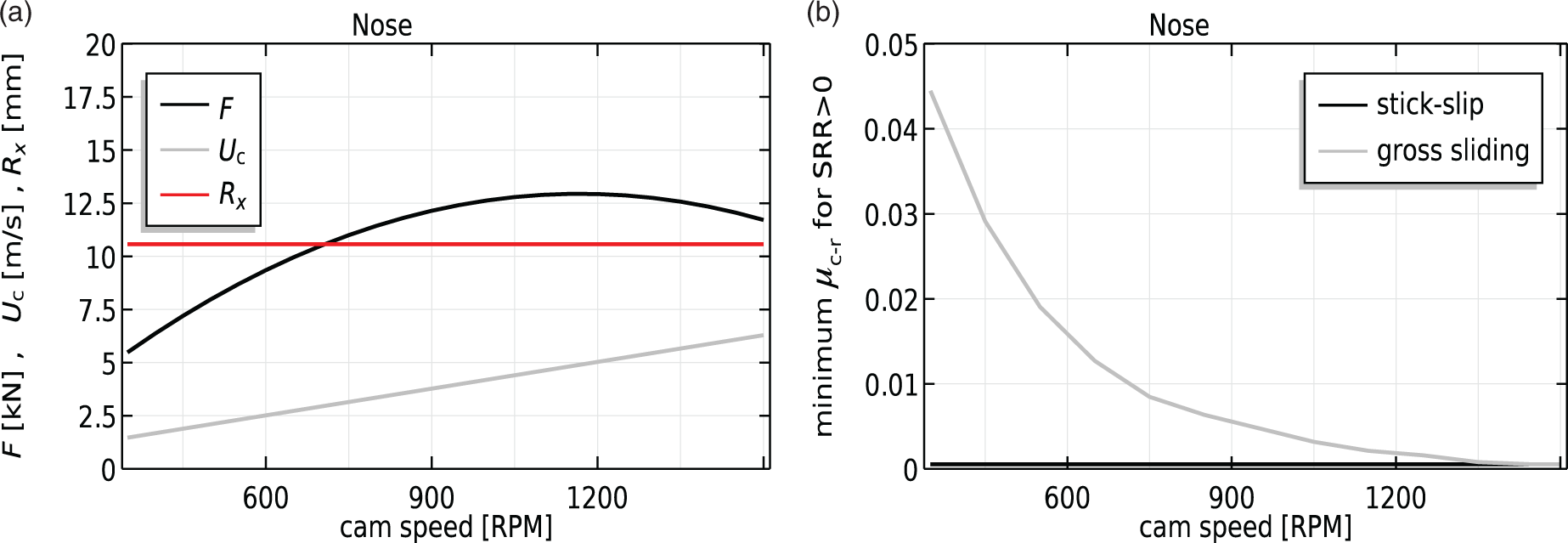

As explained earlier the minimum value of μ_r–p or μ_c–r at which the curve SRR versus μ_c–r starts is defined as to be when SRR > 0. This value of μ_c–r represents the minimum friction coefficient which is required in order to let the cam drive the roller anyway. For a cam rotational velocity of 950 r/min, this was ${\mu }_{\text{c}-\text{r}}=\frac{R_{\text{pin}}{\mu }_{\text{r}-\text{p}}}{R_{\text{f}}}+\frac{I{\stackrel{·}{\omega }}_{\text{r}}}{R_{\text{f}}F}\approx 0.005$ (see Figure 9(a)). In Figure 10(b) the minimum required friction coefficient μ_c–r, in order to drive the roller, is depicted as a function of the cam rotational velocity. Results obtained by assuming a constant asperity friction coefficient (gross sliding) are compared with those considering stick–slip transitions. It is clear from this figure that with decreasing cam rotational speed the discrepancy between the results increases. A decrease in cam rotational velocity comes along with a direct decrease in sum velocity, meaning that the film thickness decreases. This also implies that asperity interaction increases (moving more in to the mixed lubrication regime), so that the contribution of asperity contact friction to the torque balance increases. Assuming a constant asperity friction coefficient thus automatically implies that the overall friction coefficient μ_c–r will increase naturally. Note that the same story, explained earlier, applies here. To be more specific, given a roller–pin friction coefficient μ_r–p and an increase in asperity friction at the cam–roller contact will directly mean a decrease in sliding velocity. Meaning that the minimum required value of μ_c–r so that SRR > 0 will increase, i.e. the minimum required value of μ_c–r so that the cam can actually drive the roller will increase. The aforementioned explains the trend in Figure 10(b) for the gross sliding case.

Note that the procedure for obtaining the minimum value of μ_c–r is similar as was done in the “Parametric sweep: The influence of roller–pin friction” section. In fact from a starting value of μ_r–p = 0.001, μ_r–p is gradually increased with increments of 0.001. The moment a value of μ_r–p is achieved when the condition SRR > 0 holds, the corresponding value of ${\mu }_{\text{c}-\text{r}}=\frac{R_{\text{pin}}{\mu }_{\text{r}-\text{p}}}{R_{\text{f}}}+\frac{I{\stackrel{·}{\omega }}_{\text{r}}}{R_{\text{f}}F}$ is approximated as to be the minimum required friction cam–roller contact friction coefficient in order to let the cam drive the roller.

Taking a look at the curve in Figure 10(b), which accounts for stick–slip transitions, then a huge difference is observed. In fact, the minimum value for μ_c–r ≈ 0.0005 remains constant for the full range of cam rotational velocities considered here. This may be attributed to the fact that for the stick–slip case the asperity friction coefficient has the “ability” to adapt itself, meaning that μ_a basically decreases as the film thickness decreases with decreasing cam rotational velocity. This is in line with the asperity contact friction map (see Figure 7(b)). Note that the contact force also decreases with decreasing cam rotational velocity (see Figure 10(a)); however, the predicted SRRs corresponding to the minimal required μ_c–r (which are not presented here) were still small enough to keep the asperity contact component still in the static friction regime.

Conclusions

In this paper a FEM-based mixed lubrication model, applicable to cam–roller contacts, is developed. Surface roughness effects are efficiently taken into account by making use of the real measured surface topography. In order to calculate the proportion of normal and tangential load carried by the asperities an uncoupled approach was utilized in which precalculated values for the asperity friction coefficient and normal contact pressure, obtained from a BEM-based dry contact stick–slip solver, were used in the macroscopic setting of the mixed lubrication model.

The lubrication performance in a cam–roller follower unit, as part of the fuel injection equipment in heavy-duty diesel engines, was analyzed. The lubrication conditions in two regions of the cam were analyzed, namely specific positions on the base circle and nose region. Results show that stick–slip effects on asperity scale are of crucial importance in regions of the cam where high contact forces occur such as the nose region. Assuming a constant asperity contact friction coefficient (or gross sliding) in these regions may lead to large overestimation in required friction coefficient in order to let the cam actually drive the roller. For the constant asperity friction coefficient case (in the nose region), the overestimation in required cam–roller friction coefficient increases with decreasing cam rotational velocity as the film thickness decreases (and thus the asperity frictional force increases). The importance of including stick–slip transitions into the mixed lubrication model for the cam–roller contact is thus amplified with decreasing cam rotational velocity.

In order to simulate nonlinear viscous behavior of the lubricant in the frictional model, the Eyring friction model was adapted for the sake of simplicity. It was highlighted that for the heavily loaded regions, such as the nose, nonlinear viscous behavior influences the SRR and thus also the stick–slip transitions.

For the base circle regions the acting contact forces are much less when compared to the nose regions. Consequently, the roller slippage is much larger on base circle positions and thus has the inception of gross sliding already occurred. Hence, for base circle regions inclusion of stick–slip effects is negligible. Also, for the considered range of SRRs in this study, nonlinear viscous effects of lubricant in base circle positions are negligible due to the lower pressures which the lubricant experiences.

The focus of this work was on the low SRR domain. At higher levels of friction at the roller–pin contact the SRR will increase indicating that non-Newtonian and thermal effects will become highly important. As such, highly nonlinear effects may occur. Thus, for a more “unified” model (i.e. also valid for the high SRR domain, i.e. high shear rates) more up-to-date rheological formulations (see, for instance Habchi et al. ²³ ) should be used, and also inclusion of non-Newtonian and thermal effects becomes inevitable.