Single-Cell Phenotype Classification Using Deep Convolutional Neural Networks

Abstract

Deep learning methods are currently outperforming traditional state-of-the-art computer vision algorithms in diverse applications and recently even surpassed human performance in object recognition. Here we demonstrate the potential of deep learning methods to high-content screening–based phenotype classification. We trained a deep learning classifier in the form of convolutional neural networks with approximately 40,000 publicly available single-cell images from samples treated with compounds from four classes known to lead to different phenotypes. The input data consisted of multichannel images. The construction of appropriate feature definitions was part of the training and carried out by the convolutional network, without the need for expert knowledge or handcrafted features. We compare our results against the recent state-of-the-art pipeline in which predefined features are extracted from each cell using specialized software and then fed into various machine learning algorithms (support vector machine, Fisher linear discriminant, random forest) for classification. The performance of all classification approaches is evaluated on an untouched test image set with known phenotype classes. Compared to the best reference machine learning algorithm, the misclassification rate is reduced from 8.9% to 6.6%.

Introduction

The cellular composition of organs or tumors is designed by nature to be heterogeneous and complex to fulfill their diverse and complex functions. In the recent past, it has been realized that without taking this cellular heterogeneity into account, model systems for in vitro experiments provide only an oversimplified view of the in vivo situation. To investigate such cellular heterocultures or organoids, detection methods require single-cell resolution as provided, for instance, by imaging mass spectrometry or high-content screening (HCS), where the latter is the method of choice when higher throughput is required. In HCS assays, cellular morphology, protein localization and trafficking, or organelle function is detected by specific markers and fluorescence labels, which define a distinct cellular phenotype.

Discrimination between these different phenotypes is an important task in single-cell image analysis. This is traditionally done in two steps: First, tens or hundreds of image properties (so-called features) are extracted for each cell from the image using specialized software, such as CellProfiler (Broad Institute, Cambridge, MA, USA). ¹ Second, machine learning or statistical models are using these features to train a classification model such as linear discriminant analysis (LDA) or a support vector machine (SVM). In this article, we compare this traditional approach using established machine learning methods against the novel machine learning approach of deep learning.

In general, image-based object recognition is a domain where humans excel over computer algorithms. However, in the past few years, deep learning methods, especially convolutional neural networks (CNNs), have made impressive breakthroughs in image-based classification tasks.^2,3

CNNs are a special kind of artificial neural networks that are inspired by the visual cortex of a human brain, where each individual neuron detects only signals from a small subregion of the visual field, called a receptive field. In analogy, in a CNN, each neuron performs a convolution of a kernel with an input image and produces a filtered output image often called a feature map. The input image can consist of several channels, and each layer in the neural net holds as many channels of feature maps as we have neurons in this particular layer. The feature maps in the last layer can be interpreted as the final features learned by the network and are used for classification. The critical difference from traditional feature-based classification methods is the fact that for CNN, no features, including the weights of the kernels, are predefined, but the algorithm is learning them by itself.

Here we study the potential of the CNN approach for HCS-based phenotype classification. For this purpose, we use a CNN to classify images of individual cells into different phenotypes. We compare the classification rate obtained with CNN with the performance of the best traditional classification approach. Traditional methods require cell features, which have been extracted from the images beforehand, whereas CNN uses the raw image data as input.

Since CNNs learn appropriate features directly from the image data and the attached class labels without external guidelines or predefined feature extraction rules, the CNN approach has the potential to save time and costs during the image analysis step and simultaneously provide better performance and more flexibility compared to traditional approaches.

Materials and Methods

Data Set

We used part of the image set BBBC022v1⁴ (the “Cell Painting” assay), available from the Broad Bioimage Benchmark Collection (Broad Institute, Cambridge, MA, USA). ¹ The images are of U2OS cells treated with 1750 known bioactive compounds and labeled with six labels that characterize the following components: nuclei, nucleoli, actin, endoplasmic reticulum (ER), Golgi, and mitochondria. The images were taken in five channels: DAPI (387/447 nm), GFP (472/520 nm), Cy3 (531/593 nm), Texas Red (562/642 nm), and Cy5 (628/692 nm). Details of the assay and the relevance of the induced phenotypes are described elsewhere^1,4; here we used part of this assay data for benchmarking.

Of the 75 compounds for which chemical information was available, 3 subclasses (clusters A, B, C) with similar mechanisms of action have been defined. ⁴ Cluster A contains modulators of tubulin, here represented by the compounds fenbendazole, oxibendazole, and taxol. Cluster B contains modulators of neuronal receptors, represented by the compounds fluphenazine, metoclopramide, and procaine. Cluster C is enriched for structurally related cardenolide glycosides, represented by the compounds digoxin, lanatoside C, and peruvoside, which are known for significant cytotoxicity, explaining the low numbers of cells (see below). Cluster C thus corresponds to a dead/dying cell phenotype that could probably also be induced by other toxic compounds besides the cardenolide glycosides. To these classes, we added DMSO as the fourth class. In total, we have the following number of detected cells, which were imaged in 21 different wells on 18 different plates: 40783 (DMSO class), 1988 (cluster A), 9765 (cluster B), and 414 (cluster C). Example images for the different clusters are displayed in Supplemental Figure S1.

Approximately 20% of the data were put aside for testing containing data from 8217 (DMSO class), 403 (cluster A), 1888 (cluster B), and 82 (cluster C) cells from 10 different wells on five different plates. The remaining 80% of data were split into a training and a validation set used to train and tune different classifiers comprising CNN based on the raw image data as well as LDA, random forest, and SVM based on CellProfiler features.

To verify the assumption that phenotypes induced by different compounds in the same cluster are comparable and to test the ability of the classifier to predict these phenotypes, we carried out an additional analysis in which we excluded compounds from the training set. Specifically, we used taxol (cluster A), procaine (cluster B), and peruvoside (cluster C) for testing only and excluded those compounds completely from the training set. No DMSO was used in these cases.

The segmentation of the images and the feature extraction were done by using an adapted CellProfiler pipeline provided in the supplementary material. ⁵ The authors kindly provided us with the segmentation information and the extracted features.

For the use of the CNN, for each cell, five images of size (72 × 72) have been cropped from the original images using a bounding box around the cell set up from the CellProfiler features Cell_AreaShape_Center_X,Y, Cell_AreaShape_MajorAxisLength, Cell_AreaShape_MinorAxisLength, and Cell_AreaShape_Orientation. The bounding box was constructed to be quadratic so that the entire cell was within the box. Cells with a bounding box not completely inside the image field were excluded from further analysis. The workflow is sketched in Figure 1 .

Figure 1.

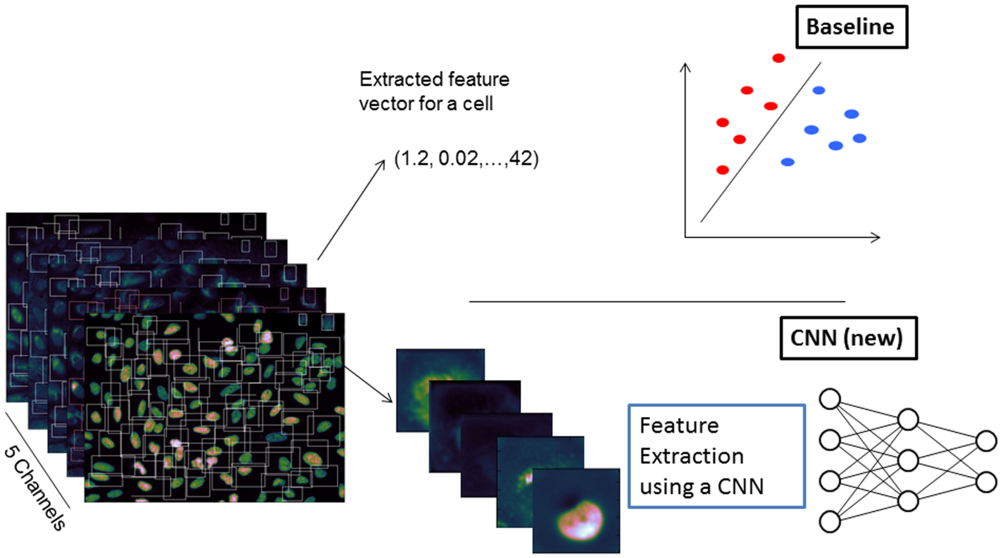
Overview of the used analysis scheme. The baseline approach (upper part) needs handcrafted features, which are extracted using CellProfiler prior to classification such as support vector machine. In the convolutional neural network (CNN) approach (lower part), the features are learned as well.

Baseline workflows

For the baseline workflows, we normalized each of the extracted features to zero mean by a z-transformation.

We used the following algorithms for the baseline approach: a SVM with a linear kernel (the penalty parameter C of the SVM was optimized using a 10-fold cross-validation on the training set), a random forest with 500 trees, and a Fisher LDA. We used python implementations provided in the scikit library ⁶ for all of these algorithms.

CNN

As the only preprocessing step for CNN, we normalized the values per pixel position with the same z-transformation calculated for each pixel at the same image position in the training set. The architecture of our CNN was inspired by a design by Simonyan and Zisserman. ⁷ All convolutional layers (C) had several kernels each with the size of (3,3) and accordingly nine weights. The convolution of a kernel with a patch of the image was followed by a rectified linear transformation ⁸ and repeated after shifting the kernel with a stride of 1 pixel; no padding was applied at the boundaries. The feature learning part of the network was constructed by three stacks. In each stack, two convolutional layers were followed by a (2,2) max-pooling layer, which performed downsampling of the feature maps by the factor of 2. In our implementation, the convolutional layers in the stacks had 32, 64, and 128 kernels. The stacks were followed by three fully connected layers with 200, 200, and 50 nodes, respectively, and a final softmax layer for the four classes. The network has about 1.2 million learnable weights, including the weights of the kernels in the convolutional layers, and is summarized in Table 1 . For learning the weights of the network, we split the data available for learning into two parts; one part was used for fitting the weights (training set), and the other 20% were used for validation (validation set). Note that the test set was used only for the evaluation of the trained CNN.

Table 1.

Architecture of the Convolutional Neural Network.

Layer Description	No. of Images/Feature Maps × Their Dimensions	No. of Weights
Input	5 × 72 × 72
Convolution (3 × 3)	32 × 70 × 70	32 × 9 × 5
Convolution (3 × 3)	32 × 68 × 68	32 × 9 × 32
Max pooling (2 × 2)	32 × 34 × 34
Convolution (3 × 3)	64 × 32 × 32	64 × 9 × 32
Convolution (3 × 3)	64 × 30 × 30	64 × 9 × 64
Max pooling (2 × 2)	64 × 15 × 15
Convolution (3 × 3)	128 × 13 × 13	128 × 9 × 64
Convolution (33)	128 × 11 × 11	128 × 9 × 128
Max pooling (2 × 2)	128 × 6 × 6
Fully connected	200	200 × 128 × 6 × 6
Fully connected	200	200 × 200
Fully connected	50	50 × 200
Output	4	4 × 50

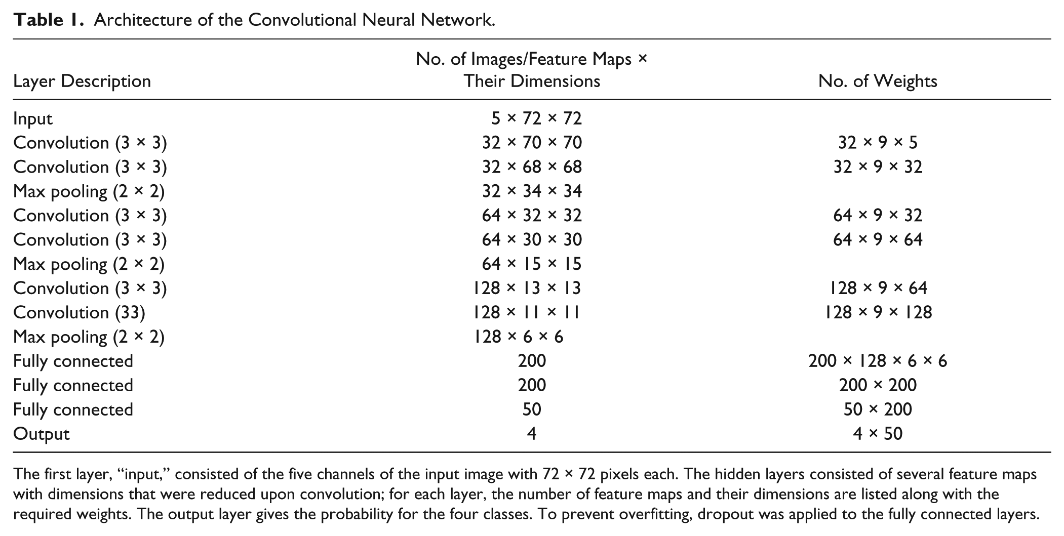
The first layer, “input,” consisted of the five channels of the input image with 72 × 72 pixels each. The hidden layers consisted of several feature maps with dimensions that were reduced upon convolution; for each layer, the number of feature maps and their dimensions are listed along with the required weights. The output layer gives the probability for the four classes. To prevent overfitting, dropout was applied to the fully connected layers.

Due to the large numbers of parameters, CNNs are prone to overfitting. We used dropout ⁹ for the hidden layers during the training phase to prevent overfitting, setting 30% of all nodes randomly to zero in optimization step. We further virtually enlarged the training set by applying the following random transformations to each image after each epoch (full pass through the training set): a random rotation uniformly chosen in the range of 0 to 360 degrees, a random translation up to 5 pixels in each direction (uniformly chosen), and scaling by a factor uniformly in the range between 0.9 and 1.1. In a CNN, these augmented data constitute additional samples, facilitating efficient learning of translational and rotational invariant features. These invariances are usually already taken into account in the predefined features as used in traditional methods, which therefore would not benefit from this kind of data augmentation.

The network was implemented using the nolearn extension of the lasagne python library. ¹⁰ To optimize the weights in the CNN, we used stochastic gradient descent with an initial learning rate of 0.01 and a Nestrov momentum set to 0.9 to avoid oscillations of the parameter updates, which were determined with respect to the results on a mini-batch of 256 images. All runs were done on an off-the-shelf PC with a NVIDIA GeForce GTX 780 GPU with CUDA 6.0 installed running on a Debian 7.5 (Santa Clara, CA, USA).

Results and Discussion

We mimicked the traditional HCS data analysis workflow using predefined features extracted from cell images to train a machine learning method of the analyst’s preference. A comparative study of classifier performance in HCS ¹¹ suggested to use SVM for phenotype classification. In our study, we have used SVM, LDA, and random forest as three of the most prominent and successful classification methods on features that have been extracted from experts of the field.

Baseline

We found that the performance of the SVM is best when not using all training data from the largest group (DMSO) but limiting them to the same size as the next largest group (cluster B) in the training set. No such effect was found for the other baseline classifiers, and thus they were trained on the whole training set. Furthermore, for the SVM, the parameter C was optimized using the training set resulting in C = 0.01. No parameter optimization was needed for the LDA and the random forest. We obtained the following results for the accuracy on the hold-out test set: SVM, 87.6%; LDA, 91.1%; and random forest, 89.2%. The result for the SVM (87.6%) is in accordance with the accuracy of 88.4% reported for the same data set on a stratified test set. ⁵ The confusion matrix of the best baseline approach (LDA) is shown in Table 2 .

Table 2.

Confusion Matrix for the CNN and the LDA.

	DMSO (True)	Cluster A (True)	Cluster B (True)	Cluster C (True)
CNN
DMSO	7775	13	208	0
Cluster A	28	382	23	1
Cluster B	414	8	1657	0
Cluster C	0	0	0	81
LDA
DMSO	7949	20	542	0
Cluster A	15	323	35	12
Cluster B	251	60	1310	1
Cluster C	2	0	1	69

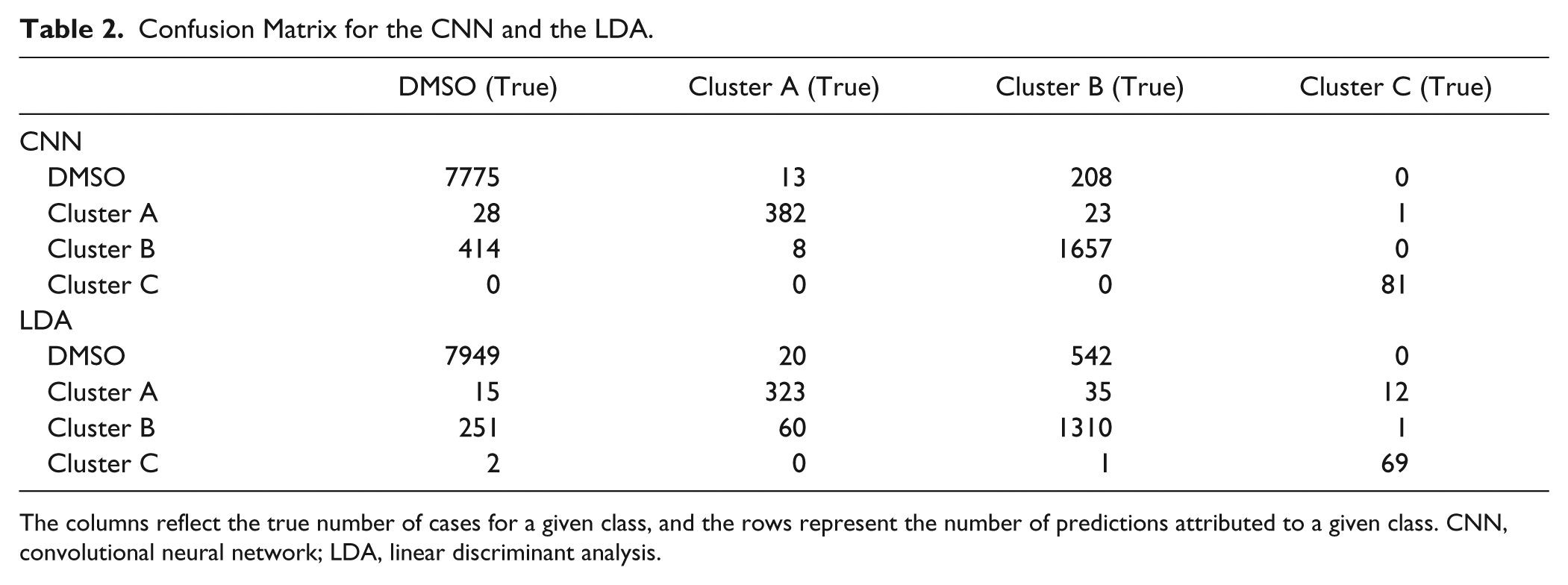
The columns reflect the true number of cases for a given class, and the rows represent the number of predictions attributed to a given class. CNN, convolutional neural network; LDA, linear discriminant analysis.

In an additional analysis, we excluded for each of the clusters A, B, and C one compound from the training data and used them to test the performance of the trained CNN based on the fact that phenotypes A, B, or C should be predicted. The following accuracies have been obtained: SVM, 88.6%; LDA, 94.6%; and random forest, 90.2%. Since no DMSO is classified in this case, the accuracies are generally higher. These results support the assumption that the compounds in the same clusters have similar phenotypes.

In contrast to the authors of the comparative study, ¹¹ we found that LDA yields the highest accuracy in both analyses.

Convolutional Neural Net

The training of the CNN took on average 135 s per epoch when using augmentation of the training data; without augmentation, an epoch took just 70 s. The network was trained for 512 epochs; the performance parameters log-loss and classification accuracy for the validation set are shown in the lower part of Figure 2 . For comparison, we also ran a network for 100 epochs without augmentation (see left side of Fig. 2 ).

Figure 2.

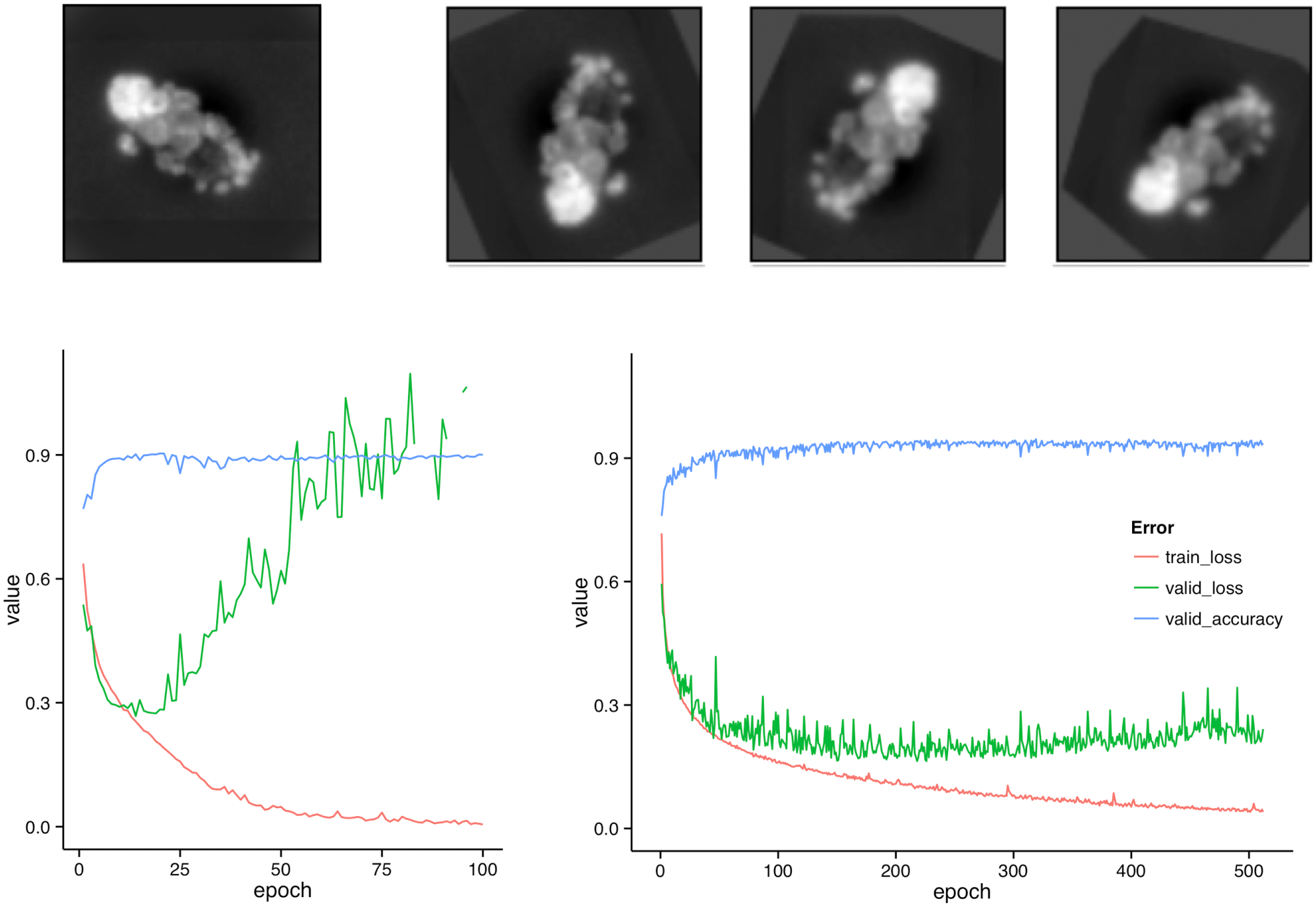
Augmentation and its benefit. The upper half of the figure shows the data augmentation step: the original image of a cell (left) and three random transformations of the same cell (right) are the first channel (DAPI). If no augmentation is done, overfitting is observable after approximately 20 iterations (bottom, left). With augmentation, the training set is effectively enlarged, and no pronounced overfitting is visible after 500 epochs (bottom, right).

Without augmentation, we were in an overfitting regime after about 20 epochs, where the training loss continued to decrease but the validation loss and the accuracy on the validation set began to deteriorate. With augmentation, we avoided overfitting, and the validation accuracy was still at its maximum value after 512. Averaged over the final 100 epochs, the validation accuracy was on average 0.9313 (SD, 0.0079).

The trained network was then applied to the test set consisting of 10,590 cell images. In contrast to the long training phase, the prediction of the probabilities for the four classes only took approximately 6.9 s for all images. The overall accuracy was 93.4%. The confusion matrix is shown in Table 2 together with the best baseline approach (LDA).

In an additional analysis, we excluded for each of the clusters A, B, and C one compound from the training data and used them as test data. Here the CNN misclassified 60 of the 2223 cells in the test set, corresponding to a performance of 97.3%. This demonstrates the ability to correctly classify phenotypes of compounds not seen in the training phase. The 60 incorrectly predicted cells are shown in the supplementary materials. In conclusion, the CNN trained with raw images yields the best classification accuracy in this HCS data analysis study compared to three state-of-the-art classifiers trained with previously extracted cell features. However, on this rather simple data set, all approaches reached a relatively high performance. It will be interesting to see CNNs outperform traditional approaches where they fail to reach acceptable accuracy.

While the training of a CNN is quite time-consuming, the classification of new data with a trained CNN model is very fast and can be done on a simple laptop. Since no extra feature extraction step is needed, it is faster than phenotype classification with traditional approaches. A trained CNN can easily classify more than 1000 cells per second.

There is a trend in image classification to use pretrained CNN models to speed up the training time. The pretraining is done with more general images, which might come from outside the direct classification task domain. We are convinced that this approach is also promising for the HCS field when a fast training is required or the amount of training data is limited.

To our knowledge, we have for the first time demonstrated the use of CNNs for phenotype classification in HCS. We believe that this can trigger valuable stimuli in the HCS community. Besides the high accuracy of the CNN approach, the self-learned hierarchical features can offer additional benefits since these features are unbiased and might provide new insights into crucial structures for the discrimination of classes. Moreover, no image analysis expert knowledge is required for feature generation, which can lead to a considerable saving of time and resources during the development phase.