
Abstract
High-content screening is a powerful method to discover new drugs and carry out basic biological research. Increasingly, high-content screens have come to rely on supervised machine learning (SML) to perform automatic phenotypic classification as an essential step of the analysis. However, this comes at a cost, namely, the labeled examples required to train the predictive model. Classification performance increases with the number of labeled examples, and because labeling examples demands time from an expert, the training process represents a significant time investment. Active learning strategies attempt to overcome this bottleneck by presenting the most relevant examples to the annotator, thereby achieving high accuracy while minimizing the cost of obtaining labeled data. In this article, we investigate the impact of active learning on single-cell–based phenotype recognition, using data from three large-scale RNA interference high-content screens representing diverse phenotypic profiling problems. We consider several combinations of active learning strategies and popular SML methods. Our results show that active learning significantly reduces the time cost and can be used to reveal the same phenotypic targets identified using SML. We also identify combinations of active learning strategies and SML methods which perform better than others on the phenotypic profiling problems we studied.
Keywords
Introduction
Developments in fluorescence labeling, automation, microscopy, data storage, and image analysis have paved the way for a new era of biological research using high-content screening (HCS). In a high-content screen, vast quantities of biological data are collected and analyzed to identify small molecules, peptides, or genes that alter the phenotype of a cell. HCS is used extensively by the pharmaceutical industry throughout all stages of the drug development process. 1 It has also emerged as a powerful approach for defining protein functions and understanding signaling pathways among academic investigators, thanks in large part to recent advances in genome-wide RNA interference (RNAi) technology. 2
High-content screens capture a compound’s molecular and phenotypic effects on a cell through a wealth of extracted image data. In traditional high-throughput screening methods, biological responses from thousands of cells are aggregated into a few carefully selected project-specific readout parameters. In contrast, high-content screens use image analysis to extract functional and morphometric data from individual cells on a massive scale. In the course of a typical genome-wide RNAi screen, researchers acquire millions of images and then extract and store abundant quantitative information to characterize the cells, such as intensity, size, morphology, spatial distribution, and texture for computational analysis. With so much data, the search for positive results, or “hits,” can be daunting. Early approaches to hit identification ranked all compounds by a single parameter; those above a statistically determined threshold were considered hits. 3 Filtering with additional parameters can improve the process but does not address the principal drawbacks of this approach: the difficulty of identifying which combinations of parameters are useful, human bias in choosing which parameters determine the hits, and the failure to exploit all of the information acquired from the image analysis.
Supervised machine learning (SML) has helped to address this problem by simultaneously considering all the parameters collected during image analysis and automatically sorting compounds according to predicted hit quality.4,5 Recent studies have shown that SML methods identify target compounds with significantly more reliability than manual parameter selection. 6 SML also eliminates human bias introduced during parameter selection by considering every parameter for its prediction. As SML methods have become more widely used in high-content screen analysis,7,8 they have demonstrated the power of multiparametric readouts to distinguish between true biological activity and nonbiological interference.
With machine learning, a new bottleneck has arisen in the analysis stage of the HCS process. Even without machine learning, experimenters face the arduous task of manually sifting through oceans of data in search of the right combination of parameters to generate a valid hit list. But if SML is used for hit identification, experimenters must provide the algorithms with labeled examples to build a predictive model in what is known as the training process. Typically, several hundred to several thousand examples are necessary for the classifier to achieve satisfactory performance, and providing more examples nearly always increases performance, although at a diminishing rate. Depending on the difficulty of the problem, labeling an individual cell can take on average between 3 and 15 s; therefore, the annotation process represents a significant time investment. Fatigue further complicates the issue: because annotation quality degrades over time, the biologist is often forced to perform the labeling in multiple sittings.
In a typical annotation setting, the expert, or “oracle,” is presented with an image from the high-content screen chosen at random. The expert then decides which of the cells that appear in the image to label, evaluates them, and assigns the appropriate labels. To speed up the process, some practitioners use a classifier trained on data from previously annotated images to make predictions for every cell in a new image, and the expert is asked to correct the predictions. In the first case, human selection bias means that the labeled population is often highly correlated and not representative of the true population. But it is more concerning that both schemes unintentionally waste the expert’s effort. A significant amount of time will be spent unknowingly labeling hundreds or even thousands of cells that have little impact on the decision boundary of the learning algorithm. Recently, active learning strategies have emerged as a way to improve classification performance using less training data, thereby making more efficient use of the expert’s valuable time. They do so by allowing the learning algorithm to select the data it uses to learn through relevant queries posed to the expert.
This article explores how active learning strategies can be leveraged to make more efficient use of the expert’s time, achieving high hit identification accuracy while minimizing the cost of obtaining labeled data. In particular, we compare four well-known active learning strategies and six popular machine learning algorithms on data taken from three large-scale RNAi high-content screens representing a diverse set of phenotypic profiling problems. Our investigation measures performance over time using implementations from the popular software packages Advanced Cell Classifier 8 and Weka. 9 In addition, we provide a software-agnostic evaluation measuring classification performance for every query posed to the expert. Our results show that for the HCS assays we consider, there always exists an active learning strategy that will significantly increase the rate at which the classifier learns. In some cases, the time can be reduced by over a factor of 3. Although no one active learning strategy consistently ranked the best, some performed consistently better than others. And interestingly, a few strategies actually perform worse than passive learning if training time is taken into account.
Materials and Methods
Ribosome Biogenesis Assay
The biosynthesis of proteins in cells is performed by ribosomes, macromolecular complexes that consist of a large (60S) and a small (40S) subunit. In eukaryotes, the production of ribosomes is a complex, highly compartmentalized process that begins in the nucleolus. Both ribosomal subunits undergo separate maturation in the nucleolus and nucleoplasm before they are exported to the cytoplasm where final maturation occurs. Both subunits join to form the translational competent machinery. 10 To investigate 40S biogenesis, a tet-inducible RPS2-YFP (40S) HeLa cell line was generated that allows us to observe the nuclear maturation of freshly synthesized precursors of the small ribosomal subunit. This image-based assay partially relies on RPS2-YFP localization as readout. Under normal biogenesis conditions, the reporter mainly localizes to the cytoplasm, reflecting mature ribosomes. If biogenesis defects occur either in the nucleolus or the nucleoplasm, the reporter localizes to the respective cellular compartment and the cytoplasmic signal is strongly reduced. 11 This assay was used in a genome-wide RNAi association study using the Qiagen Human genome-wide siRNA library (HsNmV1; Qiagen, Venlo, the Netherlands) and analyzed using HCS. Example images are provided in Figure 1a .
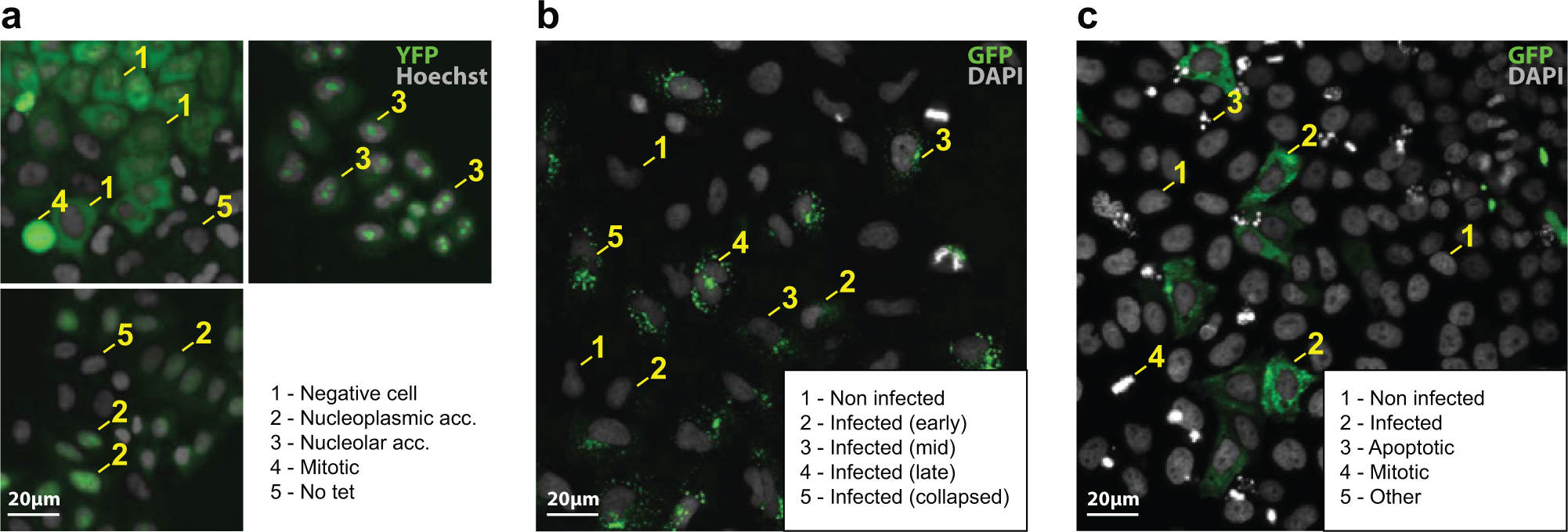
Examples images from the high-content assays considered in this study: (
Semliki Forest Virus Assay
Semliki Forest virus (SFV) is an alphavirus (Togaviridae) transmitted by mosquitoes.
12
In humans and animals, it can cause serious diseases including long-lasting arthritis and lethal encephalitis. This virus replicates very efficiently in most cell culture systems, completing its life cycle in few hours. Here we used a recombinant SFV that was genetically engineered to expresses a green fluorescent protein.
13
Soon after infection, the viral RNA genome is delivered in the cytoplasm of the cell. Here the ribosomes, cellular machineries responsible for the production of proteins, start to produce the viral proteins. One of these viral proteins was fused with green fluorescent protein. At the beginning of infection, a few small green spots appear in the cell. As the infection proceeds and more viral proteins are produced, these fluorescent spots become larger, brighter, and concentrate around the nucleus of the cell. Thus, by monitoring the intensity distribution and texture of the green fluorescence, it is possible to distinguish between the different stages of infection, as well as noninfected cells. This assay was used in a genome-wide RNAi association study using the Dharmacon Human genome-wide siRNA library and analyzed using HCS. Example images from the screen are provided in
Figure 1b
(corresponding segmentations appear in
Uukuniemi Virus Assay
Uukuniemi virus (UUKV) belongs to the virus family of Bunyaviridae that contains more than 350 segmented,negative-stranded RNA viruses. 14 As a nonpathogenic virus for humans, UUKV serves as a model for some severe human pathogenic bunyaviruses such as the Rift Valley fever virus. 15 To study the host genes that are involved during the entry steps of UUKV, we conducted a genome-wide siRNA screen using the Qiagen Human genome-wide siRNA library. To monitor infected cells, we used indirect immunofluorescence against the viral nucleoprotein that is expressed in newly infected cells. After bunyaviruses enter into their host cells, their genome is released into the cytoplasm where the replication and the production of new viral proteins occur. Thus, we were able to classify infected and uninfected cells after depletion of a gene. Example images from the screen are provided in Figure 1c .
Microscopy
Images were acquired using two Molecular Devices (Sunnyvale, CA) ImageXpress Micro microscopes equipped with an automated plate loader and with 10x S Fluor 0.45NA objectives. The automated microscopes acquired nine sites per well arranged in a 3 × 3 slightly overlapping grid. Laser-based autofocusing was used to ensure that images were focused at every site. Two fluorescent channels were recorded for each high-content screen. For the ribosome biogenesis assay, a Hoechst channel was used for nuclear staining, and a YFP reporter is bound to the 40S subunit. For the SFV assay, a DAPI channel was used for nuclear staining, and a GFP channel reports the stage of viral infection. For the UUKV assay, a DAPI channel was used for nuclear staining, and a GFP channel was used to indicate if a cell was infected.
Image Analysis
The software analysis package CellProfiler
16
was used to segment individual cells and extract features from images acquired for each screen. Several custom modules were used to increase the speed of the analysis. The image analysis for all three assays followed a common framework. First, the cellular nuclei were detected and segmented using Otsu adaptive thresholding and the watershed algorithm on the DAPI/Hoechst channel. Next, the nuclei were used as “seed” regions, and the cytoplasm is approximated as a ring surrounding the nucleus. From these regions denoting cellular compartments, various features were extracted for each cell describing the intensity, morphology, and texture. For the ribosome biogenesis assay, 26 features were collected, mostly intensity-based (eg, integrated intensity, mean intensity of the nucleus/cytoplasm, standard deviation of intensity of the nucleus/cytoplasm, intensity along the edge of the nucleus, etc.). Texture features were also collected to describe the contrast, correlation, variance, entropy, gradient, and so forth. The UUKV assay used the same features as the ribosome biogenesis assay, with two additional features describing the nucleus intensity, for a total of 28 features. A total of 94 features were collected for the SFV assay. In addition to the features described above, several morphological features were collected such as area, perimeter, form factor, eccentricity, and so on. A full list of the extracted features is given in
Multiparametric Analysis Using SML
With so many features available in a high-content screen, it is too difficult to take every feature into account while manually performing hit identification. Although early works restricted themselves to just a few interpretable features, researchers have turned to machine learning to consider all the features collected during the image analysis. A few studies have made use of unsupervised learning techniques such as clustering 18 and self-organizing maps, 19 but the majority have opted for supervised techniques.4,5,7,8 SML infers a mapping function from labeled training data, which consists of a set of training example pairs (a feature vector describing the cell and the desired class label). The supervised learning algorithm uses the training data to produce a function that maps unseen instances to the desired output. This requires the supervised learning algorithm to generalize to unseen situations in a reasonable way.
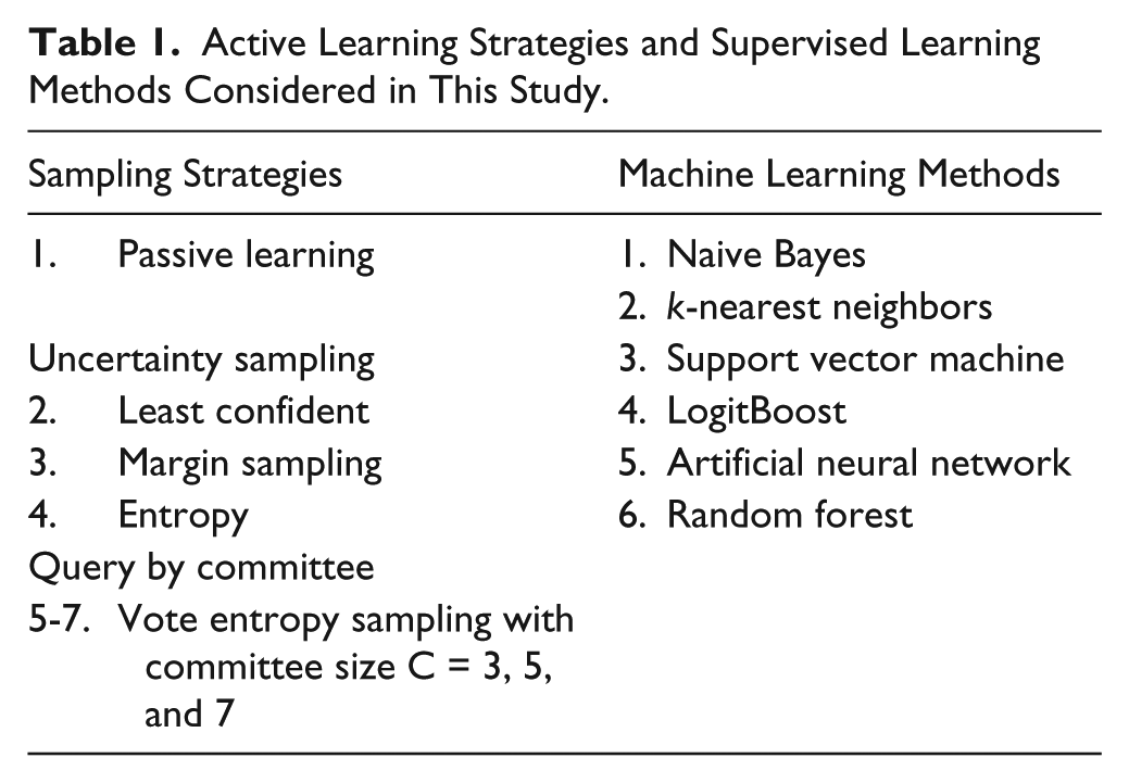
In this study, we consider six popular SML methods: Naive Bayes, KNN, SVM, LogitBoost, ANN, and random forest. The first, Naive Bayes, builds a prior probability of the class distribution and uses Bayes rule to update this using kernel density estimates from features of other examples. It is well suited for high-dimensional feature vectors and, despite its simplicity, can outperform more sophisticated methods. The second, k-nearest neighbors, or KNN, is a nonparametric instance-based learning method that predicts class membership based on the k closest training examples. KNN can be a powerful predictive model, but the training process does not scale well for large data sets. A support vector machine, or SVM, is a method for finding the best separating hyperplane for linearly separable problems. It can be extended to nonlinearly separable problems through the use of kernel functions and is one of the most popular and dependable machine learning methods. LogitBoost is an adaptation of AdaBoost set in a statistical framework that minimizes logistic loss on decision stumps. Adaboost is a meta-algorithm that trains a series of simple classifiers, each tuned to correct for mistakes made by the previous classifiers. It can be a powerful predictor for difficult problems. Artificial neural networks, or ANNs, are networks of artificial neurons that map several weighted inputs to a desired output, inspired by neurons in the brain. Random forests train thousands of decision trees on randomly chosen subsets of the feature space and make predictions by running the new instance to the terminal node of all the trees and performing some statistical measurement. For this study, we used the WEKA 9 implementations of the above machine learning methods with parameters selected for the best performance using an extensive cross-validated random search. A summary of the supervised learning methods considered in this study is provided in Table 1 .
Active Learning Strategies and Supervised Learning Methods Considered in This Study.
The standard procedure for collecting the labeled data necessary for the SML method to learn the mapping function is sometimes referred to as passive learning. The expert is presented with a set of instances randomly sampled from the data and is asked to assign labels to each. Alternatively, the expert is allowed to choose which samples to label. In this study, an instance corresponds to an individual cell, the labels are nominal, and the expert is provided with an image selected at random and allowed to choose which cells to annotate. The resulting set of labeled instances, called the training set, is supplied to the algorithm for learning, or model training. SML algorithms require a large training set to perform well, and prediction accuracy increases as the size of the training set increases. The labeling process is strenuous and must usually be broken into multiple sittings to ensure fatigue does not compromise the quality of the data. These factors constitute a significant time investment from the experts, making the passive learning process a major bottleneck in HCS.
Active Learning Strategies
Passive learning does not make efficient use of the expert’s time. There is no guarantee on the usefulness of the labels provided by the expert, regardless of whether the expert chose the cells to label or if they were selected at random. To help eliminate this bottleneck, we consider several active learning strategies to make more efficient use of the expert’s time. Active learning is an iterative process that aims to minimize the cost of obtaining labeled data by carefully selecting the most informative examples for labeling. Consequently, active learning strategies promise to produce a more accurate predictor in significantly less time than passive learning.
Active learning can be broadly categorized into three frameworks: pool-based sampling, stream-based sampling, and membership query synthesis. Pool-based sampling is appropriate when large collections of unlabeled data can be gathered all at once. In pool-based sampling, there exists a large pool of unlabeled data U and a small set of labeled data L. Unlabeled samples are selectively drawn from the unlabeled pool according to an informativeness measure and presented to the oracle (expert) for labeling. 20 This process is referred to as a query. It is common to repeat this in an iterative cycle, as depicted in Figure 2 . An instance or set of instances is sampled from the unlabeled pool using some selection strategy and presented as queries to the oracle. The oracle uses expert knowledge to provide labels, and then the instance(s) are added to the labeled data. Next, the predictive model is retrained with the updated labeled data. After retraining, the SML algorithm makes predictions on the unlabeled pool, which are used by the selection strategy to measure the informativeness of each instance when choosing the next query. In this way, the cycle iteratively improves classification performance by querying the expert with the most useful unlabeled example(s) and retraining the model.
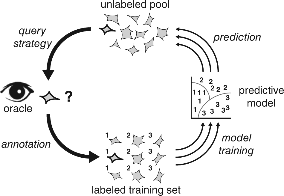
The active learning cycle. Starting from the top, an instance or set of instances is sampled from the unlabeled pool using a query strategy and presented as queries to the oracle (expert). Using expert knowledge, the oracle provides labels to the queries, and then the labeled instance(s) are added to the labeled training set. The labeled training set is a collection of all previously annotated labeled instances. Next, the predictive model is retrained with the updated labeled training data. After retraining, the SML algorithm makes predictions for each instance in the unlabeled pool (or a subset of it), which are then used by the query strategy to measure the informativeness of each instance when choosing the next query. In this way, the cycle iteratively improves classification performance by querying the expert with the most useful unlabeled example(s) and retraining the model.
For high-content screens, pool-based sampling is typically the most appropriate framework because the assay and image analysis provide an extremely large pool of unlabeled data. But it is worthwhile to explain briefly the other frameworks, as some situations may arise in which they are also useful. Stream-based sampling is used when instances are drawn one at a time from the data source; real-time stock market data are a good example. In this case, the task of the active learning is to decide whether to query the oracle or discard the data, based on the expected usefulness. 21 In the membership query synthesis framework, the oracle is presented with either real examples or synthetically generated examples from the input space. 22 Although this approach is not immediately useful for high-content screens, progress in the creation of valid cellular generative models means that it might one day be practical.
All active learning methods must evaluate the informativeness of unlabeled instances and choose which instances to present to the oracle. How this problem is formulated is known as the query strategy. Many query strategies exist in the literature. Expected model change attempts to estimate which instance would impart the greatest change to the current model if its label were known. 23 Expected error reduction attempts to measure not how much the model is likely to change but how much its generalization error is likely to be reduced. 24 Similarly, expected variance reduction attempts to indirectly reduce generalization error by minimizing the variance of the output. In this work, we focus on the two most popular query strategies: uncertainty sampling and query by committee.
Uncertainty Sampling
The simplest query strategy, uncertainty sampling, attempts to select instances about which it is the least certain how to label. For probabilistic SML methods, it is straightforward to use the predicted class probabilities to measure uncertainty directly. One method is to query the instance whose prediction is the least confident, 25
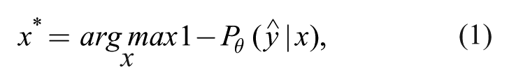
where
To correct for this, some researchers use a query strategy that considers the first and second most probable class label, known as margin sampling, 26 in which the most informative instance is given by
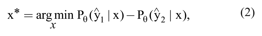
where
Margin sampling still considers only the two most probable class labels. A more general query strategy that considers all predicted class labels uses the entropy as a measure of uncertainty, 27
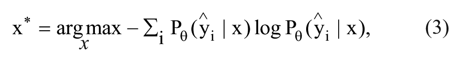
where
Query by Committee
A more theoretically motivated query strategy first proposed by Seung et al.,
28
query by committee, constructs a “committee” of models
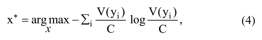
where
Table 1
summarizes the active learning strategies considered in this study. In total, we compare seven different strategies including passive learning, three variants of uncertainty sampling, and three variants of query by committee. Query by committee using vote entropy is tested for three, five, and seven committee members. In all cases, committee members are trained using instances sampled with replacement from the labeled training set L, where
Data Sets
We collected an expert-labeled data set for each of the assays described above. A summary is provided in
For the ribosome biogenesis assay, cells belong to one of the following classes. Examples of each class appear in Figure 1a .
Negative: No biogenesis defect in the cell; the reporter is localized in the cytoplasm
Nucleoplasmic accumulation: A biogenesis defect occurred in the cell; the reporter is localized in the nucleoplasm
Nucleolar accumulation: A biogenesis defect occurred in the cell; the reporter is localized in the nucleoli
Mitotic: The cell is undergoing mitosis
No tet: The reporter failed to activate in this cell
For the SFV assay, cells belong to one of the following classes. Examples of each class appear in Figure 1b .
Noninfected: No reporter presence indicates that the cell is not infected
Infected (early): A few faint localized reporters indicate early stage of infection
Infected (mid): More numerous, larger reporters indicate mid stage of infection
Infected (late): Larger, brighter reporters (sometimes clustered) indicate the late stage of infection
Infected (collapsed): Clustered, bright reporters accompany a dramatic change in cell morphology after cell collapse.
For the UUKV assay, cells belong to one of the following classes. Examples of each class appear in Figure 1c .
Noninfected: No reporter presence indicates that the cell is not infected
Infected: The presence of the viral nucleoprotein causes the marker to be expressed in the cytoplasm
Apoptotic: Fragmented morphology of the nucleus indicates programmed cell death
Mitotic: The cell is undergoing mitosis
Other: Used to collect cells that occasionally encountered image segmentation problems.
Performance Evaluation
The efficiency of an active learning strategy is typically measured by computing the accuracy of the classifier after every query. By plotting the accuracy against the query index, we can generate a learning curve (depicted in Fig. 3 ), and integrating the area under the learning curve (AUC) provides a useful measure of how quickly the active learning strategy improves classifier performance. 26 However, measuring performance this way neglects an important practical component of the evaluation, namely, the time cost to the expert. Labeling a cell and retraining the classifier requires time and effort from the expert, and this fact should be accounted for in the performance evaluation. It may well be that an active learning strategy that appears to be more efficient when measured per query is actually inefficient when we consider how much time it took to label and train.
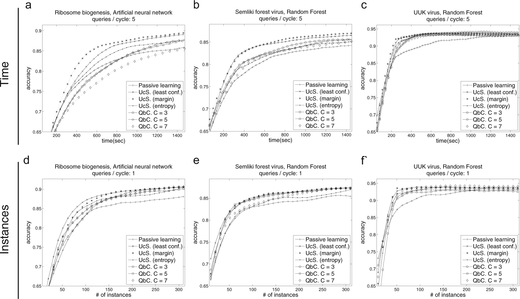
Learning curves for various active learning strategies. The top row shows learning curves as accuracy versus time, and the bottom row shows the accuracy versus number of instances. The curves shown here were selected based on the highest mean area under the learning curve. A complete set is provided in
Therefore, to provide a more practical measure of learning efficiency, we measure the performance of an active learning strategy by computing the AUC over time instead of per query. This provides a better measurement of whether we have achieved our ultimate goal of reduced training and annotation time, but it comes with a caveat. The annotation time and model training time are linked to the data, the software, and the machines used for testing. Thus, the time measurements we report are specific to the problems considered in this study, although we made an effort to choose representative assays and popular implementations of SML methods.
Because our evaluation considers the time needed to retrain the SML model, a new question arises: what is the most efficient number of queries to present to the expert before retraining the SML model and proceeding with the next iteration of the active learning cycle? To answer this, we also run tests to investigate what is the optimal number of queries per cycle for each combination of active learning strategies and SML methods on all the HCS assays.
Results and Discussion
We tested 42 combinations of SML methods and active learning strategies (six supervised learners and six active learning strategies, plus passive learning). Each combination was evaluated for
A summary of the results is provided in
Figure 4
(results reported in
Fig. 4
use three queries per cycle). Each column represents a combination of an active learning strategy and SML method, grouped by SML methods. The first three rows show results for the three high-content screens, and the last row shows the average of the three. The number above each bar graph is the average normalized AUC measured over time. Passive learning performance is indicated by a white bar, and the best active learning strategy for each SML method is indicated by a dark bar. The overall best performing strategy for each high-content screen is indicated by an asterisk. A similar table is provided in
Figure 5
(results reported in
Fig. 5
use one query per cycle), but the scores are measured per instance instead of over time. The average labeling time for each data set is provided in
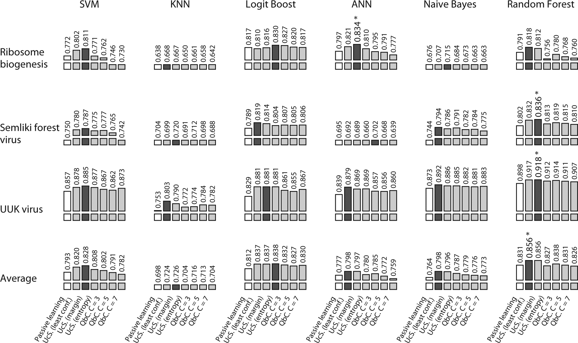
Summary of active learning strategy efficiency (based on time). Performance is measured using the normalized area under the learning curve (AUC) over time. Each column represents a combination of an active learning strategy and supervised machine learning (SML) method, grouped by SML method. The first three rows show results for the three high-content screens, and the last row shows the average of the three. The number above each graph is the average AUC over five tests. Passive learning performance is indicated by a white bar, and the best active learning strategy for each SML method is indicated by a dark bar. The overall best performing strategy for each high-content screen is indicated by an asterisk.
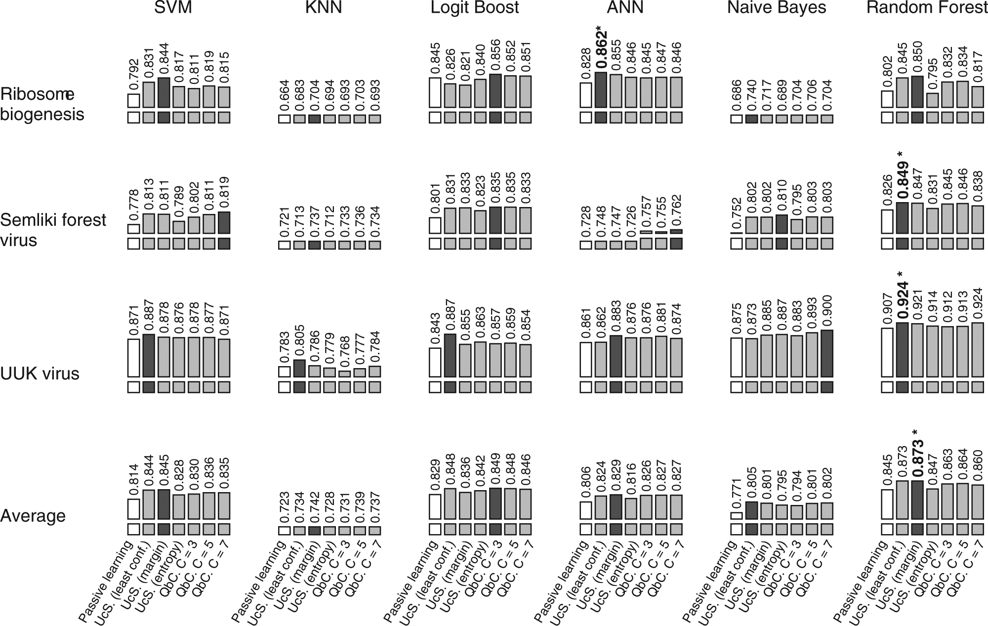
Summary of active learning strategy efficiency (based on queries). Performance is measured using the normalized area under the learning curve (AUC) per query. Each column represents a combination of an active learning strategy and supervised machine learning (SML) method, grouped by SML method. The first three rows show results for the three high-content screens, and the last row shows the average of the three. The number above each graph is the average AUC over five tests. Passive learning performance is indicated by a white bar, and the best active learning strategy for each SML method is indicated by a dark bar. The overall best performing strategy for each high-content screen is indicated by an asterisk.
Learning curves for each high-content screen are shown in Figure 3a–c. In each case, the most efficient active learning strategy and SML method combination are provided, along with other active learning strategies for the same SML method. Similar curves are provided in Figure 3d–f measured per instance instead of over time. A complete set of learning curves is provided in
In
Overall Performance
The results appearing in Figure 4 indicate that for the three phenotypic profiling problems considered in this study, there always exists an active learning strategy that will speed up the annotation process. However, there is no universally most efficient combination of active learning strategy and SML method. Random forests with margin sampling was the most efficient method for the SFV and UUKV data sets, but ANN with margin sampling was the most efficient for ribosome biogenesis. This suggests that margin sampling is the best overall active learning strategy, but if we average the performance over all three data sets, random forests with least confident samplings reigns supreme. Interestingly, if we remove time consideration from our evaluation, as shown in Figure 5 , the overall trends remain similar, but least confident is the best performing active learning strategy for all three data sets. Regardless of the data, random forests coupled with least confident or margin sampling appear to be consistently good choices and would probably be the safest recommendation for a novel data set.
Our investigation into the optimal number of queries to present to the oracle every active learning cycle shows an overall trend, evident in
Ribosome Biogenesis
The ribosome biogenesis assay was one of the more difficult phenotypic classification problems. The nucleoplasmic and nucleolar phenotypes are difficult to distinguish, and the overall heterogeneity of cells is strong.
Figure 4
clearly identifies margin sampling with an artificial neural network as dominant over other active learning strategies. In
Figure 3a
, we can see that this approach is able to achieve the same accuracy as passive learning in one-third the time, a significant time savings. Interestingly, in the same plot, all three query-by-committee strategies were less efficient than passive learning for
Semliki Forest Virus
The SFV data present a different kind of difficulty because they attempt to model a continuous process with discrete classes; therefore, there can be significant confusion both by the learning method and by the expert. Looking at Figure 4 , it is clear that random forests and LogitBoost are the most efficient learning algorithms for this problem. Although active learning gives a significant boost in efficiency for this data set, the particular choice of active learning method is less important than the SML method. This is interesting because the SFV data set contained 96 features, the most of the three data sets. The best performers, random forests and LogitBoost, are both meta-learning algorithms built using decision trees, which are known to give good performance for high-dimensional data.
Uukuniemi Virus
The UUKV was the easiest of the three data sets. What is noteworthy here is not so much the performance of the learning strategies but the performance of the annotator. The pregenerated label pool for this assay was annotated quickly and without much discretion in choosing which cell to label. As a result, the gap between passive learning and all active learning methods is significant ( Fig. 3c and Fig. 4 ). This suggests that there is some advantage to allowing the expert to choose which instances to label instead of sampling at random. Because the experts were more picky (less random) in the ribosome biogenesis and Semliki Forest data sets, passive learning was more competitive for those problems.
Discussion
Our tests have shown that for three representative phenotypic profiling problems, active learning can increase the speed and accuracy of the analysis process. Although there is no universally most efficient method, margin sampling with random forests with
There are some limitations to our study that should be mentioned. The classes were known a priori because of the structure of our experiments. In practice, classes are usually discovered on the fly, although this should not significantly affect the results. We also note that the approaches considered in this work do not provide a way to discover automatically novel classes or recognize mistakes in previous annotations based on the discovery of a new class. The size of the data pool available to the active learning methods is smaller in our study than would be used in practice, because of the limited availability of data. Active learning strategies may be more efficient than indicated as more plentiful data may contain more useful instances. Finally, one important topic we did not address in this study is stopping criteria. All active learning methods suffer from diminishing returns as more instances are added; in theory, a good stopping criterion can predict when the cost of providing another label outweighs its expected performance improvement. Unfortunately, formulating a good stopping criterion is difficult in practice. However, it is possible to provide the expert with an estimate of the accuracy of the current model after each cycle, allowing the expert to make a more informed decision on when to stop training.
Footnotes
Acknowledgements
The authors acknowledge the valuable contributions of T. Wild and L. Badertscher for the ribosome biogenesis data, G. Balistreri for the SFV data, R. Meier for the UUKV data, and L. Lenherr Smith for help with the figures.
Declaration of Conflicting Interests
The authors declared no potential conflicts of interest with respect to the research, authorship, and/or publication of this article.
Funding
The authors disclosed receipt of the following financial support for the research, authorship, and/or publication of this article: K.S. was supported by SystemsX.ch, the Swiss national initiative for Systems Biology, through the SyBIT project.
References
Supplementary Material
Please find the following supplemental material available below.
For Open Access articles published under a Creative Commons License, all supplemental material carries the same license as the article it is associated with.
For non-Open Access articles published, all supplemental material carries a non-exclusive license, and permission requests for re-use of supplemental material or any part of supplemental material shall be sent directly to the copyright owner as specified in the copyright notice associated with the article.