Comparison of Methods for Image-Based Profiling of Cellular Morphological Responses to Small-Molecule Treatment

Abstract

Quantitative microscopy has proven a versatile and powerful phenotypic screening technique. Recently, image-based profiling has shown promise as a means for broadly characterizing molecules’ effects on cells in several drug-discovery applications, including target-agnostic screening and predicting a compound’s mechanism of action (MOA). Several profiling methods have been proposed, but little is known about their comparative performance, impeding the wider adoption and further development of image-based profiling. We compared these methods by applying them to a widely applicable assay of cultured cells and measuring the ability of each method to predict the MOA of a compendium of drugs. A very simple method that is based on population means performed as well as methods designed to take advantage of the measurements of individual cells. This is surprising because many treatments induced a heterogeneous phenotypic response across the cell population in each sample. Another simple method, which performs factor analysis on the cellular measurements before averaging them, provided substantial improvement and was able to predict MOA correctly for 94% of the treatments in our ground-truth set. To facilitate the ready application and future development of image-based phenotypic profiling methods, we provide our complete ground-truth and test data sets, as well as open-source implementations of the various methods in a common software framework.

Introduction

Image-based screens for particular cellular phenotypes are a proven technology contributing to the emergence of high-content screening as an effective drug- and target-discovery strategy. ¹ Phenotypic screening has also been proposed as a strategy to assess the efficacy and safety of drug candidates in complex biological systems ² ; when applied at early stages in the drug-discovery process to relevant biological models, quantitative microscopy may help reduce the high levels of late-stage project attrition associated with target-directed drug-discovery strategies. Retrospective analysis of all drugs approved by the Food and Drug Administration (FDA) between 1999 and 2008 reveal that significantly more were discovered by phenotype-based screening approaches than by the more broadly adopted target-based screening model. ³ Screens for phenotypes that can be identified in a microscopy assay by a single measurement, such as cell size, DNA content, cytoplasm-nucleus translocation, or the intensity of a reporter stain, are widely used in pharmaceutical and academic labs, especially in standard cell lines and engineered reporter systems. ⁴ Even complex phenotypes, which require that machine learning be used to combine the measurements of many cellular properties, are now scored routinely in some laboratories.^5,6 Evidently, quantitative microscopy is a versatile and powerful readout for many cell states.

Profiling cell-based phenotypes is the next challenge for quantitative microscopy. ⁷ The principle of phenotypic profiling is to summarize multiparametric, feature-based analysis of cellular phenotypes of each sample so that similarities between profiles reflect similarities between samples. ⁸ Profiling is well established for biological readouts such as transcript expression and proteomics.^7,9 Comparatively, image-based profiling comes at a much lower cost, can be scaled to medium and high throughput with relative ease, and provides single-cell resolution. Although image-based screens aim to score samples with respect to one or a few known phenotypes, profiling experiments aim to capture phenotypes not known in advance, using label sets that can detect a variety of subtle cellular responses without focusing on particular pathways. Such unbiased, phenotypic profiling approaches provide an opportunity for more opportunistic, evidence-led drug discovery strategies that are agnostic to drug target or preconceived assumptions of mechanism of action (MOA). The potential applications of profiling are extensive:

• Predict the MOA of a new, unannotated compound by finding well-characterized compounds that have similar profiles

• Identify concentrations of compounds that have off-target effects

• Start with a large number of hit compounds yielding the same specific phenotype in a screen and select a subset for follow-up that represent their diversity in terms of overall cellular effects

• Identify compounds with a novel MOA, suggesting new targets

• Group a large collection of unannotated compounds into clusters that have the same MOA

• Discover synergistic effects of combinations of compounds

• Discover pathway targets possessing synergistic, additive, synthetically lethal, or chemosensitizing properties from combined genetic perturbation and small-molecule perturbation

• Provide iterative guidance to rational polypharmacology strategies

• Predict the protein target of a compound by finding the RNAi reagent that produces the most similar profile

• Identify compounds with cell line–specific effects by comparing the compounds’ profiles across many cell lines, then relate to mutation status to further define MOA and develop patient-stratification hypotheses

Most image-based profiling experiments thus far have been performed at the proof-of-principle scale, with a focus on developing computational methods for generating and comparing profiles. This article describes and compares five methods that have been proposed for profiling and shown to be effective in a particular experiment. The methods range from simple and fast to complicated and computationally intensive, and they differ greatly in how explicitly they take advantage of the individual-cell measurements to describe heterogeneous populations. Little is known about how the methods compare because each method was proposed as part of a more extensive methodology, often with different goals and with different types of data available (multiple concentrations, cell lines, or marker sets). We extracted the core profiling methods—namely, the algorithms for constructing per-sample profiles from per-cell measurements—from the larger methodologies, applied them to a typical experiment, and compared their ability to classify compounds into MOA. Our test experiment uses a physiologically relevant p53–wild-type breast cancer model system (MCF-7) and a mechanistically distinct set of targeted and cancer-relevant cytotoxic compounds that induces a broad range of gross and subtle phenotypes. ¹⁰ We provide our ground-truth and test data sets and open-source implementations of the methods to allow others to readily apply the methods and to extend the comparative analysis to additional methods and data sets.

Materials and Methods

Sample Preparation and Image Analysis

MCF-7 breast cancer cells were previously plated in 96-well plates; treated for 24 h with 113 compounds at eight concentrations in triplicate; labeled with fluorescent markers for DNA, actin filaments, and β-tubulin; and imaged as described. ¹⁰ Version 1.0.9405 of the image analysis software CellProfiler^11,12 measured 453 features (Suppl. Table S1) of each of the 2.2 million cells, using the pipelines provided (Suppl. Data S1).

Profiling

Before applying any of the profiling methods, the cell measurements were scaled linearly to remove interplate variation. For each feature, the first percentile of DMSO-treated cells was set to 0 and the 99th percentile was set to 1 for each plate separately. The same transformation functions were then applied to all compounds on the same plate, the assumption being that the DMSO distributions should be similar on each plate.

Per-sample profiles were computed from per-cell measurements by one of the profiling methods (see below). The treatment profile was constructed by taking the element-wise median of the profiles of the three replicate samples. Using the cosine distance between the profiles as a measure of distance, each sample was predicted to have the MOA of the closest profile from a different compound (“nearest-neighbor classification”). The cosine distance is defined as

$$1-\text{cos}\theta =1-AB/(||A||•||B||).$$

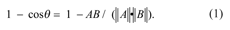
A cosine distance of 0 indicates that two vectors have identical directions, and a cosine distance of 2 indicates that two vectors have opposite directions. Two vectors are orthogonal if the cosine distance is equal to 1.

We chose simple, transparent methods for combining replicates, computing distances, and classifying profiles because our goal was to compare the core profiling methods rather than devise an optimal end-to-end analysis pipeline. In a real profiling application, other choices may be advantageous; for instance, the problem of classifying compounds into mechanisms is likely amenable to supervised classification approaches.

Profiling Methods

Means

The average is taken over all scaled features for each sample. Adams et al. ¹³ use this method but extend their profiles with means for different cell-cycle phases, some intensity proportions, and some standard deviations.

KS Statistic

The i-th element of the profile for a sample is the Kolmogorov-Smirnov (KS) statistic between the distribution of the i-th measurement of the cells in the sample with reference to mock-treated cells on the same microtiter plate. The KS statistic is calculated by taking the maximum distance between the empirical cumulative distribution functions (cdfs). Following Perlman et al., ¹⁴ we used a nonstandard “signed” KS statistic that indicates whether the maximum distance is positive or negative.

Perlman et al. ¹⁴ describe this method in the context of a more extensive methodology that compares compounds over a range of concentrations, trying different alignments of the compounds’ concentration ranges in order to produce a “titration-invariant similarity score.” This procedure is independent of the underlying core profiling method and could therefore be used with any of the five methods tested here. We did not use it because the cosine distance was a stable measure of profile similarity in our experiment, even across concentrations (data not shown).

Normal Vector to Support-Vector Machine Hyperplanes

Support-vector machines (SVMs) were trained to distinguish the cells in each sample from mock-treated cells on the same microtiter plate.

SVM recursive feature elimination (SVM-RFE) starts by training an SVM model to distinguish a treatment from DMSO. The prediction accuracy is estimated using cross-validation. The n measurements with the lowest weight are then removed, and a new model is trained using the remaining measurements. This continues iteratively until one feature remains. Finally, the SVM model with the best prediction accuracy is selected. The best feature selection accuracy is theoretically obtained by removing one feature at a time (SVM-RFE1); however, this is computationally expensive. Therefore, following Loo et al., ¹⁵ we used SVM-RFE2, which removes the 10% of the measurements with the lowest weight at each iteration. To eliminate more measurements, Loo et al. ¹⁵ eliminated measurements until the prediction accuracy fell below 0.9 × ((C_max – C_min) + C_min), where C_max is the maximum prediction accuracy and C_min the minimal prediction accuracy over the full range of a selected number of measurements.

Gaussian Mixture Modeling

To build Gaussian mixture (GM) profiles, 10% of the data were subsampled uniformly across all samples. This selection was mean-centered, after which the data were transformed using principal-component analysis (PCA), retaining enough principal components to explain 80% of the variance (~54 for our data set). Next, a GM model was fit to the data using the expectation-maximization (EM) algorithm. The algorithm was initialized with unit covariance and the centroid positions obtained using the k-means algorithm. The starting positions of the centroids in the k-means algorithm were initialized randomly, meaning the algorithm is nondeterministic. The Gaussians resulting from the EM algorithm were used as a model for the remaining 90% of the data. The rest of the data were centered using the mean of the data that was used to build GM models and projected into the same loading space. For each cell, the posterior probability of belonging to each of the Gaussians was computed. Profiles were constructed by averaging these posterior probabilities for each compound concentration. The number of values in a profile is thus equal to the number of Gaussians used to model the data. The best number of Gaussians was chosen empirically.

Factor Analysis

This method attempts to describe the covariance relationships between the image measurements x in terms of a few latent random variables y called factors. The factors are drawn from an isotropic Gaussian distribution. The observed image measurements x are modeled as an affine transformation Ay + µ of the factors and a measurement-specific noise term ν:

$$x=Ay+\mu +\nu .$$

The observed measurements are assumed to be conditionally independent given the factors; in other words, ν ~ N(0, Σ), where Σ = diag(σ₁, …, σ _d ). We estimate A, µ, and Σ by an EM algorithm ¹⁶ implemented in the MDP toolkit (http://mdp-toolkit.sourceforge.net/). Then, we can compute the profile of a sample as the maximum a posteriori estimate of y:

$$\text{E}\left[y|x_n\right]=A^{\text{T}}{\left(A{A}^{\text{T}}+\Sigma \right)}^{-\text{1}}\left(x_n-\mu \right)$$

where x _n is the vector of per-cell measurements in sample n averaged over the cells in the sample.

Available Data

To facilitate the development and evaluation of additional profiling methods, we provide our ground-truth annotations (Suppl. Table S2) and the measurements of each of the ~450,000 cells whose treatments are annotated. The data are supplied as comma-delimited files together with scripts for loading them into a MySQL database (Suppl. Data S2). The data schemas are described (Suppl. Text S1).

The images and metadata have been deposited with the Broad Bioimage Benchmark Collection (http://www.broadinstitute.org/bbbc/), ¹⁷ accession number BBBC021.

Software Implementations

The profiling methods are implemented as part of the open-source image data-analysis software CellProfiler Analyst (http://cellprofiler.org/). The implementations do not make assumptions that are particular to our experiment and can be readily applied to measurement data from the widely used image-analysis software CellProfiler^11,12 or data from other sources that can be imported into CellProfiler Analyst or otherwise converted to CellProfiler’s database schema. The implementations contain support for parallel processing on a cluster of computers. The profiling methods can be executed as scripts from the Unix command line or used in Python programs as a module (Suppl. Text S2).

Reproducibility

We provide complete source code to readily reproduce most figures, tables, and other results that involve computation (Suppl. Text S3; Suppl. Data S3). Supplemental Table S6 was constructed manually/interactively and is not reproducible.

Results

We implemented five proposed methods^{13–15,18,19} for constructing per-sample profiles from per-cell measurements in a common computational framework. We benchmarked the five methods on images we had previously collected of MCF-7 breast cancer cells treated for 24 h with a collection of 113 small molecules at eight concentrations (Suppl. Table S3). The cells were fixed; labeled for DNA, F-actin, and β-tubulin; and imaged by fluorescent microscopy. For this study, we measured 453 standard cytometric measurements (Suppl. Table S1) of each cell using CellProfiler^11,12 and applied each of the five profiling methods. To be able to evaluate the performance of the profiling methods, we limited our attention to a subset of the data (our “ground-truth” data set) for which we were confident that the primary MOA of compounds was achieved at the concentration tested during the course of the experiment. (The term mechanism of action is used rather loosely here and refers to a sharing of similar phenotypic outcomes among different compound treatments, rather than referring strictly to modulation of a particular target or target class.) The mechanistic classes were selected so as to represent a wide cross section of cellular morphological phenotypes. The differences between phenotypes were in some cases very subtle: We were able to identify only 6 of the 12 mechanisms visually; the remainder were defined based on the literature. This carefully collected ground-truth data set consisted of 38 compounds at active concentrations. Some compounds were active at only one concentration and some at up to seven concentrations, for a total of 103 treatments (active compound concentrations) spanning 12 mechanistic classes (Suppl. Table S2; Suppl. Fig. S1). The mock treatment DMSO was included as a negative control. Using the cosine distance as a measure of profile dissimilarity, we classified the 103 treatments into MOAs by assigning to each profile the MOA of the most similar profile ( Fig. 1 , top). When classifying a treatment, all concentrations of the same compound were held out from the training set in order to prevent overtraining. The samples were prepared and imaged in 10 batches, but classes and replicates were distributed across batches and plates, respectively, so as to avoid biasing the classification (Suppl. Text S4). ²⁰ Using this experimental data set, we tested five profiling methods ( Fig. 1A – E ), as detailed below.

Figure 1.

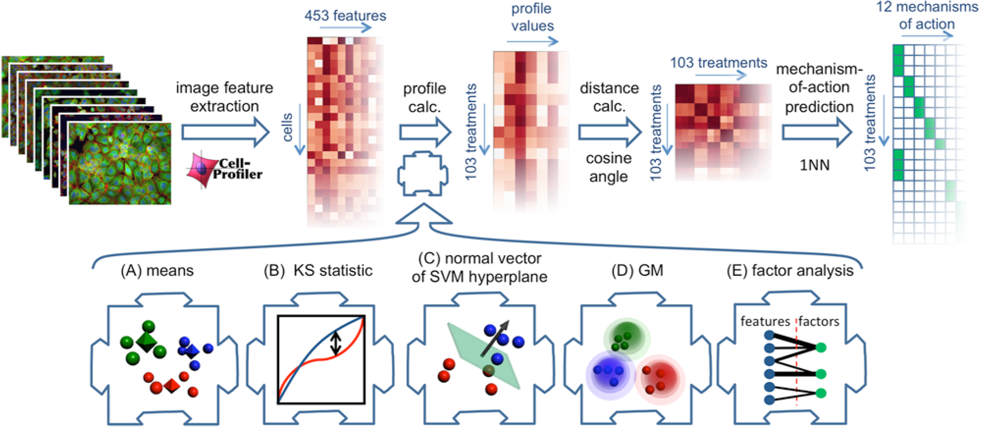
Overview of approach. (Top) Experimental design. Cultured cells in microtiter plates were compound treated, labeled, fixed, and imaged. The image analysis software CellProfiler measured 453 properties of each cell. One of the profiling methods under investigation condensed these measurements into a profile (vector of numbers) that describes each sample. A sample with unknown mechanism of action (MOA) was predicted to have the same MOA as the sample whose profile is most similar to that of the unknown sample, using the cosine of the angle between the profiles as measure of similarity. (Bottom) Illustrations of the five profiling methods tested. (A) Means of raw per-cell features. (B) Kolmogorov-Smirnov (KS) statistic relative to negative control. (C) Normal vector of decision plane of linear support-vector machine (SVM) versus negative control. (D) Proportion of cells in each component of a Gaussian mixture (GM). (E) Latent feature extraction using factor analysis.

Means

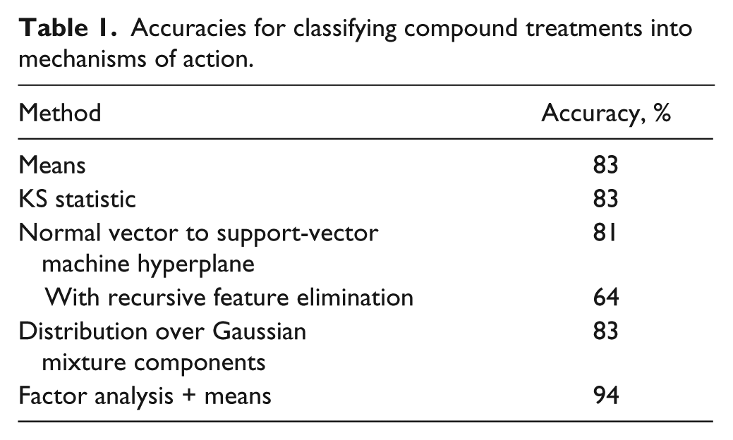
We first constructed profiles in the simplest way we could envision: average each measurement over the cells in the sample ( Fig. 1A ). A profile thus consists of a single value for each of the 453 features. This was the main approach used by Tanaka et al. ²¹ to discover an inhibitor of carbonyl reductase 1, although their profiles also included some statistics other than the mean. ¹³ With this profiling method, 83% of the compound-concentration profiles could be classified correctly ( Table 1 ). The cosine distance remained effective despite the high dimensionality of the measurements, so there is no significant compression of distances, a common problem in high-dimensional data analysis in which the distance to the nearest point approaches the distance to the farthest point (Suppl. Fig S2). This indicates that most of the measurements contribute information about MOA and are not simply redundant measurements that add noise. ²²

Table 1.

Accuracies for classifying compound treatments into mechanisms of action.

Method	Accuracy, %
Means	83
KS statistic	83
Normal vector to support-vector machine hyperplane	81
With recursive feature elimination	64
Distribution over Gaussian mixture components	83
Factor analysis + means	94

That small-molecule effects could be characterized so well by the shift in means was unexpected because many treatments induce a heterogeneous phenotypic response across the cell population in each sample. For instance, treatment with microtubule destabilizers produced a mixture of ~44% mitotic cells, ~27% cells with fragmented nuclei, ~16% cells with diffuse and faint tubulin staining, and ~12% cells with an appearance similar to mock-treated cells. Even though the “means” method made no attempt to model the subpopulations of cells, it was mostly able to distinguish microtubule destabilizers from microtubule stabilizers, which also block in M-phase and therefore also caused a high proportion of mitotic cells (Suppl. Table S4). There was room for improvement, however; in particular, many microtubule stabilizers and actin disruptors were misclassified as other MOAs. DNA damage agents and DNA replication inhibitors were consistently confused.

Although the image features that are most influential in distinguishing each mechanism of action from the rest (Suppl. Table S5) are largely expected (e.g., the texture of actin staining in the cytoplasm is important for distinguishing actin disruptors), it is notable that the profiles generally obtain their discriminatory power from a combination of image features.

Some other population statistics (medians, modes, and means combined with standard deviations) gave similar results. Medians combined with median absolute deviations achieved higher accuracy (88%), mainly by being better able to distinguish DNA damage agents and DNA replication inhibitors (Suppl. Fig. S3).

KS Statistic

Perlman et al. ¹⁴ used the KS statistic as part of their titration-invariant similarity score profiling method. The KS statistic is calculated separately for each treatment and measurement. It is the maximal difference between the cumulative distribution function (cdf) of the measurements of the treated cells and the corresponding cdf of mock-treated cells ( Fig. 1B ). This method is more computationally expensive than simply computing the mean but can be more sensitive: For example, a hypothetical treatment that causes some of the cells to shrink and the rest to grow could leave the mean cell size unchanged but would increase the KS statistic.

The method based on the KS statistic reaches a prediction accuracy of 83% ( Table 1 ). As with the means method, DNA damage agents and DNA replication inhibitors were confused (Suppl. Fig. S4B). Many DNA damage agents were additionally misclassified as Aurora kinase inhibitors, and there was some confusion between microtubule destabilizers and Eg5 kinesin inhibitors.

Normal Vectors to SVM Hyperplanes

Loo et al. ¹⁵ describe a multivariate method that trains a linear SVM ²³ to distinguish compound-treated cells from mock-treated cells. The SVM constructs the maximal-margin hyperplane that separates the compound-treated and mock-treated cells in the feature space. The normal vector of this hyperplane is adopted as a profile of the sample ( Fig. 1C ). The method classified 81% of the treatments correctly ( Table 1 ).

The methodology of Loo et al. ¹⁵ additionally uses SVM-RFE to remove redundant and noninformative measurements from profiles and replace them with zeros in order to increase the sensitivity of analysis and make profiles more interpretable. This feature elimination is done independently for each treatment. Adding this step reduced the classification accuracy to 64% ( Table 1 ). Inspecting the lists of features chosen gives a clue to why: The SVM is being trained to distinguish a compound from DMSO, so the features most useful for this purpose are selected. These features are not generally the same features that are useful for distinguishing compounds with different MOA. Indeed, features preferentially retained by the feature-elimination step are often correlated with reduced cell count, as almost every active compound has some cytotoxic effects: Three of the five most frequently selected features are clearly influenced by cell count, having to do with number of neighbors and number of cells touching (Suppl. Table S6). This behavior is not a flaw in SVM-RFE: It simply magnifies the tendency of the normal-vector method to emphasize the features that most clearly separate the treated cells from mock-treated cells.

Distribution over GM Components

To better characterize heterogeneous cell populations, Slack et al. ¹⁸ proposed modeling the data as a mixture of a small number of Gaussian distributions and profiling each sample by the mean probabilities of its cells belonging to each of the Gaussians. This GM method assumes that compound treatment causes cells to shift between a limited number of general states. It is indeed generally true that cellular phenotypes induced by perturbations can usually be found, albeit at low levels, in wild-type cell populations. ⁵ GM models have been used in other phenotype-detection applications as well. ²⁴

We fitted different mixtures of Gaussians to a subsample of ~45,000 cells (10% of the cells), with the number of components ranging from 2 to 30. A nondeterministic EM algorithm was used to fit Gaussians to the data; therefore, the model construction and cross-validation was performed 20 times to assess model variability. Twenty-five Gaussians resulted in a prediction accuracy of ~83% ( Table 1 ) but with large variation depending on the initial conditions (Suppl. Fig. S5). Increasing the number of Gaussians beyond 25 does not improve the accuracy (Suppl. Fig. S5). Some classification mistakes occurred in only some models, whereas others were consistent across models (Suppl. Fig. S4E).

The GM method performs equally well whether created from control cells or treated cells (Fig. S6), so the mixture components may be mainly modeling cellular phenotypes that are widely represented rather than phenotypes induced by only particular treatments.

Factor Analysis

Although we measured 453 morphological features of each cell, it is the underlying biological effects that are of interest. Young et al. ¹⁹ used factor analysis to discover such underlying effects under the assumption that an underlying process (factor) affects several measurements and that variations restricted to a single measurement are noise.

We trained a factor model on a random subsample of ~45,000 control cells (15% of the control cells in the experiment). We computed the maximum a posteriori estimate of the factors given each cell and averaged these values over all cells treated with the same compound and concentration to obtain a profile of the treatment. Varying the number of factors, we found that the performance was similar to the other methods when using ~25 factors but that performance increased gradually with the number of factors, reaching a plateau at ~50 factors ( Fig. 2 ). Although the procedure is nondeterministic, the accuracy generally does not change more than 3 percentage points in either direction with a given number of factors. With 50 factors, the prediction accuracy was 94%, which is substantially better than any of the other methods that were tested ( Table 1 ). There was still some confusion between DNA damage agents and DNA replication inhibitors ( Fig. 3 ).

Figure 2.

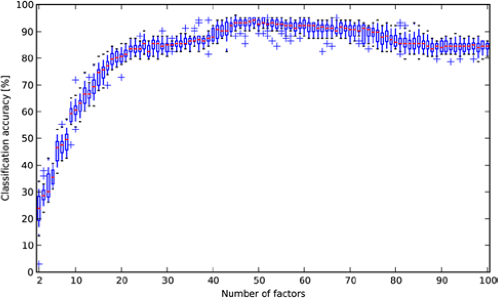
Distributions of classification accuracies for 20 runs of the factor analysis method for each possible choice of the number of factors from 2 to 100. The performance was similar to the other methods when using ~25 factors, but the accuracy increased gradually with the number of factors, reaching a plateau at ~50 factors.

Figure 3.

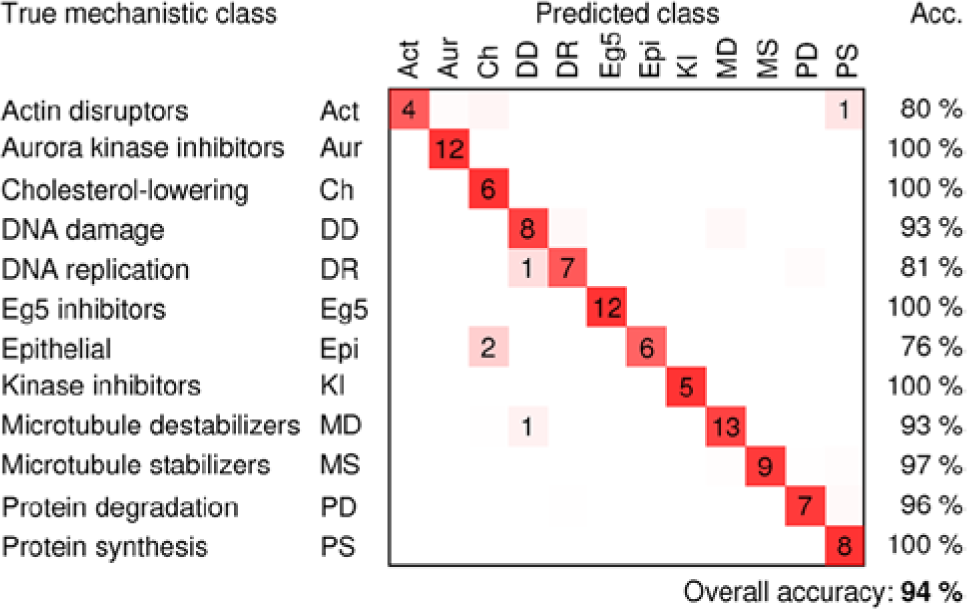
Confusion matrix for the factor-analysis method, showing the number of compound concentrations that were classified correctly (on the diagonals) and incorrectly (off the diagonals), the classification accuracies for each mechanism of action (right columns), and overall classification accuracy (number of correctly classified compound concentrations divided by the total number of compound concentrations). Average outcomes over 20 models are shown; dimly colored squares without numbers indicate classification outcomes that occurred fewer than 0.5 times on average.

The improvement in accuracy was not simply due to the method’s implicit dimensionality reduction: Reducing the dimensionality to 50 by PCA did not lead to an improvement over the means method, and selecting the feature most heavily loaded on each of the 50 factors decreased the accuracy to 63% (Suppl. Table S7).

The factor-analysis method can be viewed as the means method with a preprocessing step that transforms the measurements of each cell into the latent factor space. Although factor analysis greatly improves the means method, it does not improve the KS statistic method as much. Using it as a preprocessing step before any of the other profiling methods is not helpful (Suppl. Fig. S7).

Most of the factors cannot be readily interpreted by their feature loadings (Suppl. Table S8). This is an Occam dilemma ²⁵ : When the number of factors is high enough to yield good predictive accuracy, the factors are difficult to interpret because they combine numerous features in order to pick up on subtle phenotypic differences. Although we cannot use direct interpretation to verify that the factors are biologically relevant, careful cross-validation and experimental design can guard against bias by batch effects and other artifacts ²⁰ (Suppl. Text S4).

The factor model performs equally well whether created from control cells or treated cells (Suppl. Fig. S9). Because the wild-type variation is sufficient to elucidate the relationships between image features and latent factors, the factors may be capturing stable, fundamental modes of variation for the cell line (viewed through a particular assay and feature set) and not the extreme changes induced by particular treatments.

Discussion

We compared five methods^{13–15,18,19} for generating per-sample profiles from image-based cell data in the context of classifying small molecules into 12 MOAs based on cellular morphology. All methods had previously been demonstrated in distinct experiments, mostly proof-of-principle studies, with some yielding biological discovery. However, these methods had never before been directly compared on a common data set. Each method was previously proposed as part of a larger methodology, sometimes including strategies for particular contexts, such as making use of information from multiple cell lines or multiple concentrations. These strategies can be applied independently of the core profiling method; here, we compared only the computational cores of the profiling methods. We did not evaluate the underlying statistical methods (KS, SVM, GM, factor analysis), which have solid theoretical foundations and an excellent record of solving analysis problems of many kinds.

On our data set, the simplest method, which profiles compounds by the population means of the measurements of the treated cells, performed better than expected, achieving 83% accuracy in predicting MOA. Because many of the measurements are non-Gaussian, we expected nonparametric KS statistics to be superior, but that was not the case. Describing a compound by the decision boundary of a linear SVM trained to distinguish compound-treated cells from mock-treated cells did not offer improvement either (83%), and adding a feature-reduction step reduced performance (64%). A GM method that tries to model subpopulations of cells with a mixture model might be expected to have an advantage in experiments in which the perturbations lead to shifts between a small number of discernible cell states (e.g., cell-cycle states), but we did not observe this: Although the treated samples were heterogeneous with respect to cellular phenotype, and some phenotypes were not specific to any mechanistic class, the GM model performed no better than other methods (83%). The profiles that best represented the phenotypes were obtained using factor analysis (94% accuracy in predicting MOA). This method’s potential limitation of excluding important nonredundant image-based features as noise has been demonstrated in a screening context in which only 29 measurements were made of each cell, ²⁶ but with our higher-dimensional features, the method proved effective at extracting the underlying sources of variation.

Because all of the profiling methods we tested operate on measurements at the resolution of single cells, there was the potential that some of them might detect effects that are present in only a small subpopulation of the cells in the sample. However, only the GM method makes explicit attempts to model cell subpopulations across samples. It was therefore surprising that even the means method was sufficient to characterize treatments producing heterogeneous phenotypic response. Because compound treatments typically affect most cells in a sample (although frequently in different ways), our experimental results are insufficient to predict the methods’ relative performance in RNAi screens in which the interference is effective in only a small percentage of the cells. It is possible that the KS statistic may work better than the mean in such experiments or that the GM method may be able to detect a globally popular phenotype even though it occurs at a low proportion in a particular sample. It is also possible that new profiling methods will be required to fully realize the potential of using single-cell measurements to profile samples that are distinguished only by small, subtle subpopulations of cells or to be robust to off-target effects.

The assay and compound collection chosen for this study are typical of a profiling experiment: Morphology assays are attractive for profiling because they can capture a wide variety of subtle cellular responses without focusing on particular pathways. However, there may be particular MOAs that are not displayed within the assay parameters described in this study. One important parameter is time following compound exposure. In this study, we chose 24 h following compound treatment of cells as this produced an optimal mitotic arrest phenotype in the MCF-7 cell line studied. For other cell lines or other compound classes, there may be added value gained from increasing the biological space of profiling studies by combining features quantified from multiple assays and applying the profiling methods across multiple time points following compound treatment. The choice of assay and optimal time point for profiling will likely depend on the scientific questions being asked. The chemical compounds we tested are commonly studied bioactive compounds. Therefore, the present study is valuable in providing a comparative analysis of methods in the context of one particular (but representative) profiling experiment. Creating and annotating a ground-truth set of compounds with known MOA is not trivial; we hope this work provides a template for future creation of ground-truth data sets.

With the emergence of image-based high-content screening across more complex and diverse assay formats incorporating co-cultures, stem cells, and model organisms, future studies may demonstrate that particular profiling methods perform better on specific assays, cell types, or even focused compound or siRNA libraries. Thus, we foresee additional value in providing an analysis framework and a ground-truth data set to facilitate further comparisons in the field using alternate data sets or methods. We have implemented all five methods and offer the source code (Suppl. Text S2), along with our entire set of cellular measurements for our ground-truth data set (Suppl. Data S2) so that they can aid in the future application, development, and comparison of image-based phenotypic profiling approaches.