
Abstract
Imaging-based high-content screens often rely on single cell-based evaluation of phenotypes in large data sets of microscopic images. Traditionally, these screens are analyzed by extracting a few image-related parameters and use their ratios (linear single or multiparametric separation) to classify the cells into various phenotypic classes. In this study, the authors show how machine learning–based classification of individual cells outperforms those classical ratio-based techniques. Using fluorescent intensity and morphological and texture features, they evaluated how the performance of data analysis increases with increasing feature numbers. Their findings are based on a case study involving an siRNA screen monitoring nucleoplasmic and nucleolar accumulation of a fluorescently tagged reporter protein. For the analysis, they developed a complete analysis workflow incorporating image segmentation, feature extraction, cell classification, hit detection, and visualization of the results. For the classification task, the authors have established a new graphical framework, the Advanced Cell Classifier, which provides a very accurate high-content screen analysis with minimal user interaction, offering access to a variety of advanced machine learning methods.
Introduction
H
Multiparametric and nonlinear—follow the fashion
Occam’s razor principle states that “entities must not be multiplied beyond necessity” (entia non sunt multiplicanda praeter necessitatem) and the conclusion thereof, that the simplest solution is usually the correct one. In many HCS experiments, the use of simple parameters and thresholding can be very effective and robust, 1 but this may not be sufficient, depending on the actual parameter distribution.
To illustrate the problem, we give a few synthetic classification examples, moving from simple to more complex situations. Figure 1A shows an example where two data sets represented by two features can be completely separated with a straight line (i.e., ratio between the features). This simple ratio-based solution has many advantages, such as easy interpretation, computational cost-efficiency, and robustness. A more difficult case is depicted in Figure 1B . The two data sets cannot be separated anymore by a simple straight line without significant errors. Nonlinear separation techniques offer a solution for the problem. Figure 1C shows an extreme situation, which still can be handled by highly nonlinear classification, but this may result in the loss of generality. In this case, one should probably reconsider the feature set and, if possible, change to or introduce new features as shown in Figure 1D . When increasing the number of features, one should still keep in mind the “curse of dimensionality”: The data volume increases exponentially with the additional dimensions, and hence one needs exponentially more training examples. For further reading, see Hastie et al. 2 and Duda et al. 3
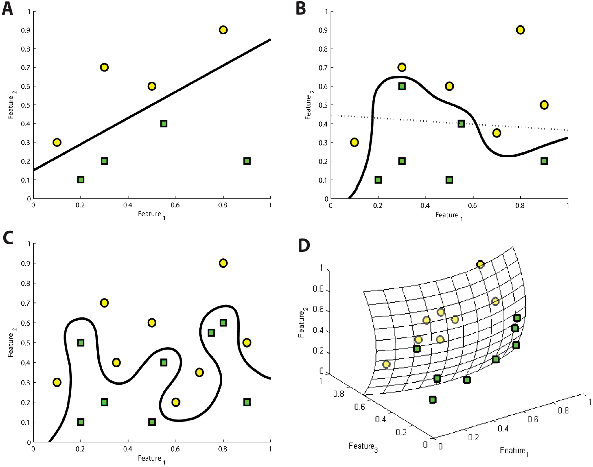
Linear versus nonlinear separation. (
In this article, we have investigated (using a real biological case study) whether and to which extent can the increase of a number of features increase the accuracy of the analysis and whether and to which extent can complex classification methods outperform simple ones. The performance of the methods was determined by measuring cross-validation accuracies and analyzing the receiver operating characteristic (ROC) curves.
Recently, some have proposed using machine learning approaches to analyze single-cell-based high-content screens, and as a result, various software packages have been published.4–6 Our solution, the Advanced Cell Classifier (ACC), presented in this article, offers two additional features: First, ACC is not limited to a specific classifier (usually the support vector machine), 3 and second, our approach can detect even very small phenotype changes, allowing one to identify not only the main but also subphenotypes. Here we concentrate on only the artificial neural network (ANN) classifiers as they are one of the best known, but others can also be used and are implemented in the package.
Assay quality is one of the most important criteria when evaluating a screen. One of the most frequently used parameters to characterize the quality of a screen is the Z factor. 7 For “traditional” (single-parameter readout) screens, this works nicely. However, as high-content screens deliver a large number of parameters (e.g., the results of the image processing), interpretation of a Z factor is not trivial. It is often sufficient to select one of the parameters because in many screens, the most significant one can be easily identified, and calculate the Z factor for this selection. Nevertheless, this approach can be problematic for many image-based screens as imaging data can be relatively noisy, and it does not make use of the multitude of the available parameters, the main advantage of an HCS approach. Recently, a multiparametric interpretation of the Z factor was described 8 but using only linear separation between entities, which is not the case for most of the novel machine learning approaches. Here, we calculate the Z factor for nonlinear classification results and show that by using machine learning methods, we were able to considerably improve the quality of a specific image-based siRNA screen.
In the following section, we first introduce the specific biological problem and screening approach used for this case study. Afterwards, we discuss the data-processing pipeline used to evaluate the screen. This will be followed by the comparison of the various classification approaches.
Materials and Methods
The biological question/screening approach
Ribosomes are universally conserved macromolecular complexes used for protein synthesis. They consist of two ribosomal subunits, termed small and large, which are composed of ribosomal RNA (rRNA) and ribosomal proteins. In eukaryotes, the generation of these subunits is a complex, multistep process, which takes place in different cellular compartments. Early ribosomal subunit precursors are assembled in the nucleolus, the place of rRNA transcription. Subsequently, these precursors pass through the nucleoplasm and are exported to the cytoplasm, where final maturation steps occur and both subunits join to function in protein synthesis. 9
The target of our investigation was the biogenesis of the small ribosomal subunit in human cells (40S subunit). 10 Toward this, an assay for visual detection of nuclear maturation defects of the 40S subunit was developed. 11 In short, a HeLa cell line bearing a fluorescently tagged ribosomal protein of the 40S subunit (Rps2-YFP), which is expressed only upon induction (by TET activation), was used to selectively visualize newly synthesized 40S subunits. Within the period of induction (14 h), the majority of the newly made 40S subunits reach the cytoplasm—that is, a strong Rps2-YFP signal is detected in the cytoplasm (class a in Fig. 2B ). However, if nucleolar or nucleoplasmic 40S maturation steps are impaired, the Rps2-YFP signal accumulates in the respective nuclear subdomain, whereas the cytoplasmic signal is diminished (classes e and f). Besides these strong nuclear accumulation phenotypes, more subtle phenotypic variations also can be distinguished (classes b–d).
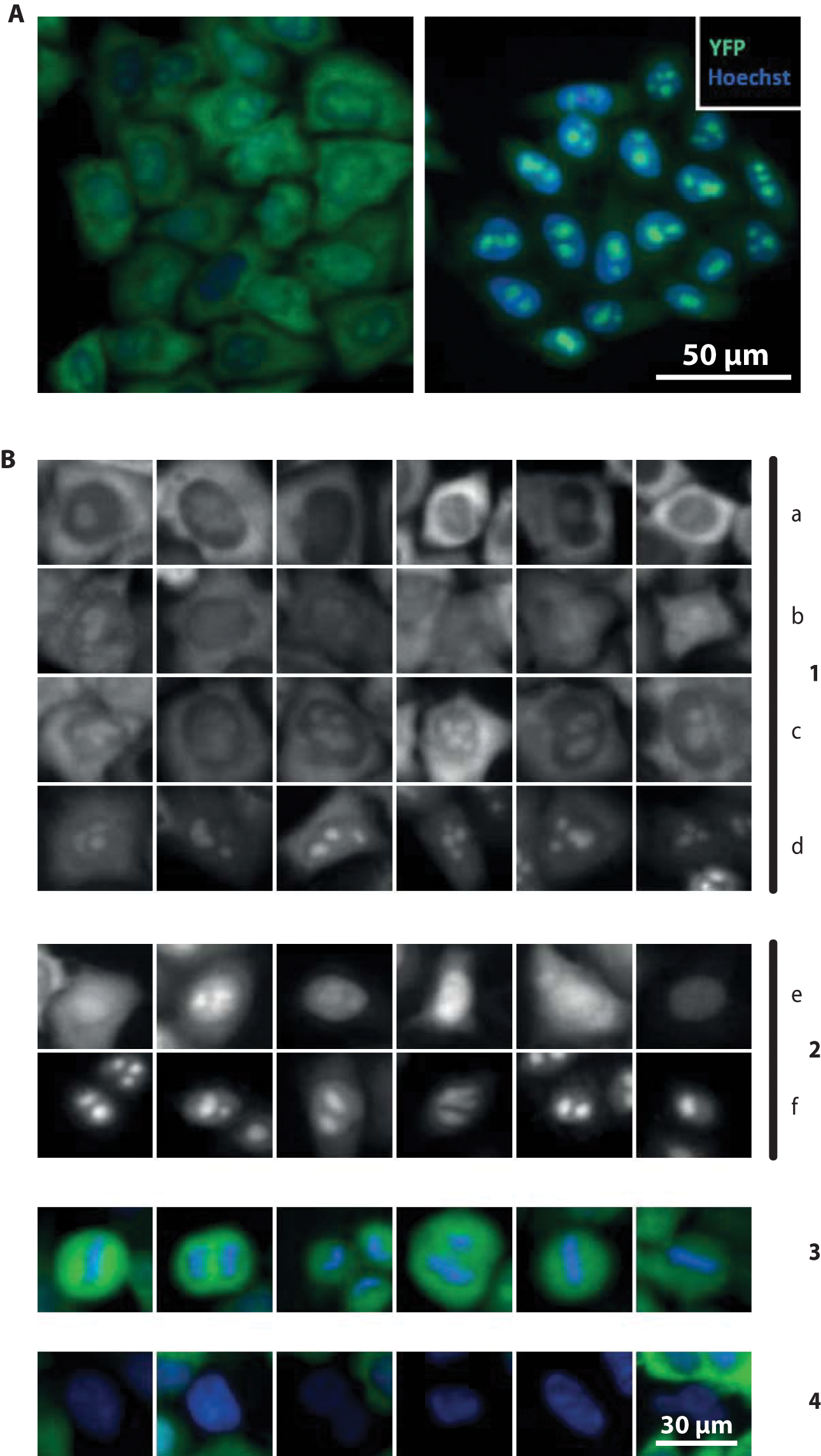
(
We used this assay to detect nuclear 40S maturation defects upon depletion of a protein by RNAi. This allowed us to identify proteins functioning in 40S biogenesis in human cells and, according to the classification, assign their requirement to nucleolar or nucleoplasmic maturation events.
Data-processing pipeline
Our data-processing pipeline consists of three major parts. The first one, dealing with image processing and feature extraction, is based on CellProfiler. 12 The second step involves classification of the cells into predefined clusters using machine learning algorithms or ratio-based thresholding using our ACC. The third part includes annotation and quantitative evaluation of the data.
Figure 3 summarizes our data analysis pipeline. We use CellProfiler to identify cells and extract their features. First, we detect the cell nucleus on the blue channel (Hoechst staining of chromatin) with an adaptive threshold. We exclude objects smaller than 6.5 µm and bigger than 48 µm in diameter because according to our experience, all cell nuclei (in all cell cycle stages) of the used HeLa cell line should be within these dimensions. Hence, this step eliminates objects originating most likely from noise or dirt. We also discard objects touching the image boundaries. Second, we create a mask for the cytoplasm. The most precise way would be to detect the entire cytoplasm and use it as a mask, but in our positive controls, the marker is localized exclusively on the nucleus. Therefore, we cannot directly detect the cytoplasm. Introducing an additional fluorescent dye/channel would have been an option, but it would have seriously complicated the experimental procedures. To solve this problem, we have therefore chosen the following workaround, which has been proven to be successful in many previous studies: We defined a 3.9-µm wide ring around the nucleus and used this as a cytoplasm mask. This particular value is based on our experience and is true for the used HeLa cell line. Visual inspection confirmed that we adequately captured a cytoplasmic signal with this dimension. As a next step, we measured the mean fluorescence intensity and its standard deviation in the blue and green channels using the nucleus and cytoplasm masks, respectively. We also calculated morphological descriptors of the nucleus (e.g., area) and extracted texture information from both channels. Using this image segmentation process, we have extracted 26 different intensity, shape, and homogeneity features and used those to perform the classification. As a last step, we convert and save our images for visualization purposes: a compressed color image combining the original channels, an image overlaying the object outlines, a montage image combining the nine images taken in each wells, and two smaller icon images for browsing purposes.
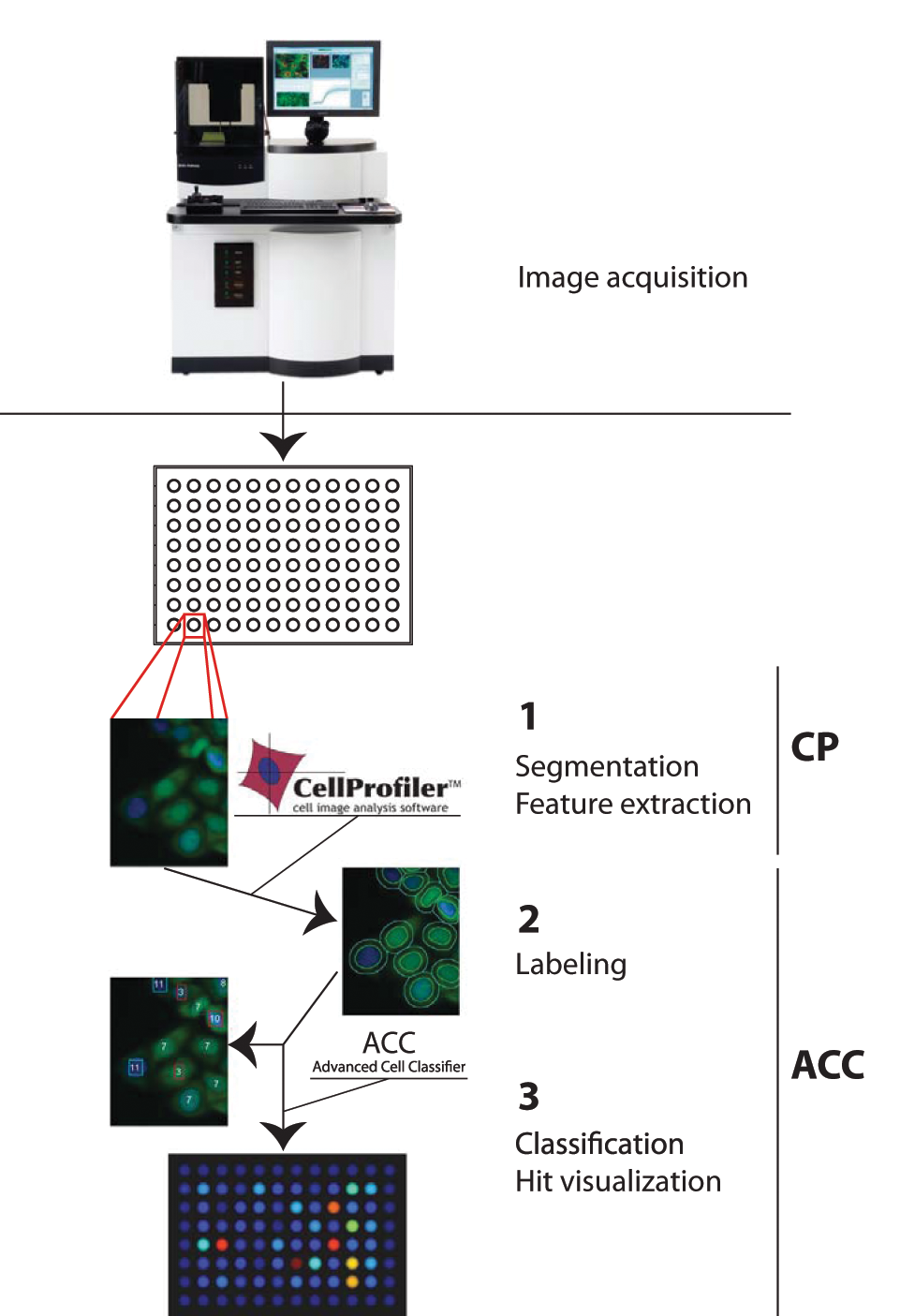
The three steps of the data-processing pipeline. Raw microscopic data are segmented and single-cell properties are extracted using CellProfiler. Advanced Cell Classifier is used to label phenotypes, train classifiers, perform supervised classification on the whole data set, calculate statistics, visualize results, and create reports.
For the classification task, because of the lack of suitable software solutions, we have developed custom software called the Advanced Cell Classifier. The system provides the following main features: graphical user interface to create training database for classification, immediate image classification, plate browser, report generation, and numerous classification algorithms. The code is written in MATLAB, and therefore it is platform independent, and further requirements can be easily implemented. We integrated the Weka framework, 13 which provides a huge variety of classification algorithms. To allow a more sophisticated analysis, our system allows biologists not only to define their main phenotypes but also to create subphenotypes. In our screens, we usually define four to six main phenotypes and two to four subphenotypes. According to our experience, we can reach 85% to 95% accuracy on the main types and 65% to 75% on the subphenotypes using ANN. The accuracy is calculated with the Weka Experimenter software tool using 10 times randomized 10-fold cross-validation. The ACC system also provides numerous quantitative data evaluation opportunities, such as ratio-based, classification-based, and cumulative statistics, where the user can define types/subtypes to exclude and/or merge together. To present the results, ACC offers a report generator and a high-throughput screening browser (http://www.cellclassifier.org).
Results
Classification
One of the major aims of this study is to compare simple human decision-based linear classification (termed ruler based) and a simple Bayesian classification method 14 to ANN and investigate whether and how additional features can improve the classification accuracy. For the comparison, we prepared two training sets, both of them containing 500 cells. The first set distinguishes between five major phenotype classes, * whereas the second contains nine different classes, from which four and two are the subclasses of the negative and positive control phenotypes, respectively, as described earlier and shown in Figure 2B .
The realization of the ruler-based method was performed such that a printed paper was shown to the human observer and linear separation lines were drawn. It needs to be mentioned that applying a ruler-based method for nine classes turned out being an unrealistic aim, and therefore this analysis was performed only for the five major classes. The naive Bayesian classification method was chosen to test the behavior of a simple classification method and compare its performance on the same problem to a more complex method such as ANN.
Artificial neural networks
An ANN is a computational model based on biological neural networks. 3 It is a collection of input units and processing units, called artificial neurons, that are interconnected on several layers. In general, an ANN is an adaptive system that changes its structure during the learning phase. In signal processing, ANNs are used to model complex relationships between input and output data. Neural networks are different from computers in the sense that they “learn” to solve problems. The network compares the results of its prediction with the desired output, which is in our case provided as labeled cells. The discrepancies between the desired output and that of network error are then minimized up to a tolerance level.
ANN versus human observer
First, we compared the classification ability of the ANN model, the naive Bayes classifier, and the linear separation based on the human observer’s decision. As visualization and human interpretation of more than two features is rather complex, we decided to choose the two most important ones by determining the impact of all 26 individual features using Weka’s Info-Gain † method to evaluate them. Table 1 shows the ranking and impact of the 10 most important attributes.
Top 10 Features Ranked by Info-Gain
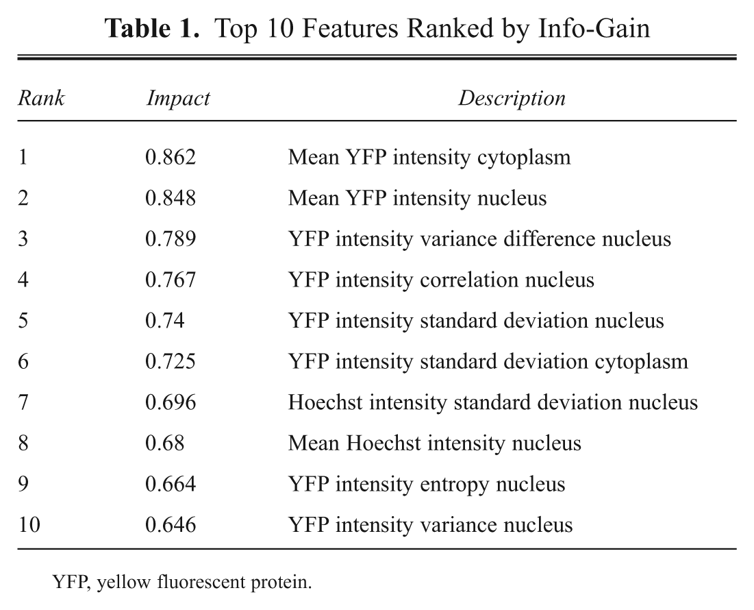
YFP, yellow fluorescent protein.
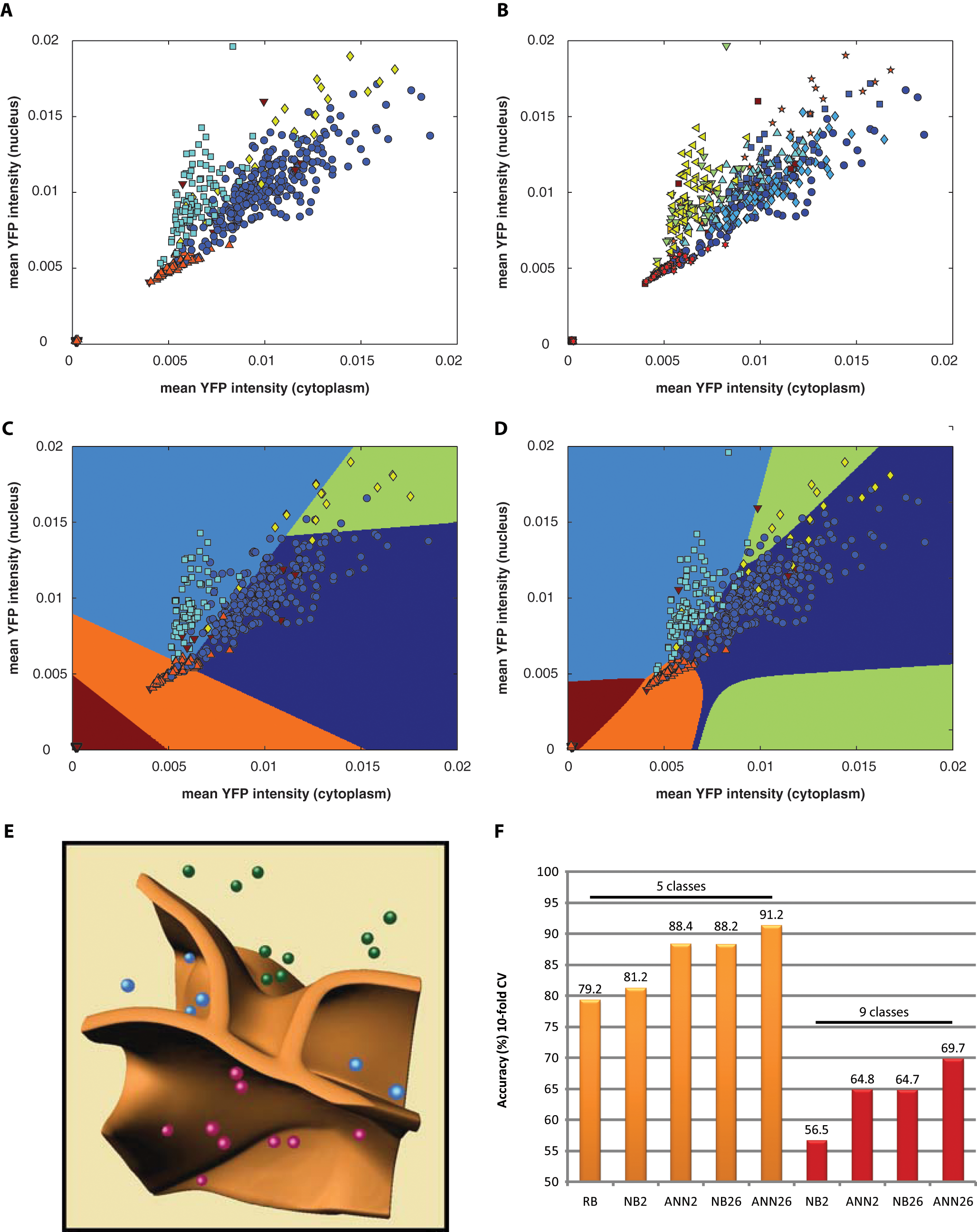
As expected, the two most reliable features were the mean of the YFP signal intensity on the cytoplasm and on the nucleus. We have distinguished between five main phenotypes, as described earlier. Figure 4A , B shows the labeled objects (five or nine phenotypes, respectively), and each individual class is labeled with a different color and marker. The biologist used a simple ruler-based method, trying to best separate classes with straight lines. An example is shown in Figure 4C . To measure the accuracy of the manual method, we used threefold cross-validation. In practice, this means that we split the data set into 66%–33% parts, did ruler separations on the first while evaluating the second part, and repeated this procedure three times. The achieved accuracy was 79.2%. Comparison to the naive Bayes and ANN ‡ methods using the same input data set is presented in Figure 4F . For the precise validation of the latter two methods, we used the Weka Experimenter framework and present the mean values of a 10-time repeated randomized 10-fold cross-validation. The standard deviation of these cross-validation measurements was in the range of 0.5%.
(
Figure 4D shows the regions separated by the ANN. It is worth noting that the decision boundaries are nonlinear and the accuracy is 88.4% (as shown in Fig. 4F ), and hence it clearly outperforms the linear classification (79.2%) and the naive Bayes methods (81.2%).
More features and more classes
To test the effect of additional features on the classification accuracy, we used 26 features instead of the two most important ones (as used in the previous step). Importantly, through this, the accuracy could be further increased both for the naive Bayes approach (from 81.2% to 88.2%) and for the ANN method (from 88.4% to 91.2%).
In our last experiment, we used the same labeled data set as previously, but we distinguished nine cellular phenotypes instead of the previously used five. Again, we tested the classification performance of the ANN and naive Bayes models using first only 2 and afterwards all 26 features. The results are presented in Figure 4F . In Figure 4E , we present the decision boundaries of the ANN classifier using the three most relevant features ( Table 1 ). Different colors of spots present different phenotypes. The graph nicely demonstrates the nonlinear nature of the method.
Z factor analysis
The above-presented increase of classification accuracy in the case of ANN may appear not so crucial for the overall performance of the screen. Therefore, we wanted to test whether the quality of the screen/assay (usually characterized by the Z factor) is affected if we use ruler separation, the naive Bayesian, or the ANN framework. For the calculation, we have used the positive and negative controls of the experiment described earlier. To do this, the hit rates of the controls were calculated as follows: R H = |C H | / (|C H | + |C N |), where |C H | and |C N | are the number of cells classified as hits and nonhits, respectively. Thus, R H is the ratio of hit-type cells over all biologically relevant cells. We determine R H value for all positive and negative control wells, and using the well-known Z factor, 7 we determine the separation ability of the analyzed methods with 2 features as well as for the ANN and the naive Bayes with 26 feature classifications. The results of the analyses are summarized in Table 2 .
Z Factor of Different Evaluation Methods
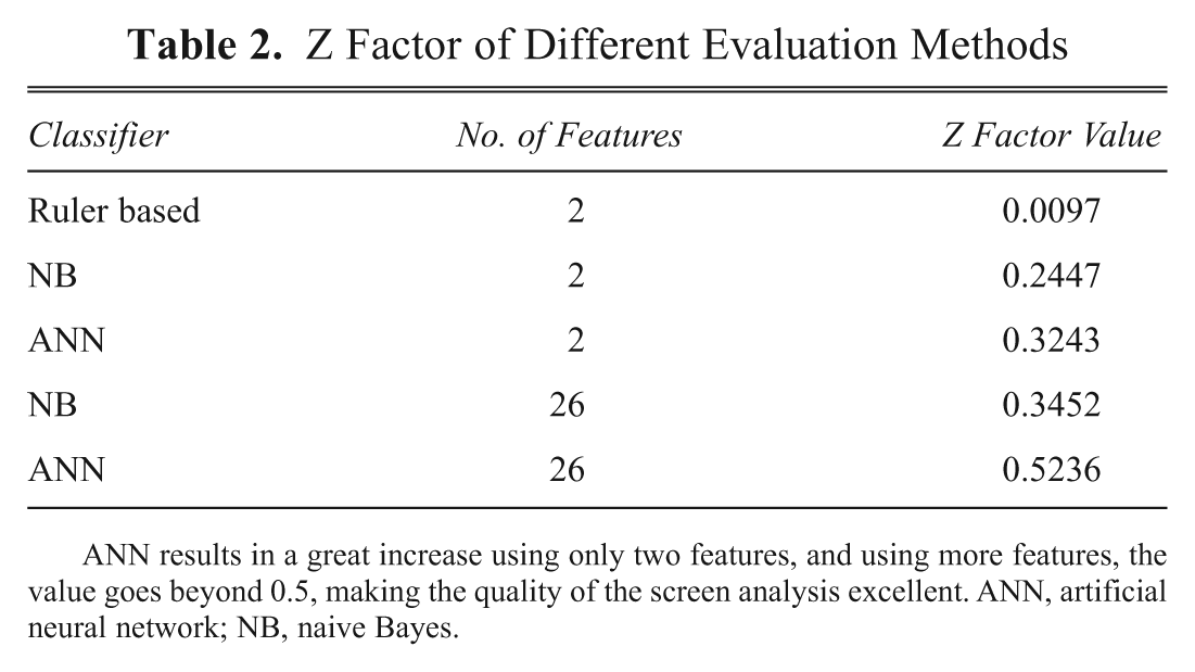
ANN results in a great increase using only two features, and using more features, the value goes beyond 0.5, making the quality of the screen analysis excellent. ANN, artificial neural network; NB, naive Bayes.
The Z factor values in Table 2 show the real strength of the ANN approach. Using the ruler-based method results in a relatively poor assay where the controls are almost overlapping, and this may result in a hit detection problem. Using the naive Bayes and ANN only with 2 features makes the readout already more stable, and with all 26 features, the Z factor further increases and is over 0.5 for the ANN, indicating a high-quality assay.
ROC analysis
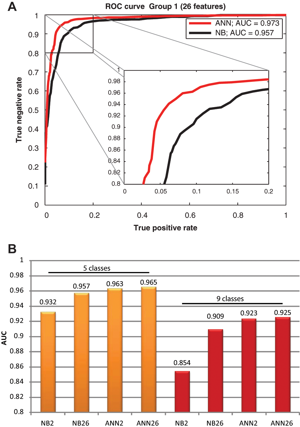
Classification error rate measurements give precise information about correctly and incorrectly classified instances, but they cannot distinguish between true-positive and false-positive instances, which for certain applications (e.g., disease prediction) can be very important. To further characterize classification accuracy, we analyzed the ROC curves and measured the area under the ROC curves (AUC).15,16 An ROC curve is a two-dimensional plot containing true-positive rates on the x-axis and false-positive rates on the y-axis for one particular class. It represents the trade-off between benefits (true positives) and costs (false positives). In practice, the optimal ROC curve connects the (0, 0), (0, 1), and (1, 1) points, and a random classifier would be a diagonal line between (0, 0) and (1, 1). In Figure 5 , we present the ROC and AUC analysis of the naive Bayes and ANN classifiers. Figure 5A shows an example ROC curve. The curve was determined using the threshold averaging technique described in Fawcett 15 with 10 ROC measurements. We can observe that ANN majorates the naive Bayes classifier in this particular case. For more general analysis in Figure 5B , we show the average of the AUC values using the cross-validation method described earlier. The values for ANN are higher in every case than for the naive Bayes, but in certain cases, this difference is not as pronounced as for the cross-validation accuracy. Discrete classifiers, such as the proposed ruler-based method, resulted only in a single point in the ROC space, and therefore measurements were not taken.
Receiver operating characteristic (ROC) curve and area under an ROC curve (AUC) evaluation. (
Discussion
In our studies, we compared the ruler-based separation to the naive Bayes and ANN methods. The most important advantage of the linear, human decision-driven method is that it is easy to interpret and visualize, and the basis of the decisions is known. On the other hand, the quantitative analysis clearly demonstrates that accuracy is much lower than using ANN, and the learning phase is not automatic and suffers from visualization problems for more than two (eventually three) features. The main advantage of the ANN model is certainly its increased accuracy compared to the ruler-based model. Already for two simple features, it gives a ~9% better result, and using the entire feature set means an overall ~12% improvement. We also showed that for the presented examples, the ANN outperforms the naive Bayes classifier in terms of both accuracy and ROC analysis.
Conclusion and Future Work
In this article, we compared a linear, human decision-based classifier with naive Bayesian classifier and artificial neural networks. We showed that the precision of the ANN classifier clearly outperforms both the simple linear and Bayesian ones, and the accuracy further improves using more features. The advantage of the ANN approach is further pronounced when ROC and assay quality (represented by the Z factor) are tested. As demonstrated, the same high-quality experimental data can result in a marginal screen but can be also converted into a high-quality one by using ANN.
ANN clearly offers advantages over the classical approaches, but whether ANN is the best machine learning approach remains an open question and subject to further investigations. Preliminary studies with other classifiers, such as “random trees” and its relatives, show promising results as well. Another important open question is the optimal number of features and the quantitative ranking of them. In the future, we hope to be able to present methods that will help the screening community reduce the computational costs of their analysis without losing accuracy.
Footnotes
*
We note that class 5 represents objects with image segmentation errors.
†
The Info-Gain method evaluates the worth of an attribute by measuring the information gain with respect to the class. It is calculated as
‡
We use the MultilayerPerceptron and NaiveBayes classifiers of the Weka package with the default parameters.