Sage Journals: Discover world-class research

Abstract

In the field of music information retrieval, the detection of global key in both popular and classical music has been studied extensively, but local key detection has been studied to a lesser extent, even though modulation is an important component of compositional style. It is particularly challenging to identify key change boundaries correctly. We modeled this task as an optimization problem, that of finding out how to divide a piece into sections in different keys taking into consideration both the quality of the fit between the key and the section and the number of sections. We determined the optimal assignment of key to section using the Krumhansl–Schmuckler algorithm with a slightly modified version of the Krumhansl and Kessler key profile. We included a regularization algorithm in the formulation of our problem to balance the number of sections and avoid superfluous modulations. Using a dataset of 80 randomly chosen pieces of music in a variety of genres and levels of complexity, we compared our algorithm with a hidden Markov model (HMM) to determine which method is better for identifying local key. Our approach yielded significantly more accurate results and suggests future avenues of research.

Keywords

symbolic key finding local key finding music information retrieval symbolic music analysis

Researchers have explored music perception extensively from various perspectives. One approach is to construct computational models aimed at approximating human beings’ perception of discrete musical elements. Key is one element that has been explored in this way, as it establishes the primary set of plausible pitches and thus provides a reference point for listeners to interpret relationships between pitches (Chew, 2002). Pitch relationships are essential for the organization of a piece, particularly in Western music (Krumhansl & Kessler, 1982). Consequently, tonal analysis and automatic key detection are relevant to both musicologists and music listeners, and constitute a central task in music information retrieval (MIR) research (Schreiber et al., 2020). Key detection presents a multidimensional classification challenge, which typically employs chroma vectors derived from a musical segment as input (Birajdar & Patil, 2020; Fujishima, 1999), and estimates the key of the excerpt in the form of either a single label (global key) or a key information timeline (local key). The Music Information Retrieval Evaluation eXchange (MIREX) (Downie et al., 2008) hosts an annual competition for evaluating advances in this area.

Changes of key, or modulations, shift the tonal context to an entirely new space in which every pitch class assumes a new role (Chew, 2002). This shift changes the way pitches are organized by composers and perceived by listeners. How composers change key is an important component of their compositional style. Thus, computational models that can reflect shifts in tonal space and identify local key contexts are potentially valuable. The practical applications of local key detection in particular include, but are not limited to, music automation applications (e.g., automatic composition tools) and digital audio workstations, facilitating the work of composers and producers. As we have observed in the annual competitions hosted by MIREX, however, most research on key detection focuses on global key and, as a result, often misrepresents modulating sections. One way of solving this problem is to divide an excerpt into segments and analyze each segment separately, revealing distinct local key patterns (Temperley, 2001). The nature of composition is such that this approach can lead to misclassifications, as Temperley points out. Many segments may appear to be in a single key but are in fact part of a larger section in a different key. This is especially apparent in the presence of tonicized chords that alter the perception of key in a small number of measures that are not modulating to another key. While probabilistic methods have been introduced in attempts to mitigate such errors (Pauwels & Martens, 2010), our regularization approach can be used to obtain more accurate results, as reported below.

Many key detection tasks have shortcomings that stem from imprecise signal processing mechanisms applied to audio input; other shortcomings are related to particular artificial intelligence processes. We aimed to address the latter type of shortcoming by using a symbolic representation as our input. We chose MIDI (Musical Instrument Digital Interface) from the representations available because data are easily accessible, but our algorithm can be readily adapted to different media, including audio (see Technical approach and implementation). This would require signal processing measurements for obtaining reasonably accurate pitch class distributions and adequate parameter tuning, however. These warrant separate research and are beyond the scope of this article.

The key profiles on which most key-finding algorithms are based derive from an experiment by Krumhansl and Kessler (1982) in which participants with at least five years of formal musical training rated how well certain probe tones better fit a tone context (e.g., they rated how well C# fits a IV-V-I chord progression in A major). This approach produced key profiles in the form of 12-bin vectors (the salience value of every chromatic tone) for each of the 24 keys. Key profiles for C major and C minor keys are presented in Figure 1 as a bar chart and normalized between 0 and 1 for clarity. According to the Krumhansl–Schmuckler key-finding algorithm, these key profiles are matched with pitch class vectors taken from musical excerpts, and the key yielding the highest correlation is designated as the one for the excerpt (Krumhansl, 1990). This key-finding method is available in many MIR-based toolboxes and is preferred in much research involving key estimation, although with slight modifications in certain studies; for example, Albrecht and Shanahan (2013) favored a Euclidean distance metric over correlation. This can be viewed as an instance of MLE (maximum likelihood estimation)-type learning (Luque-Fernandez et al., 2018; Myung, 2003) to determine the hypothesis that best fits the data.

Figure 1.

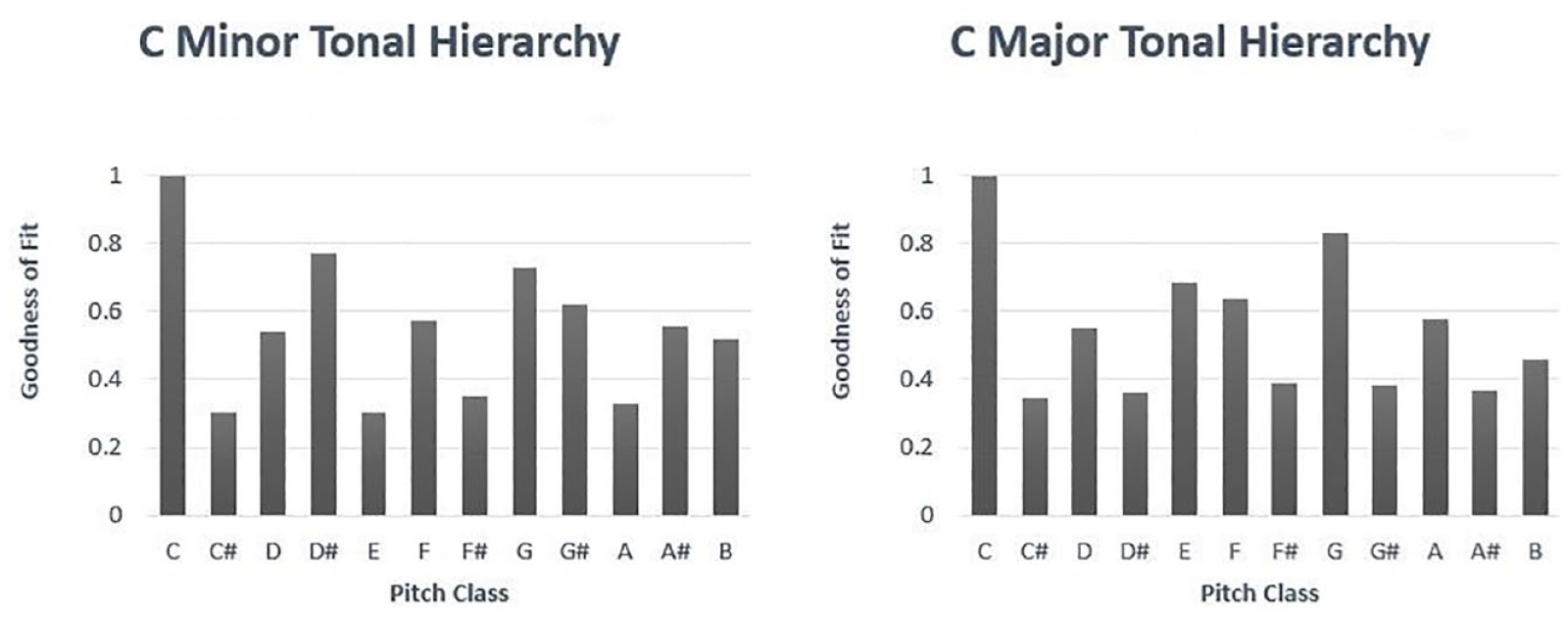
Key profiles for C major and C minor.

The Krumhansl–Schmuckler algorithm measures the number of times a pitch class occurs in a segment and the duration of each occurrence. This approach can overemphasize repeated notes. Consider a segment consisting of a C major triad followed by a series of repeated Es. The system would presumably favor E minor in this case rather than C major, the correct choice. Temperley (2001) suggests a modification (the flat input-weighted key method) where the 12-bin chroma vectors derived from the excerpt would simply use 1 to signify the presence and 0 the absence of each pitch class. The algorithm would use the same correlation-based procedure, again using the weighted key profiles illustrated above. This method goes some way toward solving the problem but may be suboptimal in the context of longer excerpts.

Further key profiles have been proposed since those derived from Krumhansl and Kessler’s probe-tone experiment. Aarden (2003) calculated pitch class distributions from a collection of songs from the Essen folksong collection. Bellmann (2006) derived a model from Budge’s (1943) study of the frequencies of chords used in the works of 18th- and 19th-century composers. Albrecht and Shanahan (2013) trained a key profile using 982 works from the Humdrum database. Temperley (2007) created a key profile by analyzing 46 short harmonic excerpts selected from the textbook of Kostka et al. (1994). Sapp (2011) suggested simple weightings (2 for tonic and dominant, 1 for other diatonic pitch classes, and 0 for non-diatonic pitch classes). These studies offer unique perspectives on modeling pitch class distributions, but—as observed by Sapp (2011)—each model has the potential for misclassification; for example, if Krumhansl and Kessler’s weights are used, the dominant is likely to be identified as the tonic.

All the key profiles described above share the same structure of 12-element vectors, each corresponding to the weight of a pitch class. The Spiral Array (Chew, 2002) is an alternative structure for defining key profiles, a model created in the form of a three-dimensional spiral by rolling up the Harmonic Network, or Tonnetz, described in a range of contexts by Cohn (1997, 1998), Lewin (2007), Longuet-Higgins (1987), and Longuet-Higgins and Steedman (1971). In this three-dimensional space, pitch classes correspond to coordinates on the spiral. The three pitch classes of a triad therefore form a triangle representing chord profiles. Finally, tonic, dominant, and subdominant chord profiles are mapped onto trios of triangles representing key profiles. It is thus possible to identify the key closest to the coordinate representing the aggregate of all the pitch classes in the section, each weighted by their total duration in that section. Chew (2002) examines each possible section of every given excerpt exhaustively, albeit with slight optimizations, to determine the optimal key boundaries. This method of exhaustive examination mirrors our approach of identifying sections in different keys.

The Krumhansl–Schmuckler key-finding algorithm was initially used for global key detection, although there were variations in the ways in which it was used. For example, Krumhansl (1990) considered the first four notes of each of the 48 preludes of Bach’s Well-Tempered Clavier, while Albrecht and Shanahan (2013) used the first and last eight measures of each piece in their dataset. Most such attempts to predict global key understandably aimed to disregard ambiguous or modulating passages. This made it difficult to identify such passages, which are considered “a vital part of tonal music” (Temperley, 2001, p. 187). Temperley proposed dividing an excerpt into segments of arbitrary length, usually less than a second, whereby each segment would be assigned a key based on its local content. Sapp (2005) applied this approach to excerpts from classical music by experimenting with a variety of segment lengths and reported the resulting local key outputs. This produced a visualization for each excerpt in the form of a two-dimensional keyscape in which the sizes of segments increase and the number of segments decrease toward the top of the visualization. Global key is thus indicated at the very top of the keyscape, with lower sections indicating local key content. Although this visualization displays an approximate estimate of modulating passages, it does not indicate definite key boundaries. The task of developing a method for automatic local key detection, via the use of explicit segmentation and labeling, remained to be carried out. As can be observed in the work of Sapp (2005), smaller segment sizes produce frequent and unwarranted modulations. Anticipating these issues, Temperley (2002) suggested penalties if the key of one segment differed from that of the previous segment. These ideas triggered further research on detecting local key accurately.

One important approach to improving the accuracy of local key detection builds on the probabilistic approach of Temperley (2000) by representing the problem as a hidden Markov model (HMM). HMM states correspond to keys; HMM observations correspond to the distributions of pitch classes in each segment of a piece, and emission probability distributions correspond to the key profiles described above. Transition probabilities from one state to another differ across studies. For example, Cho and Bello (2014) employ a uniform probability distribution except for notably high self-transition probabilities, while López et al. (2019) introduced a key distance metric to compute transition probabilities. Here, López et al. separated the 24 keys into nine distinct groups, formed based on their Euclidean distance from a reference point on a matrix of neighboring keys. Each group was sequentially further away from the reference point, and the distance from one group to another was controlled by a ratio parameter. Once the parameters of an HMM have been defined, Viterbi decoding is used to predict a key label for every segment. These labels denote the local key output (Chai & Vercoe, 2005; López et al., 2019; Mearns et al., 2011; Schreiber et al., 2020; Weiß et al., 2020).

Another important approach to local key finding involves deep learning techniques (Schreiber et al., 2020; Schreiber & Müller, 2019). Weiß et al. (2020) compared approaches to local key prediction based on HMMs and neural networks. These approaches were evaluated using three different sets of annotations, each prepared by a different annotator. The objective of using multiple sets of annotations was to not only reveal variations among annotators but also to assess the adaptability of their models to different annotators’ biases. They concluded that their convolutional neural network (CNN) produces results similar to those produced by their version of an HMM, although it appears to be better at mimicking the subjective decisions of specific annotators. Weiß et al. attribute this to the tendency of neural network models to overfit to certain datasets and annotation styles, thus producing inaccurate predictions, while occasionally characterizing misclassifications as non-musical, a rarity in HMM systems.

Our technical approach was inspired, in part, by a technique described in the machine-learning literature and referred to by Rifkin and Lippert (2007) as regularization, whereby the level of complexity of the hypothesis influences the quality of prediction as the result of overfitting. Supervised machine learning involves labeling a dataset, providing a set of hypotheses that map each row of data to a label, and determining the hypothesis that has the best predictive accuracy for new data by optimizing its fit to the dataset provided (i.e., the training data). The selection of the hypothesis set is crucial. A smaller hypothesis set consisting of relatively simple models might underfit (i.e., fail to capture) the underlying relationship between the hypothesis due to bias error, whereas a larger hypothesis set consisting of more complex models might overfit (i.e., capture noise, or meaningless patterns in) the training data. Regularization addresses this issue by adding an adjustable penalty term based on the complexity of the model to the objective function for the best fit, thereby favoring less complex models.

Method

Technical approach and implementation

Our approach to detecting the key of a segment of music diverges from conventional sequential methods for local key detection such as HMM, which primarily consider the content of the segment in the context of the key that was assigned to the previous segment. By contrast, our method takes into consideration the measures that both precede and succeed the segment, simultaneously. In this section, we show how this method is implemented in the case of a single musical excerpt in the form of quantized MIDI data.

We divide the excerpt into segments according to the tempo and time signature information contained in the MIDI data such that every segment consists of a measure.

We compute the correlation between each measure and every key.

We analyze individual measures to produce a comprehensive local key scheme. We assign each measure to a key according not only to the content of the measure itself but also that of the measures that precede and follow it. Using a novel regularization algorithm, we divide all the measures into a series of sections, each one in a single key.

We compared our results with those of an HMM-based approach proposed by López et al. (2019). We did not, however, conduct a similar comparison with the results of deep learning methods, which have been reported to achieve similar performance levels, as discussed in the Related work section of this article (Weiß et al., 2020). Rather, we collaborated with two musical experts to create ground truth annotations. We describe this in detail in the Dataset and evaluation metrics section as annotations are crucial for assessing the performance of both methods.

We computed pitch class vectors based on the total duration of each pitch class. We considered and discarded other metrics, as described in the Discussion. We adapted the key profiles from the work of Krumhansl and Kessler’s (1982) with slight modifications, especially for non-diatonic pitch classes, and for the minor mode, natural and raised 7th pitch classes. We modified the key profiles through the application of simulated annealing, a well-known probabilistic optimization technique (Rutenbar, 1989). The main reason for these adjustments was to account for the diversity of the dataset (see Appendix 1). The implications of such modifications, coupled with the nature of the dataset, are further explained in the Discussion.

We were able to compute the correlation between each measure and every key, not by calculating Euclidean distance or Pearson correlations, but by matching pitch class vectors with key profiles, employing a series of dot products, to obtain an $M \times N$ structure whereby M represents the total number of measures in the excerpt and N represents the total number of possible keys, 12 major and 12 minor.

Use of regularization to identify subsections

The regularization process begins with individual measures and the values of their correlations with every key. The objective is to group them into a set of consecutive measures or subsection, with a single key assigned to each. Individual measures in a subsection do not need to have a perfect correlation with the key assigned to the subsection as a whole. To form these subsections, we undertake a comprehensive exploration of all possible combinations of consecutive measures before selecting the most appropriate combinations based on their quality of fit. This exploration involves calculating a cost for each combination. This yields an optimization problem, whereby we aim to minimize the total cost. Regularization plays a central role in the process of optimization because it enables us to modify the cost function by introducing a penalty term to reduce overfitting. In this context, overfitting refers to the possibility of identifying an excessive number of subsections erroneously implying frequent modulations.

In the remainder of this section, we use an integer-encoding convention to represent pitch classes and keys such that major keys are indexed from 0 to 11, with C major starting at 0, while minor keys are indexed from 12 to 23, with C minor starting at 12. Pitch classes are indexed from 0 to 11, with C as the starting pitch class.

The components of our model are as follows:

$k = 0, 1, 2, \dots, 23$ is the key index.

$P_{k} = {p_{0}, p_{1}, \dots, p_{11}}$ is the key profile of key k.

$m = 1, 2, \dots, M$ is the measure index, where M is the number of measures in the excerpt.

$D_{m} = {d_{0}, d_{1}, \dots, d_{11}}$ is the pitch class/chroma vector of measure m.

$C (m, k) = D_{m} * P_{k}$ is the correlation value for measure m and key k.

$L (m, k) = 1 - C (m, k)$ is the loss function for measure m and key k.

Given an excerpt with M measures, a potential clustering of the set of measures into n subsections can be represented using a set of indices $S = {s_{1}, s_{2}, \dots, s_{n}, s_{n + 1}}$ , where:

$s_{i}, 1 \leq i \leq n$ corresponds to the first measure of the i th subsection.

$s_{n + 1} = M + 1$ indicates the end of the piece for convenience.

Whenever S is updated, it is re-sorted and any duplicates are removed.

To find the key $k_{i}$ for each subsection i, which is the key that yields the maximum correlation we use the following equation:

k_{i} = a r g m i n_{k} (\sum_{m = s_{i}}^{s_{i + 1} - 1} L (m, k))

(1)

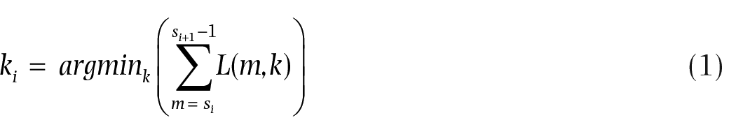
After obtaining $k_{i}$ , we can compute its associated cost $p_{i}$ as:

p_{i} = \sum_{m = s_{i}}^{s_{i + 1} - 1} L (m, k_{i})

(2)

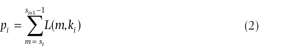
With these subsection costs, we calculate the cost for the entire piece using the regularization function:

R (S) = (\sum_{i = 1}^{| S | - 1} p_{i}) + λ * {(| S | - 2)}^{2} / M

(3)

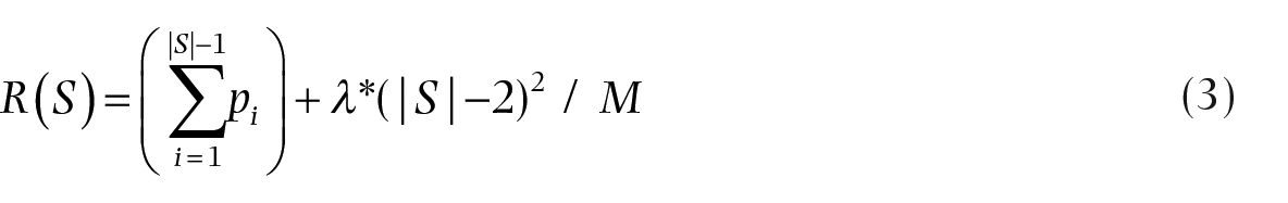
Here, λ is a weight applied to the subsection penalty that can be tuned to improve results.

The regularization function serves as the basis for our algorithm, which aims to discover a partitioning of the piece that minimizes $R (S)$ . Evaluating every possible partitioning of the piece into subsections would be computationally prohibitive due to its exponential nature. Instead, we employ a top-down greedy algorithm as outlined below:

1. Let $S = {s_{1}, s_{2}} = {1, M + 1}$ .

2. For each subsection start index $s_{t} \in S$ , $t = 1, 2, \dots, | S |$ :

a. For each pair of indices $s_{i}$ and $s_{j}$ , $s_{t} \leq s_{i} < s_{j} \leq s_{t + 1}$ :

i. Insert $s_{i}$ and $s_{j}$ into S to construct $S^{'}$ .

ii. Find the key k for measures between $s_{i}$ and $s_{j} - 1$ .

iii. If k differs from the key assigned in the previous iteration for measures between $s_{i}$ and $s_{j}$ , calculate the new cost $R (S^{'})$ . Otherwise, continue to the next iteration without recalculating $R (S^{'})$ (see “-skipped-” rows in illustration below).

3. Select the $S^{'}$ that results in the lowest $R (S^{'})$ in step 2 as a candidate.

4. If $R (S^{'})$ is not less than $R (S)$ , a minimum for equation (3) is reached, conclude the process with S as the final set of subsections. Otherwise, replace S with $S^{'}$ and return to step 2.

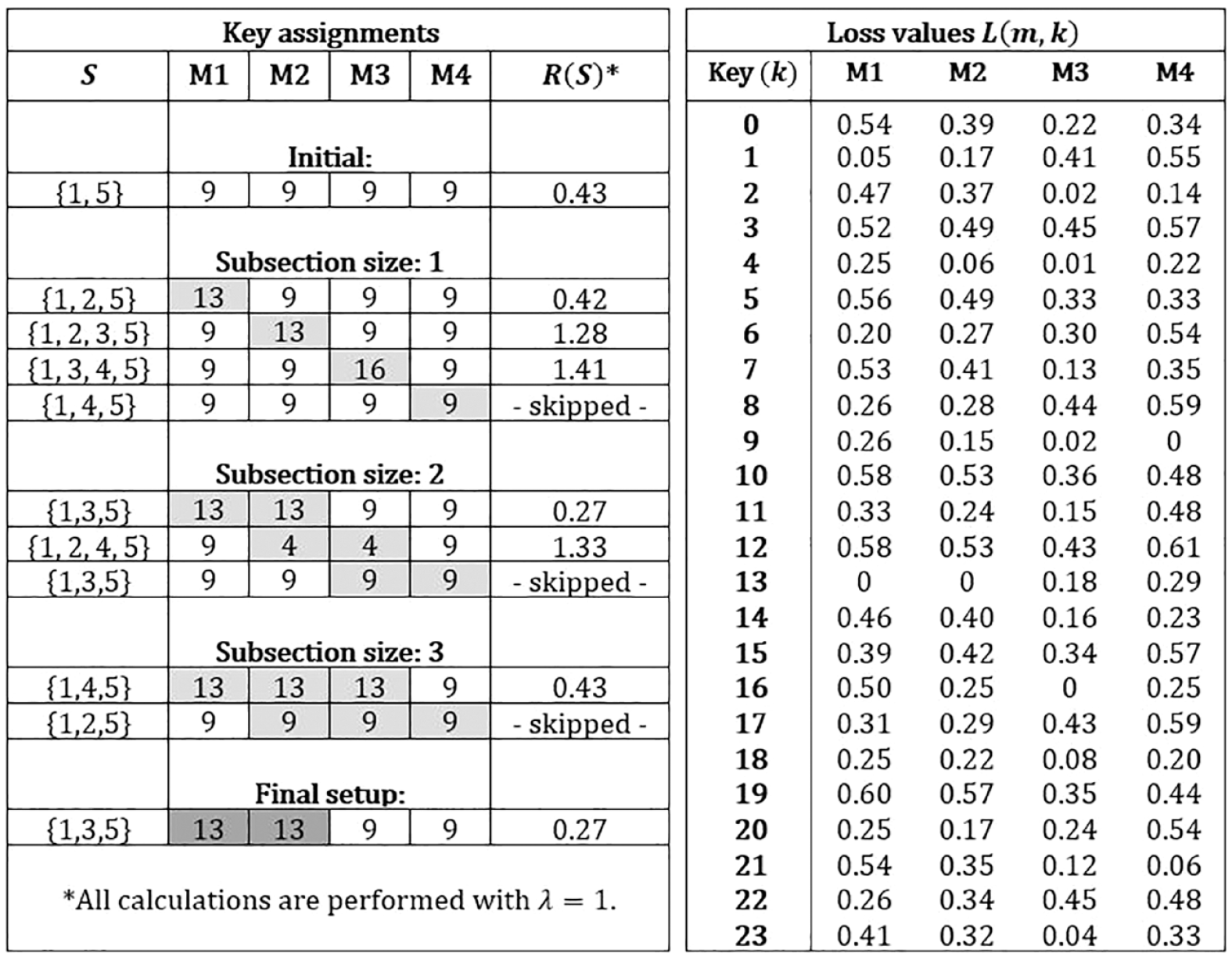
Figure 2 illustrates the calculation process of $R (S)$ for one step for an imaginary 4-measure excerpt.

Figure 2.

One-step demonstration of the regularization algorithm.

We previously argued that our algorithm is adaptable to audio data, provided that pitch class distributions are sufficiently accurate. To demonstrate this claim, we conducted an experiment with studio recordings of two songs from our MIDI dataset: Every Breath You Take (The Police, 1983) and Take My Breath Away (Berlin, 1986) (see Appendix 1 for the complete list). We extracted chroma vectors for each short-time Fourier transform (STFT) frame using the Chroma Toolbox for MATLAB (Müller & Ewert, 2011). Then, we manually formed $D_{m}$ chroma vectors per measure by averaging chroma vectors from those frames that corresponded to specific measures. Finally, we proceeded with the remaining computations, following the methodology described earlier.

Our algorithm suggested identical and correct assignments for both the MIDI and audio versions of Every Breath You Take (The Police, 1983). However, it should be noted that the algorithm interpreted the modulating section as being one measure longer than intended for the MIDI version, as indicated in Figure 3. This discrepancy resulted from our imprecision when converting temporal MIDI messages to measure onsets/offsets in seconds. This led to a slight reduction in accuracy from 100% to 98.9%.

Figure 3.

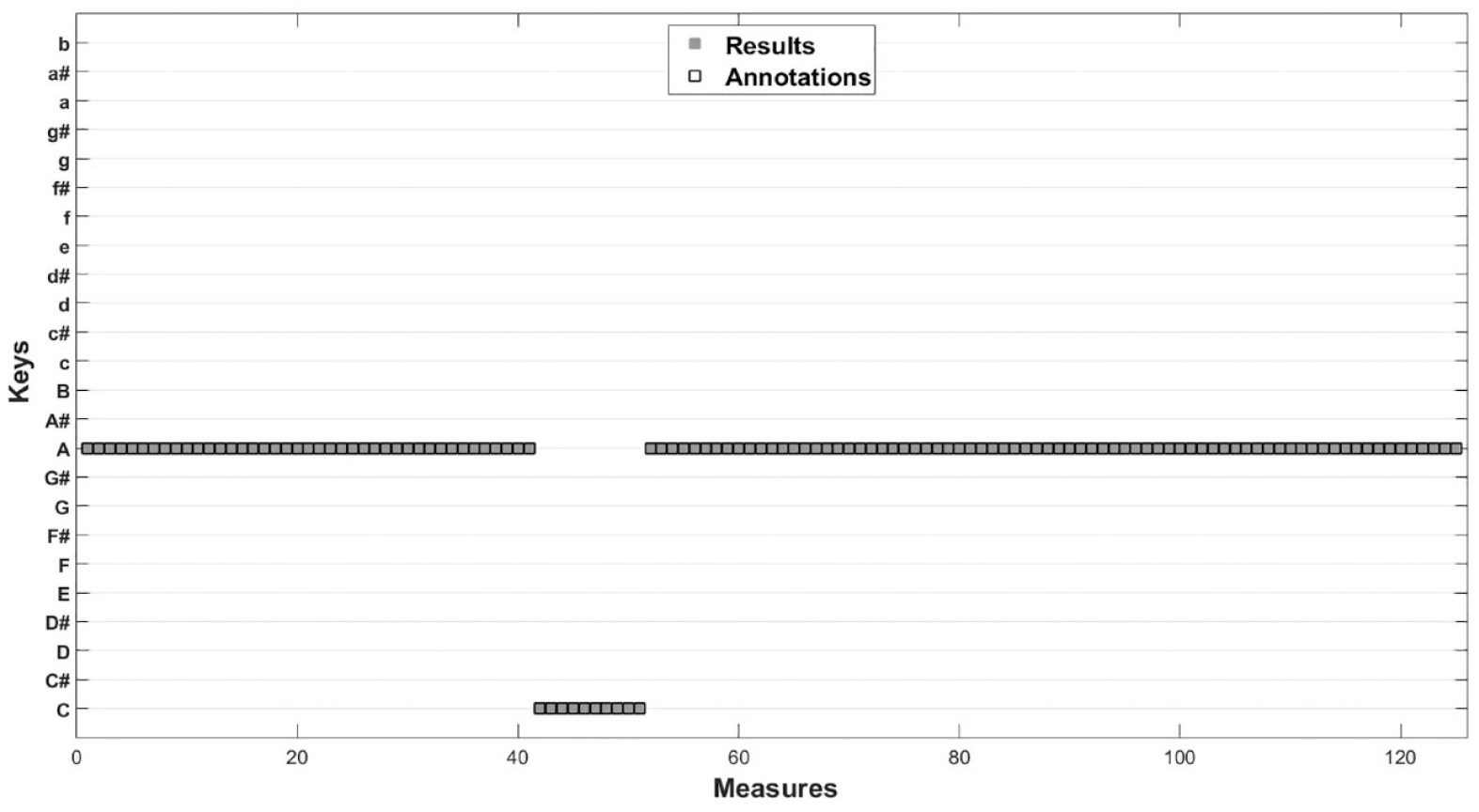
Results of the regularization algorithm applied to Every Breath You Take (The Police, 1983) in wave file format.

Our algorithm performed with near-perfect accuracy in that it produced results for the audio version of Take My Breath Away (Berlin, 1986) that were almost exactly the same as the annotations, as shown in Figure 4. The only discrepancy between the results of the algorithm and the annotations was related to a single measure, the one in which the modulation first occurs (often referred to as the pivot measure), in this case measure 69. The algorithm assigned it to B major, which would have made sense if the measure were considered in isolation. The annotators regarded it as the final measure of a multiple-measure phrase, however, and therefore chose to identify it as belonging to the preceding section. The algorithm performed with considerably less accuracy (66.9%) when applied to the MIDI version of the song, incorrectly assigning F# major to the second section of the song. This was because the MIDI version was poorly transcribed and included lengthy C# notes.

Figure 4.

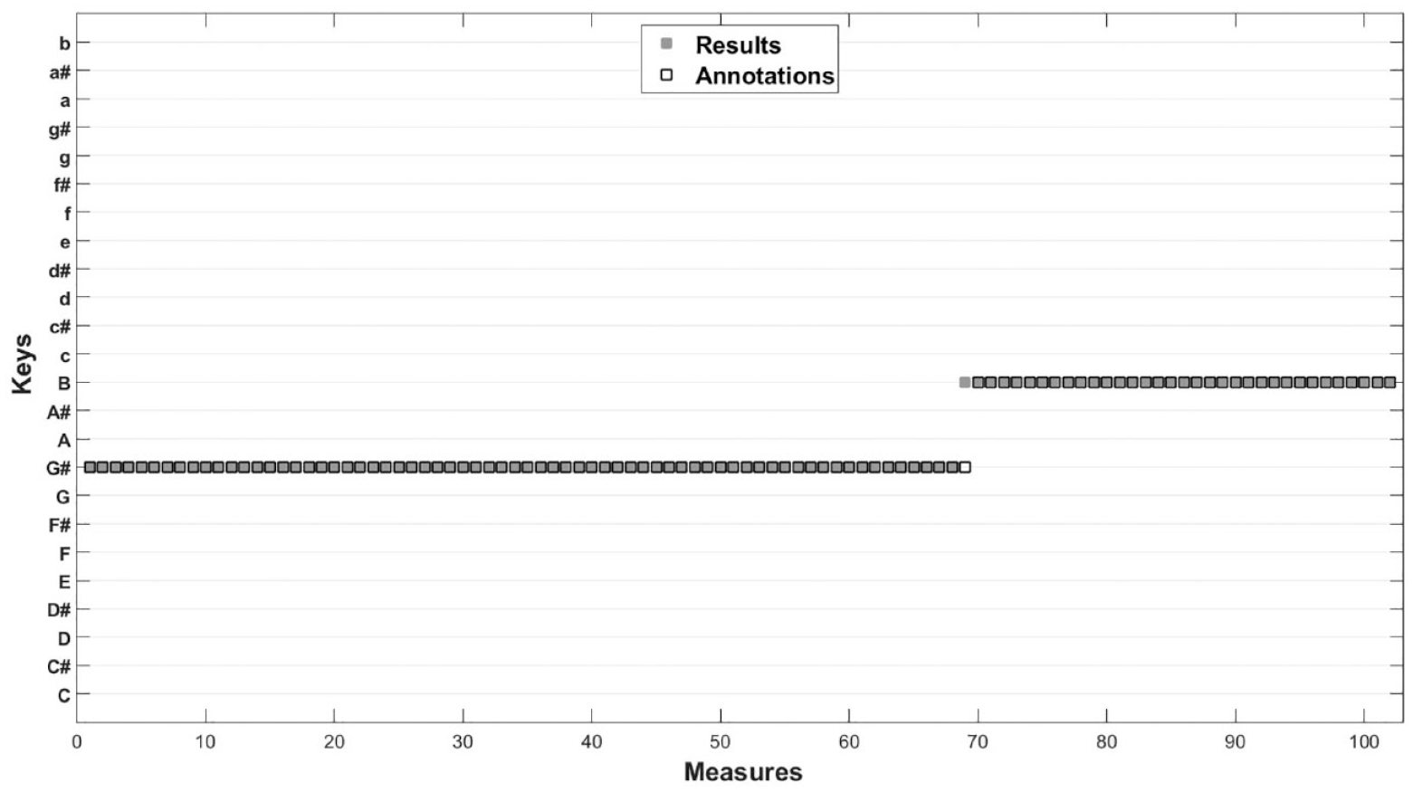
Results of the regularization algorithm applied to Take My Breath Away (Berlin, 1986) in wave file format.

HMM

To assess the performance of the regularization algorithm, we implemented one of the best-performing approaches to local key detection in the form of an HMM. We adapted the approach proposed by López et al. (2019), with a ratio parameter of 6, using Temperley’s key profile (2007) derived from the analysis of excerpts selected from Kostka et al.’s textbook (1994) for major keys and Sapp’s simple weights (2011) for minor keys. We selected these parameters through an optimization process involving all well-known key profiles and a large grid of values for the ratio parameter.

Dataset

We used the Lakh MIDI Dataset (Raffel, 2016) to test our method, limiting our random selection to 80 pieces in a variety of genres and levels of complexity (refer to Appendix 1 for details) because of the time required to annotate each piece by hand. We pre-processed the pieces by removing percussion tracks, normalizing the durations of pitches where necessary (some long notes toward the end of the piece had been overlooked), and eliminating silences at the start of each piece.

Local key detection is inherently challenging and often ambiguous (Weiß et al., 2020). Modulations are often developed gradually over time, making it difficult to pinpoint precise key section boundaries. Furthermore, certain keys such as relative, parallel, or fifth-related keys are closely related and share a large portion of their respective diatonic scales. Moreover, the relationship between the local content of a modulating passage and its intended key might be vague.

This ambiguity warranted annotations from multiple annotators with musical expertise. The first author and two musical experts, each possessing at least five years of formal musical training, labeled each measure independently. They agreed unanimously on 85% of the annotations (Fleiss’ k = .8788), and resolved disagreements in 11% of all cases via a two-to-one majority voting, and 4% of all cases via discussion and eventual consensus. The annotators did not consider modal structures and grouped the annotations into major and minor keys (see Pitch class vectors in the Discussion).

Evaluation metrics

We used different metrics to evaluate each of the approaches:

Perfect match: assignment of measure to key, scoring 1 for correct and 0 for incorrect;

Distance-based: assignment of each measure to key, scoring between 0 (representing the ground truth as determined by the annotations) and 1 according to the distance between the ground truth and the key assigned by the algorithm or HMM, calculated on the basis of a nested circle of fifths, adapted from the work of Bello and Pickens (2005);

MIREX score representing a simplified calculation of distance between two keys, scoring 1 for correct, 0.5 for incorrect at the distance of a perfect fifth, 0.3 for incorrect (relative major or minor), 0.2 for incorrect (parallel major or minor), and 0 for incorrect for any other reason.

We scored each measure of each piece using all three metrics and then calculated the mean of the three scores for each measure. Finally, we calculated the mean of scores across all the pieces in the dataset for each of the three metrics separately.

Results

We applied each of the metrics to our dataset and report accuracy results for each metric for each piece in Appendix 1. These are illustrated in box-and-whisker graphs comparing error percentages in Figure 5.

Figure 5.

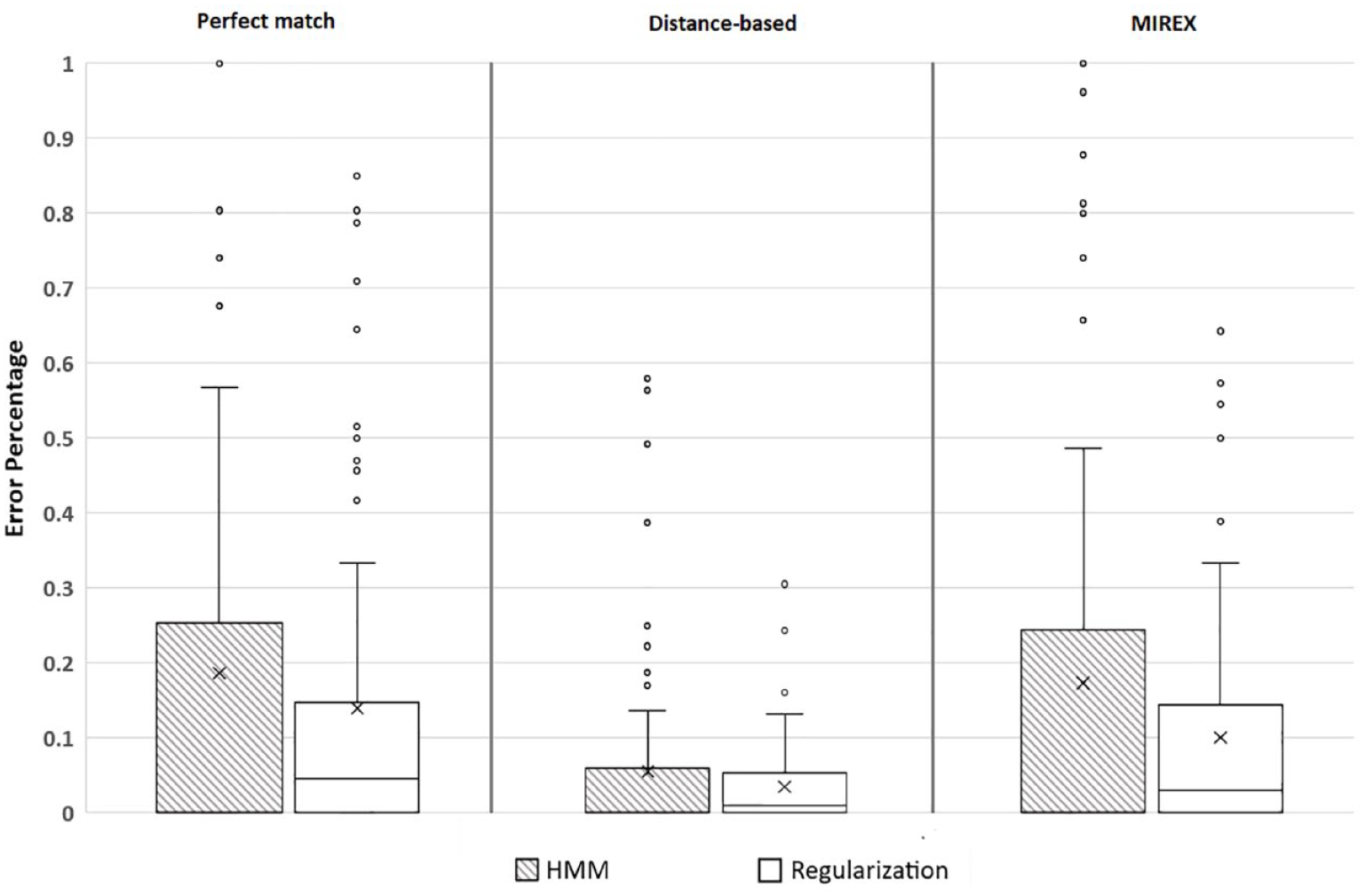
Comparison of error percentages for each of the three metrics and the regularization algorithm.

We carried out three independent-samples t-tests to compare the results of our regularization algorithm with those of the perfect-match, distance-based, and MIREX metric. There was a significant difference between our results and those of the HMM using the MIREX metric (t₁₅₈ = 1.95, p = .026, d = 0.30), such that our results were more accurate (M = 0.899, SD = 0.157) than those of the HMM (M = 0.826, SD = 0.292), but there were no significant differences between our results and those of the HMM according to the perfect-match or distance-based metrics.

Discussion

The HMM was 100% accurate for 41 of the 80 pieces but unlike regularization the HMM produced a large proportion of results that were less than 35% accurate. This is because the HMM assigns key to measure on the basis only of the previous measure, and if the wrong key has been assigned to the previous measure, then this will affect the key assigned to the measure in question (as shown by the larger interquartile ranges and more extreme scores for the HMM in Figure 5). Using the MIREX metric for the HMM, our algorithm performed significantly better because it was less likely to incorrectly identify a measure as containing a modulation, although it also failed to identify some measures in which there were brief modulations. When our algorithm assigned the wrong key, it was likely to be closer to the ground truth key, typically at the distance of a perfect fifth or a relative major or minor, than the wrong key assigned by the HMM.

Input media format

The process of segmenting a MIDI file into measures makes use of temporal information encoded in this format. However, it is important to acknowledge that this temporal information can be imprecise and misleading. Measures, and the notes within them, may therefore be identified inaccurately. They are likely to be identified with greater accuracy if the researcher adheres closely to MIDI specifications.

In contrast, segmenting an audio excerpt into measures involves extracting temporal information from the audio signal. The identification of segment onsets and offsets can be affected, however, by the use of tempo- and beat-tracking techniques (Ellis & Poliner, 2007; Schreiber & Müller, 2019). This can be avoided by segmenting the excerpt into frames of fixed duration instead of measures, and this method is commonly preferred method in audio-based musical content analysis. As described in the Method section, we merged STFT frames into their respective measures, manually, to create a basis for comparison between the results obtained from pieces in MIDI and audio formats. This type of segmentation is more musical and produces data that are more suitable for interpretation, which is crucial for creating a better model of music perception.

Pitch class vectors

We considered three ways of formulating initial pitch class vectors: counting the occurrences of pitch classes, computing their total duration, and taking the flat-input/weighted-key approach (Temperley, 2001). Computing total duration yielded the most accurate results for our dataset. Nevertheless, alternative formulations combining other methods such as velocity or octave range are possible, as discussed by Chew (2002). How pitch class vectors are formulated can affect results, however. For example, counting the occurrences of pitch classes in Godzilla (Blue Öyster Cult, 1977) produced a perfect-match accuracy score of 0%. The flat-input/weighted key approach for the same piece produced a score of 15.5% and total duration a score of 87.5%. This should be considered in future research.

Parameter tuning

The scalar λ is directly and proportionally linked to the subsection penalty. Therefore, lower λ values encourage and higher λ values discourage the formation of subsections. A constant λ implies that the algorithm cannot perform equally well on pieces with varying levels of complexity in terms of modulations. We hypothesize that a system that can adapt to different complexity levels by tuning λ based on factors that are considered to be influential should allow for further improvements. In our testing, we identified genre as the most influential factor for modulations, but a thorough analysis could reveal further alternatives. Machine learning methods should be especially valuable for discovering such features.

Modality and key profiles

Our dataset contains pieces from a variety of genres, including pop and rock. We concede that modal harmonic structures, often present within these genres (Moore, 1992, 1995), are not strictly compatible with Krumhansl and Kessler’s key profiles, which are originally derived from common-practice period music. Thus, accuracy for pieces that exhibit modality may benefit from the crafting of key profiles tailored for modal structures, irrespective of the algorithm. However, we do not believe that such a modification alone would improve the overall performance of our algorithm for the dataset, given its substantial content of music from the common-practice period. Finally, the computation of pitch class vectors in modal pieces was beyond the scope of the research reported in this article. We therefore opted to group minor and major modes separately to illustrate the operation of the regularization algorithm and left modal key analysis and key-profile tuning for a future investigation.

Conclusions and future work

In this article, we introduced a novel regularization algorithm for local key detection and compared it to an HMM adapted from the work of López et al. (2019). Our regularization algorithm yielded a statistically significant increase in overall predictive accuracy. Given the diversity of our dataset, the results suggest that achieving universal adaptability for a local key detection algorithm may be unfeasible. Instead, it might be more practical to create datasets tailored to specific characteristics such as genre, allowing for the calibration of any parameter based on accuracy results obtained from each dataset. In future, we plan to explore the avenues for optimizing the use of the algorithm discussed above by revising the dataset in such a way that it consists of pieces in a narrower range of genres.

Footnotes

Appendix 1 Funding

The authors received no financial support for the research, authorship, and/or publication of this article.

ORCID iD

Çınar Gedizlioğlu

References

Aarden

(2003). Dynamic melodic expectancy [Doctoral dissertation, The Ohio State University]. OhioLINK Electronic Theses and Dissertations Center. http://rave.ohiolink.edu/etdc/view?acc_num=osu1060969388

Albrecht

Shanahan

(2013). The use of large corpora to train a new type of key-finding algorithm: An improved treatment of the minor mode. Music Perception, 31(1), 59–67. https://doi.org/10.1525/MP.2013.31.1.59

Bellmann

(2006). About the determination of key of a musical excerpt. In Kronland-Martinet

Ystad

Voinier

(Eds.), Lecture notes in computer science: Vol. 3902. Computer music modeling and retrieval (pp. 76–91). Springer. https://doi.org/10.1007/11751069_7

Bello

J. P.

Pickens

(2005). A robust mid-level representation for harmonic content in music signals. In Proceedings of the 6th International Conference on Music Information Retrieval (pp. 304–311). University of London.

Berlin. (1986). Take my breath away [Song]. On Count three & pray. Columbia Records.

Birajdar

G. K.

Patil

M. D.

(2020). Speech/music classification using visual and spectral chromagram features. Journal of Ambient Intelligence and Humanized Computing, 11(1), 329–347. https://doi.org/10.1007/s12652-019-01303-4

Blue Öyster Cult. (1977). Godzilla [Song]. On Spectres. Columbia Records.

Budge

(1943). A study of chord frequencies based on the music of representative composers of the eighteenth and nineteenth centuries [Unpublished doctoral dissertation]. Columbia University Teacher’s College, New York.

Chai

Vercoe

(2005). Detection of key change in classical piano music. In Proceedings of the 6th International Conference on Music Information Retrieval (pp. 468–473). University of London.

10.

Chew

(2002). The spiral array: An algorithm for determining key boundaries. In Anagnostopoulou

Ferrand

Smaill

(Eds.), Lecture notes in computer science: Vol. 2445. Music and artificial intelligence (pp. 18–31). Springer-Verlag. https://doi.org/10.1007/3-540-45722-4_4

11.

Cho

Bello

J. P.

(2014). On the relative importance of individual components of chord recognition systems. IEEE Transactions on Audio, Speech and Language Processing, 22(2), 477–492. https://doi.org/10.1109/TASLP.2013.2295926

12.

Cohn

(1997). Neo-Riemannian operations, parsimonious trichords, and their “Tonnetz” representations. Journal of Music Theory, 41(1), 1–66. https://doi.org/10.2307/843761

13.

Cohn

(1998). Introduction to neo-Riemannian theory: A survey and a historical perspective. Journal of Music Theory, 42(2), 167–180. https://doi.org/10.2307/843871

14.

Downie

S. J.

Ehmann

A. F.

Lee

J. H.

(2008). The Music Information Retrieval Evaluation eXchange (MIREX): Community-led formal evaluations. In Opas-Hänninen

L. L.

Jokelainen

Juuso

Seppänen

(Eds.), Digital humanities 2008: Book of abstracts (pp. 239–241). English Philology, University of Oulu.

15.

Ellis

D. P. W.

Poliner

G. E.

(2007). Identifying “cover songs” with chroma features and dynamic programming beat tracking. Proceedings of the 2007 IEEE International Conference on Acoustics, Speech and Signal Processing, 4, 1429–1432. https://doi.org/10.1109/ICASSP.2007.367348

16.

Fujishima

(1999). Realtime chord recognition of musical sound: A system using common lisp music. Proceedings of the International Computer Music Conference, ICMC, 1999, 464–467. http://quod.lib.umich.edu/i/icmc/bbp2372.1999

17.

Kostka

Payne

Schindler

(1994). Tonal harmony: With an introduction to twentieth-century music (3rd ed.). McGraw-Hill Higher Education.

18.

Krumhansl

C. L.

(1990). Cognitive foundations of musical pitch. Oxford University Press.

19.

Krumhansl

C. L.

Kessler

E. J.

(1982). Tracing the dynamic changes in perceived tonal organisation in a spatial representation of musical keys. Psychological Review, 89(4), 334–368. https://doi.org/10.1037/0033-295X.89.4.334

20.

Lewin

(2007). Generalized musical intervals and transformations. Oxford University Press. https://doi.org/10.1093/acprof:oso/9780195317138.001.0001

21.

Longuet-Higgins

H. C.

(1987). Mental processes: Studies in cognitive science. MIT Press.

22.

Longuet-Higgins

H. C.

Steedman

(1971). On interpreting Bach. In Meltzer

Michie

(Eds.), Machine intelligence (Vol. 6, pp. 221–243). Edinburgh University Press.

23.

López

N. N.

Arthur

Fujinaga

(2019). Key-finding based on a hidden Markov model and key profiles. In DLfM ’19: Proceedings of the 6th International Conference on Digital Libraries for Musicology (pp. 33–37). Association for Computing Machinery. https://doi.org/10.1145/3358664.3358675

24.

Luque-Fernandez

M. A.

Schomaker

Rachet

Schnitzer

M. E.

(2018). Targeted maximum likelihood estimation for a binary treatment: A tutorial. Statistics in Medicine, 37(16), 2530–2546. https://doi.org/10.1002/sim.7628

25.

Mearns

Benetos

Dixon

(2011). Automatically detecting key modulations in J.S. Bach chorale recordings. Proceedings of the 8th Sound and Music Computing Conference, 37(9), 1591–1601. https://doi.org/10.5281/zenodo.1400730

26.

Moore

(1992). Patterns of harmony. Popular Music, 11(1), 73–106. https://doi.org/10.1017/S0261143000004852

27.

Moore

(1995). The so-called “flattened seventh” in rock. Popular Music, 14(2), 185–201. https://doi.org/10.1017/S0261143000007431

28.

Müller

Ewert

(2011). Chroma toolbox: Matlab implementations for extracting variants of chroma-based audio features. In Proceedings of the 12th International Society for Music Information Retrieval Conference (pp. 215–220). University of Miami.

29.

Myung

I. J.

(2003). Tutorial on maximum likelihood estimation. Journal of Mathematical Psychology, 47(1), 90–100. https://doi.org/10.1016/S0022-2496(02)00028-7

30.

Pauwels

Martens

J.-P.

(2010, May 1). Integrating musicological knowledge into a probabilistic framework for chord and key extraction [Conference session]. 128th AES Convention, London. http://www.aes.org/e-lib/browse.cfm?elib=15383

31.

The Police. (1983). Every breath you take [Song]. On Synchronicity. A&M Records.

32.

Raffel

(2016). Learning-based methods for comparing sequences, with applications to audio-to-MIDI alignment and matching [Doctoral dissertation, Columbia University]. Columbia Academic Commons. https://doi.org/10.7916/D8N58MHV

33.

Rifkin

R. M.

Lippert

R. A.

(2007). Value regularization and Fenchel duality. Journal of Machine Learning Research, 8, 441–479.

34.

Rutenbar

R. A.

(1989). Simulated annealing algorithms: An overview. IEEE Circuits and Devices Magazine, 5(1), 19–26. https://doi.org/10.1109/101.17235

35.

Sapp

C. S.

(2005). Visual hierarchical key analysis. Computers in Entertainment, 3(4), 1–19. https://doi.org/10.1145/1095534.1095544

36.

Sapp

C. S.

(2011). Computational methods for the analysis of musical structure [Doctoral dissertation, Stanford University]. Stanford Libraries. http://purl.stanford.edu/br237mp4161

37.

Schreiber

Müller

(2019). Musical tempo and key estimation using convolutional neural networks with directional filters. In Barbancho

Tardón

L. J.

Peinado

Barbancho

A. M.

(Eds.), Proceedings of the 16th Sound & Music Computing Conference, SMC 2019 (pp. 47–54). Zenodo.

38.

Schreiber

Weiß

Müller

(2020). Local key estimation in classical music recordings: A cross-version study on Schubert’s Winterreise. Proceedings of the 2020 IEEE International Conference on Acoustics, Speech, and Signal Processing (pp. 501–505). IEEE. https://doi.org/10.1109/ICASSP40776.2020.9054642

39.

Temperley

(2001). The cognition of basic musical structures. MIT Press. https://doi.org/10.1525/mp.2005.23.2.189

40.

Temperley

(2002). A Bayesian approach to key-finding. In Anagnostopoulou

Ferrand

Smaill

(Eds.), Lecture notes in computer science: Vol. 2445. Music and artificial intelligence (pp. 195–206). Springer-Verlag. https://doi.org/10.1007/3-540-45722-4_18

41.

Temperley

(2007). Music and probability. MIT Press. https://doi.org/10.7551/mitpress/4807.001.0001

42.

Weiß

Schreiber

Muller

(2020). Local key estimation in music recordings: A case study across songs, versions, and annotators. IEEE/ACM Transactions on Audio Speech and Language Processing, 28, 2919–2932. https://doi.org/10.1109/TASLP.2020.3030485

A regularization algorithm for local key detection

Abstract

Keywords

Method

Technical approach and implementation

Use of regularization to identify subsections

HMM

Dataset

Evaluation metrics

Results

Discussion

Input media format

Pitch class vectors

Parameter tuning

Modality and key profiles

Conclusions and future work

Footnotes

Appendix 1

Funding

ORCID iD

References