Sage Journals: Discover world-class research

Abstract

Glioblastoma multiforme is the most common primary brain tumor and is highly lethal. This study aims to figure out signatures for predicting the survival time of patients with glioblastoma multiforme. Clinical information, messenger RNA expression, microRNA expression, and single-nucleotide polymorphism array data of patients with glioblastoma multiforme were retrieved from The Cancer Genome Atlas. Patients were separated into two groups by using 1 year as a cutoff, and a logistic regression model was used to figure out any variables that can predict whether the patient was able to live longer than 1 year. Furthermore, Cox’s model was used to find out features that were correlated with the survival time. Finally, a Cox model integrated the significant clinical variables, messenger RNA expression, microRNA expression, and single-nucleotide polymorphism was built. Although the classification method failed, signatures of clinical features, messenger RNA expression levels, and microRNA expression levels were figured out by using Cox’s model. However, no single-nucleotide polymorphisms related to prognosis were found. The selected clinical features were age at initial diagnosis, Karnofsky score, and race, all of which had been suggested to correlate with survival time. Both of the two significant microRNAs, microRNA-221 and microRNA-222, were targeted to p27^Kip1 protein, which implied the important role of p27^Kip1 on the prognosis of glioblastoma multiforme patients. Our results suggested that survival modeling was more suitable than classification to figure out prognostic biomarkers for patients with glioblastoma multiforme. An integrated model containing clinical features, messenger RNA levels, and microRNA expression levels was built, which has the potential to be used in clinics and thus to improve the survival status of glioblastoma multiforme patients.

Keywords

Glioblastoma multiforme survival analysis Cox’s model logistic regression messenger RNA expression microRNA expression single-nucleotide polymorphism

Introduction

Glioblastoma multiforme (GBM) is the most frequent and the most aggressive primary brain tumor. GBM is classified as a Grade IV astrocytoma, which is the most serious scale.¹ It develops primarily in the cerebral hemispheres but can also develop in other parts of the brain, brainstem, or spinal cord. The current standard of care for GBM patients, including surgical resection, adjuvant radiation therapy, chemotherapy, and the oral alkylating agent temozolomide, elongates the survival time, but the median survival is still only 15 months.² The poor prognosis encourages the researchers to study the methods to improve the survival status of GBM patients. One approach is to find out the prognostic biomarkers, which can be used to figure out the subtype of cancer and give personalized therapy.

There were mainly three different methods to study the prognosis of cancer, that is, classification, survival modeling, and clustering. Considering that this article aimed to find out biomarkers for the prognosis of GBM, clustering is unsuitable because it is commonly used to find out the subtype of cancer. Other two methods, classification and survival modeling, were both used to decide the biomarkers. This study aimed to use classification and survival modeling to find prognostic biomarkers for GBM and build the logistic regression model or Cox’s model which has the potential to be applied in practice.

Methods and materials

TCGA GBM dataset

Clinical information, messenger RNA (mRNA) expression, microRNA (miRNA) expression, and single-nucleotide polymorphism (SNP) array data of patients with GBM were retrieved from The Cancer Genome Atlas (TCGA). This dataset contains 596 patients. Level 3 mRNA expression and miRNA expression data of Agilent expression array will be used to figure out the mRNAs and miRNAs related to patients’ survival. SNP and mutation information are available in the platform of Affymetrix Genome-Wide Human SNP Array 6.0.

Classification

Patients were separated into two groups using 1 year as a cutoff. One group contains patients living longer than 1 year no matter they died or not after 1 year. The other group contains patients who died within 1 year. As a result, patients with censored data less than 1 year were removed from this study. Such filtering left 484 patients, among which mRNA and miRNA expression data were available for 471 and 461 subjects, respectively. The filtered patients were randomly separated into training and testing datasets by a ratio of 8:2.

After filtering, analysis of variance (ANOVA) was used to identify clinical variables that displayed differently in high-risk or low-risk groups. R package limma³ was used to figure out mRNAs and miRNAs which were differentially expressed between the two groups on the training dataset. Two cutoffs, 0.0005 and 0.05, were applied to the raw p value. The different cutoffs were used in order to control the final variables used in the classification models. With these mRNA or miRNA data, logistic regression models were built and tested on the testing dataset. The performances of classification models were shown using the receiver operating characteristic (ROC) curve plots and the heat maps.

Cox’s model

A total of 39 patients without mRNA expression or miRNA expression data were filtered out, and this filtering left 557 patients for analysis. Among these patients, Karnofsky score was unavailable for 137 patients. Each clinical variable was used to build a univariate Cox proportional hazard ratio model.⁴ Patients with unavailable data were excluded. Quantities of interest hazard ratios for linear coefficients were plotted using R package simPH.⁵ Each mRNA or miRNA was fitted to univariate Cox’s model as well.⁴ False discovery rate (FDR) adjustment was carried out on the results of miRNA expression data, and significant miRNAs were selected with a cutoff of 0.05.

Multivariate Cox’s model was built with the expression levels of significant mRNAs or miRNAs based on the training dataset. Patients were separated into high-risk and low-risk groups according to their predicted hazard ratio. In this case, median of the hazard ratio was used as the cutoff, and patients were separated into the high-risk and low-risk groups evenly. The Kaplan–Meier plots and the log rank tests with the high-risk or low-risk groups were carried out on both the training and testing datasets.

SNP and mutations

As described above, patients were arbitrarily separated into two groups using 1 year as the cutoff. The frequencies of genes where any SNP or mutation happened were counted in two groups after silent mutations were removed. Only genes whose SNP or mutation appeared in more than 10% of patients were taken into account. The chi-square test was used to figure out genes that had different occurrences between the two groups.

Within all patients with SNP data, a matrix was built to determine whether each gene had SNP occurred in each patient. Cox’s model was fitted to study whether the occurrence of SNP on one gene would lead to different survival times.

Integrated model

A Cox’s model integrated the clinical variables, mRNA expression, miRNA expression, and SNP identified using the survival modeling was built. A stepwise model selection by the Akaike information criterion (AIC) was carried out to avoid over-fitting. The integrated model was built on the training dataset and was verified on the testing dataset.

Results

Clinical parameters related to prognosis

Two methods were used to identify clinical parameters related to prognosis, that is, classification and the Cox model. The p values of each method were summarized in Table 1. No clinical parameter was significant when ANOVA was carried out on two groups, while the log likelihood test of Cox’s model found that age at initial diagnosis, race, and Karnofsky score were significantly related to survival time.

Table 1.

Possibility that clinical variables were associated with survival time.

	Classification^a	Cox’s model^b
Gender	3.56E-01	2.13E-01
Age at initial diagnosis	1.70E-01	7.77E-16
Race	1.51E-01	2.10E-02
Ethnicity	1.79E-01	9.09E-01
Karnofsky score^c	3.74E-01	3.18E-07

One-way analysis of variance (ANOVA) was used to compare whether these variables were different between the group of patients living longer than 1 year and the group of patients died within 1 year.

These p values were obtained using the log likelihood test of Cox’s model.

Karnofsky score is an index describing patients’ functional impairment. A smaller Karnofsky score means a serious impairment.

The relations between hazard ratio and numeric variable were shown in Figure 1. The younger when the patient is diagnosed with GBM or the larger the Karnofsky score is, the lower the hazard ratio is. These plots showed a 95% (the lightest blue) and 50% (the light blue) probability interval of the simulations.⁵ While the Karnofsky score had a relatively stable 95% probability interval of the simulations, the probability interval of age at initial diagnosis increased dramatically along with the increased age. It suggested that the prognosis of patients with larger age at initial diagnosis was much more changeable than that of younger patients. As a result, it may be more difficult to predict the survival time of older patients and give them personal treatment.

Figure 1.

Quantities of interest hazard ratios for age at initial diagnosis (left) and Karnofsky score (right) from Cox’s model. The 95% and 50% probability intervals of the simulations were shown in different shades of blue. The X-axle represents the patients’ ages at initial diagnosis, and the Y-axle represents the hazard ratio.

Performance of classification

With groups of patients living longer or shorter than 1 year, p values were calculated with R package limma.³ The mRNAs that have p values less than 5.0E-4 were listed in Table 2. Even though the p values of these mRNAs seemed significant, the adjusted p values using the FDR method were larger than 0.05. As a result, considering the total 17,417 mRNAs available, there were no significant mRNAs whose expression levels were different between the two groups.

Table 2.

The p value and FDR of top mRNAs whose expression levels were related to survival time.

	logFC	p value	FDR
IRF7	0.207	3.41E-05	0.401
COG3	0.161	5.24E-05	0.401
DES	0.351	9.45E-05	0.401
C19orf25	0.197	1.22E-04	0.401
ZNF575	0.240	1.26E-04	0.401
OPA3	0.136	1.38E-04	0.401
E4F1	0.137	1.83E-04	0.416
PKN2	0.189	2.47E-04	0.416
CHCHD4	−0.123	2.89E-04	0.416
PARP10	0.230	3.10E-04	0.416
ARTN	0.191	3.49E-04	0.416
UNC93B1	0.224	3.90E-04	0.416
SELV	0.389	4.35E-04	0.416
IFI27	0.379	4.37E-04	0.416

FDR: false discovery rate; mRNA: messenger RNA; FC: fold change.

The ROC plots (Figure 2) and the heat maps (Supplementary Figures 1 and 2) both confirmed that these mRNAs were poor biomarkers for classification. Then, a logistic regression model was built based on the training dataset using these 14 mRNAs and a stepwise model selection was carried out to find a better model with lower AIC. The feature-selected model contained OPA3, PARP10, E4F1, CHCHD4, COG3, UNC93B1, IFI27, and SELV. The ROC plots of these models on training and testing datasets were shown in Figure 2. The area under the curve (AUC) of the training dataset is only 0.71, which suggested that it was not a good model. Moreover, the AUC of the testing dataset was only 0.40, which was even worse than a random model.

Figure 2.

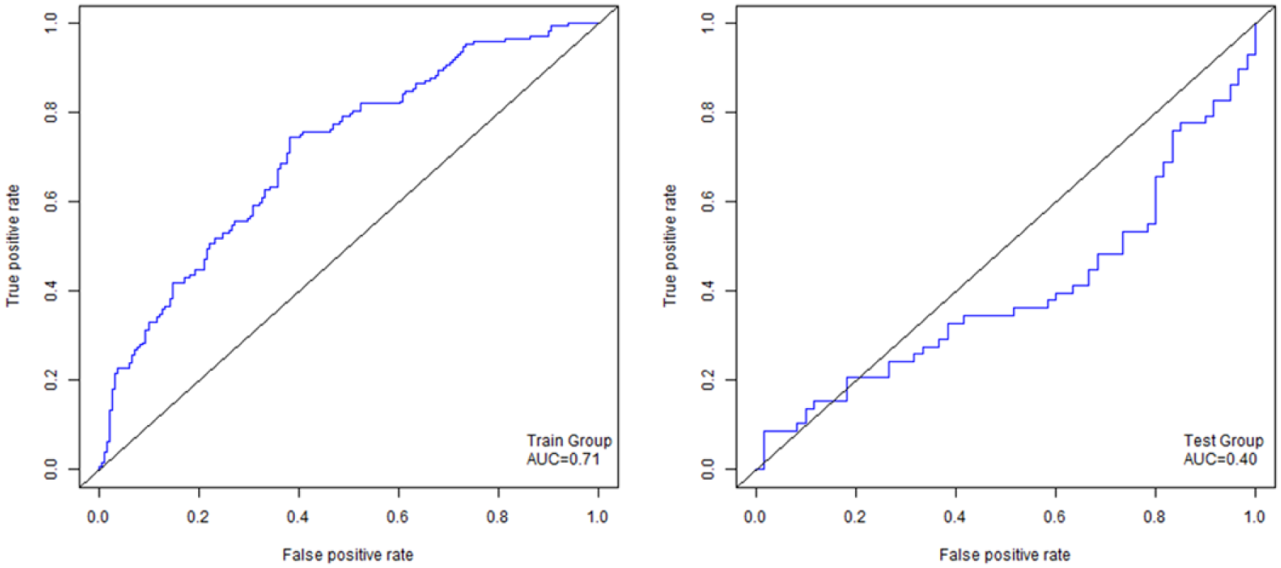
The ROC plot of logistic regression using mRNAs with p value less than 0.001 on both training (left) and testing (right) datasets by classification.

The same analysis was carried out with expression levels of miRNAs. The p values and adjusted p values were shown in Table 3. Similarly, some of miRNAs had p values less than 0.05, but their FDRs were insignificant. The ROC plots (Figure 3) and the heat maps (Supplementary Figures 3 and 4) also suggested that these miRNAs could not be used to classify patients and decide whether they were able to live longer than 1 year.

Table 3.

The p value and FDR of top miRNAs whose expression levels were related to survival time.

	logFC	p value	FDR
hsa-miR-769-5p	0.079	5.01E-03	0.978
hsa-miR-548b	0.015	2.16E-02	0.978
hsa-miR-409-5p	0.041	2.35E-02	0.978
hsa-miR-422b	−0.121	3.13E-02	0.978
hsa-miR-200c	−0.106	3.49E-02	0.978
ebv-miR-BART3-3p	−0.010	3.86E-02	0.978
hsa-miR-597	0.010	3.93E-02	0.978
hsa-miR-550	0.073	4.31E-02	0.978
hsa-miR-199a	−0.210	4.60E-02	0.978

FDR: false discovery rate; miRNA: microRNA.

Figure 3.

The ROC plot of logistic regression using miRNAs with p value less than 0.05 on both training (left) and testing (right) datasets by classification.

Performance of Cox’s model

Univariate Cox’s model was built based on each mRNA or miRNA. Their p values and adjusted p values were summarized in Table 4. The types of mRNA or miRNA were decided by their coefficients. If the mRNA or miRNA had a positive coefficient, the higher expression level it had, the larger the hazard ratio. So it was a risky biomarker. However, it was a protective biomarker.

Table 4.

The p value and FDR of significant mRNAs and miRNAs.

Symbol	p value	FDR	Type
mRNA
RANBP17	1.01E-08	1.75E-04	Protective
KIAA0495	4.02E-07	2.34E-03	Risky
UBE2Z	4.03E-07	2.34E-03	Risky
HPGD	1.15E-06	5.00E-03	Protective
CYB561	2.05E-06	7.16E-03	Risky
CLEC5A	3.60E-06	8.98E-03	Risky
IZUMO1	3.11E-06	8.98E-03	Protective
COL22A1	4.43E-06	9.66E-03	Risky
PDSS1	4.99E-06	9.67E-03	Risky
RAB36	5.68E-06	9.90E-03	Protective
miRNA
hsa-miR-222	1.49E-06	7.95E-04	Risky
hsa-miR-221	2.76E-05	7.37E-03	Risky

FDR: false discovery rate; mRNA: messenger RNA; miRNA: microRNA.

Multivariate Cox’s model was built with the expression levels of significant mRNAs based on the training dataset. Patients were separated into high-risk and low-risk groups according to their predicted hazard ratio. In this case, median of the hazard ratio was used as the cutoff, and patients were separated into the high-risk and low-risk groups evenly. The cutoff can be decided by the specific goal. The Kaplan–Meier plots of high-risk and low-risk groups in both the training and testing datasets were shown in Figure 4. The p value of the log rank test, which measures whether the two or more groups have different survival times, was only 3.0E-11 on the training dataset and 9.7E-03 on the testing dataset. The significant p value on the testing dataset showed that these mRNA signatures were able to separate the patients into high-risk and low-risk groups. But the differences between p values of training and testing datasets might imply that the model was over-fitted.

Figure 4.

The Kaplan–Meier plot using mRNAs with FDR less than 0.01 on both training (left) and testing (right) datasets by Cox’s model.

A similar model was built using miRNA expression levels (Figure 5). The p values on the training and testing datasets were 1.6E-3 and 2.9E-3, respectively. The results suggested that these two miRNAs were also good biomarkers.

Figure 5.

The Kaplan–Meier plot using miRNAs with FDR less than 0.01 on both training (left) and testing (right) datasets by Cox’s model.

SNP related to prognosis

There were no genes where any SNP occurred leading to different survival times. Although there were genes having p values less than 0.05, their FDRs were still insignificant (Table 5). One reason it that to simply the question, all SNPs on one genes were treated equally in this study. It could not conclude that no SNP was related to the prognosis of GBM patients.

Table 5.

The p value and FDR of SNP using classification and Cox’s model.

Symbol	p value	FDR
Classification
SYNE1	4.85E-02	1.000
Cox’s model
DUX4L18	3.06E-03	0.208
UBR4	1.53E-02	0.387
CCDC151	1.71E-02	0.387
NF1	3.71E-02	0.631

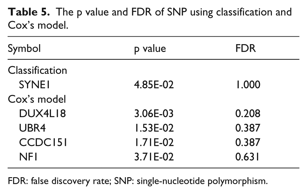
FDR: false discovery rate; SNP: single-nucleotide polymorphism.

Multivariate Cox’s model

Three significant clinical variables, 14 mRNAs, and two miRNAs were used to build the final integrated multivariate Cox’s model. After removing patients with any unavailable data, 304 patients’ data were used to train the model and 92 patients’ data were available for the testing dataset. The final model was as follows

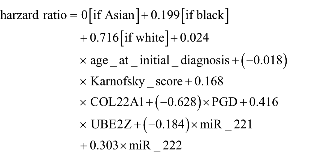
\begin{array}{l} harzard ratio = 0 [if Asian] + 0.199 [if black] \\ + 0.716 [if white] + 0.024 \\ \times age_at_initial_diagnosis + (- 0.018) \\ \times Karnofsky_score + 0.168 \\ \times COL 22 A 1 + (- 0.628) \times PGD + 0.416 \\ \times UBE 2 Z + (- 0.184) \times miR_221 \\ + 0.303 \times miR_222 \end{array}

The analysis of the hazard ratio was shown in Supplementary Figures 5 and 6. The log rank test and Kaplan–Meier plot were carried out on both the training and testing datasets (Figure 6). Eight signatures which were selected from all clinical features, mRNA expression level, and miRNA expression level performed well on both the training and testing datasets. The separation of low-risk and high-risk groups suggested that this model might be utilized in practice.

Figure 6.

The Kaplan–Meier plot using optimal models on both training (left) and testing (right) datasets by multivariate Cox’s model.

Discussion

We have performed classification and survival modeling to figure out biomarkers for the survival time of GBM. Both methods are commonly used to study the prognosis, but this study found that survival modeling was more suitable for GBM, and probably for other cancers, than classification. For classification, surprisingly, there were no significant clinical variables, mRNAs, miRNAs, or SNPs identified. On the contrary, survival modeling found successful biomarkers, which was proved using the testing dataset. It suggested that survival modeling might be a better method for biomarkers selection than classification.

There are two shortcomings of classification. One is that classification required two or more groups. When patients were separated into different groups, some of the censored data had to be removed. For example, in this case, 112 censored data with follow-up time less than 1 year were excluded, which accounted for 18.8% of all available cases. Also, GBM had a poor prognosis, so there are much less censored data than other cancers like prostate cancer or breast cancer. Classification will lose even more cases in studies of these cancers.

Second shortcoming is that it is hard to determine cutoffs or criteria to classify patients. For example, Patnaik et al.⁶ separated patients into groups of patients with recurrence and patients without recurrence in a study of non–small cell lung cancer. But in their study, the median recurrence time of patients with recurrence was much less than the median follow-up time of other patients. However, it is not the case in this study. Another study about non–small cell lung cancer used groups of patients who survived more than 30 months or less than 25 months to find out a pool of potential miRNA biomarkers, which were trained and tested by survival modeling later.⁷ Sboner et al.⁸ used 10 year as the cutoff in a study of prostate cancer, but they failed in improving prediction of disease progression with mRNA biomarkers. Marko et al.⁹ studied survival of GBM patients by separating them into groups of living longer than 24 months or shorter than 9 months, which excluded many patients.

Due to the above two reasons, methods of classification in this study failed in finding the prognostic biomarkers. But different criteria to separate the patients may succeed. On the contrary, survival modeling using Cox’s model or other models, such as the accelerated failure time model,¹⁰ does not have such shortcomings. And it succeeded in obtaining potential signatures for predicting GBM prognosis, even though Cox’s model has its own weakness, including that it is hard to interpret the hazard ratio into real survival time.

This study identified a group of clinical features, mRNAs, and miRNAs as potential prognostic biomarkers for GBM patients, which performed successfully in the testing dataset. Some of the biomarkers revealed by this study accord to known mechanisms, but few studies used them as biomarkers.

Three clinical variables were identified to be significantly related to survival time. They are age at initial diagnosis, Karnofsky score, and race. Interestingly, except for race, other two significant variables were both used as prognostic factors in recursive partitioning analysis of GBM.¹¹ This model separated patients into III, IV, and V + VI classes, defined by age, performance status, extent of resection, and neurologic function.¹² Here, the performance status was measured by Karnofsky score. Race is another significant variable. Surprisingly, the white had a higher hazard ratio than the black, and the Asian had the lowest hazard ratio. Multiple studies about GBM reported that there were no significant differences from the white and the black, but the Asian had a long survival time.^13,14 The former studies supported that the significant features could be used in the prediction of prognosis in GBM.

Although both selected mRNAs and miRNAs succeeded in predicting prognosis, most of these mRNAs were never reported to be related to any cancer, and none of these mRNAs were bound by miR-221 or miR-222. However, both miR-221 and miR-222 are oncogenic miRNAs.

When the biological functions of mRNA signatures were studied, it was quite interesting that genes encoding some of these mRNAs were related to inflammation. CLEC5A was reported to regulate inflammatory reactions and also control neuroinflammation through DAP12.¹⁵ HPGD is the main enzyme of prostaglandin degradation, which is involved in inflammation, and leads to anti-inflammatory effects. Such results may suggest that inflammation is one cause of bad prognosis in patients with GBM. The unrelated biological functions of mRNAs implied one possibility that it happened that these mRNAs had a lower p value. When Cox’s model prediction with a single variable was carried out, only CLEC5A, IZUMO1, and RANBP17 had a significant p value on the testing group. It suggested that other mRNAs might be related to survival status by chance on the training group due to the high variety of patients with cancer and smaller sample number in the testing group. Furthermore, the huge difference from p values of the training group and the testing group (3.0E-11 vs 9.7E-3) implied the over-fitting on the training group.

On the contrary, the two miRNA signatures, miR-221 and miR-222, are oncogenic miRNAs as reported. Interestingly, the genes encoding miR-221 and miR-222 occupy adjacent sites on the same chromosome. Moreover, their expression levels appear to be co-regulated, and they also seem to have the same specificity for the target.¹⁶ For example, both miR-221 and miR-222 are important regulators of p27^Kip1, which is a tumor suppressor and a cell cycle inhibitor. The higher activity and higher levels of miR-221 and miR-222 correlated with lower level of p27^Kip1 protein.¹⁶ It was also reported that miR-221 and miR-222 promoted the aggressive growth of GBM through suppressing p27^Kip1.^16,17 These studies supported that miR-221 and miR-222 might be potential prognostic biomarkers for GBM.

All in all, these eight signatures of clinical features, mRNA levels, and miRNA levels with significant p values on both the testing group and the training group need to be tested further on independent studies.

To conclude, this article used two different methods, classification and survival modeling, to figure out prognostic biomarkers for GBM. Although the classification method failed, signatures of clinical features, mRNA expression levels, and miRNA expression levels were figured out using Cox’s model. A multivariate model integrating all these information was built on the training dataset and validated on the testing dataset. It was proved to be a successful model, which has the potential to be used in clinics for personalized therapy for GBM patients.

Footnotes

Acknowledgements

Z.A. and L.L. are co-first authors.

Declaration of conflicting interests

The author(s) declared no potential conflicts of interest with respect to the research, authorship, and/or publication of this article.

Funding

The author(s) received no financial support for the research, authorship, and/or publication of this article.

References

Louis

Ohgaki

Wiestler

. The 2007 WHO classification of tumours of the central nervous system. Acta Neuropathol 2007; 114: 97–109.

Parsons

Jones

Zhang

. An integrated genomic analysis of human glioblastoma multiforme. Science 2008; 321: 1807–1812.

Ritchie

Phipson

. Limma powers differential expression analyses for RNA-sequencing and microarray studies. Nucleic Acids Res 2015; 43: e47.

Andersen

Gill

RD.

Cox’s regression model for counting processes: a large sample study. Ann Stat 1982; 10: 1100–1120.

Gandrud

SimPH: an R package for showing estimates for interactive and nonlinear effects from Cox proportional hazard models. J Stat Softw 2013, https://www.jstatsoft.org/article/view/v065i03

Patnaik

Kannisto

Knudsen

. Evaluation of microRNA expression profiles that may predict recurrence of localized stage I non-small cell lung cancer after surgical resection. Cancer Res 2010; 70: 36–45.

Chen

Zhao

. Serum microRNA signatures identified in a genome-wide serum microRNA expression profiling predict survival of non-small-cell lung cancer. J Clin Oncol 2010; 28: 1721–1726.

Sboner

Demichelis

Calza

. Molecular sampling of prostate cancer: a dilemma for predicting disease progression. BMC Med Genomics 2010; 3: 8.

Marko

Toms

Barnett

. Genomic expression patterns distinguish long-term from short-term glioblastoma survivors: a preliminary feasibility study. Genomics 2008; 91: 395–406.

10.

Wei

LJ.

The accelerated failure time model: a useful alternative to the Cox regression model in survival analysis. Stat Med 1992; 11: 1871–1879.

11.

Lamborn

Chang

Prados

MD.

Prognostic factors for survival of patients with glioblastoma: recursive partitioning analysis. Neuro Oncol 2004; 6: 227–235.

12.

Shaw

Seiferheld

Scott

. Reexamining the radiation therapy oncology group (RTOG) recursive partitioning analysis (RPA) for glioblastoma multiforme (GBM) patients. Int J Radiat Oncol Biol Phys 2003; 57: S135–S136.

13.

Barnholtz-Sloan

Maldonado

Williams

. Racial/ethnic differences in survival among elderly patients with a primary glioblastoma. J Neurooncol 2007; 85: 171–180.

14.

Thumma

Fairbanks

Lamoreaux

. Effect of pretreatment clinical factors on overall survival in glioblastoma multiforme: a Surveillance Epidemiology and End Results (SEER) population analysis. World J Surg Oncol 2012; 10: 75.

15.