Sage Journals: Discover world-class research

Abstract

Comparisons of survival times between screen-detected and symptomatically detected breast cancer cases are subject to lead time and length biases. Whilst the existence of these biases is well known, correction procedures for these are not always clear, as are not the interpretation of these biases. In this paper we derive, based on a recently developed continuous tumour growth model, conditional lead time distributions, using information on each individual's tumour size, screening history and percent mammographic density. We show how these distributions can be used to obtain an individual-based (conditional) procedure for correcting survival comparisons. In stratified analyses, our correction procedure works markedly better than a previously used unconditional lead time correction, based on multi-state Markov modelling. In a study of postmenopausal invasive breast cancer patients, we estimate that, in large (>12 mm) tumours, the multi-state Markov model correction over-corrects five-year survival by 2–3 percentage points. The traditional view of length bias is that tumours being present in a woman's breast for a long time, due to being slow-growing, have a greater chance of being screen-detected. This gives a survival advantage for screening cases which is not due to the earlier detection by screening. We use simulated data to share the new insight that, not only the tumour growth rate but also the symptomatic tumour size will affect the sampling procedure, and thus be a part of the length bias through any link between tumour size and survival. We explain how this has a bearing on how observable breast cancer-specific survival curves should be interpreted. We also propose an approach for correcting survival comparisons for the length bias.

Keywords

Lead time length bias breast cancer screening effect counterfactual survival

1 Introduction

Estimates for the mortality reduction due to screening based on observational studies are prone to biases, especially the so-called lead time bias and length bias, but also overdiagnosis.¹ Lead time is the difference in time from when the tumour would have been detected by symptoms, in the absence of a screening programme, to when the detection occurred in the presence of a screening programme. For screen-detected cases, this time will vary and may be a month or several years. Statistical analysis comparing survival times in populations with and without screening, or comparing screening to symptomatic cases in a population to which screening is offered, will be subject to lead time bias if survival is estimated as the time from diagnosis to death in screen-detected cancer. Any survival comparison, made to assess screening efficacy, should ideally be made from the time point at which symptomatic detection would have occurred.

The so-called length bias is a type of selection bias, which arises from screening cases over-representing tumours that, in the absence of screening, would be in a woman's body over a long time period before being detectable by symptoms. A length bias will result if survival time is associated with the time a tumour is present in the body before being detected.

If a woman's lead time exceeds the time from diagnosis until death, she is said to be overdiagnosed. Overdiagnosed women will introduce negative times to censoring (or deaths from other causes). It can be argued that such individuals should be excluded from survival comparisons. It is, in any case, important to report levels of overdiagnosis together with any such comparisons of survival, e.g. between screening and symptomatic cases.

There have been attempts to draw conclusions about screening efficacy using observational, cancer survival, data, and applying a variety of methods for correcting/diminishing lead time and length biases.^2–4 In the cancer screening research community, there is widespread awareness of the existence of lead time bias, length bias and overdiagnosis.^5–7 However, there is a need for further development of methods for bias correction and frameworks within which to assess screening efficacy from observational data.

Multi-state Markov models have long been the main modelling framework in the breast cancer screening literature to assess mammography screening sensitivity and sojourn time.^8–14 Although lead times have been estimated based on other approaches, using Bayesian methodology,^15,16 model-based studies of lead time, length bias and overdiagnosis have predominantly used multi-state Markov models with exponentially distributed sojourn times.^7,12,17,18 The sojourn time represents the period during which a tumour is asymptomatic but screen-detectable. The most basic of these models assumes that tumours progress through three states: no detectable cancer, asymptomatic but screen-detectable cancer and symptomatic cancer. Although several multi-state Markov models have been developed to incorporate categories of tumour size, lymph node status or other characteristics, the inherent discrete nature of the models may limit their suitability for studying/understanding the complexities of lead time, length bias and overdiagnosis. In particular, for the length bias, problems arise in understanding its complex nature by using the multi-state modelling framework, because the model does not distinguish the process of tumour growth from the process of symptomatic detection – it frames tumour progression in terms of sojourn times. Use of the model can potentially lead to misinterpretation of results, e.g. regarding the relationship between tumour growth and cancer survival.

Biological tumour growth models have recently been proposed which break with, and represent a promising alternative to, multi-state models. For instance Atkinson et al.,¹⁹ Brown et al.²⁰ and Bartoszyński et al.²¹ proposed the use of a combined model for tumour growth and symptomatic tumour detectability, for data in absence of screening. Plevritis et al.²² extended this to further include, in addition to tumour size, also lymph nodal and distant metastases. Weedon-Fekjær et al.²³ presented a continuous tumour growth model combined with a continuous function of screening sensitivity (according to tumour size). These types of tumour growth models are likely to better represent the underlying biology of tumour growth than the multi-state Markov model. Weedon-Fekjær et al. showed that their model gave a better fit to incidence data (from a mammography screening cohort) than a multi-state Markov model and argued that the latter may underestimate the variability in growth rates. The approach of Weedon-Fekjær et al.^14,23 does, however, not model symptomatic detection. Abrahamsson and Humphreys²⁴ recently proposed a continuous tumour growth model for screening data which explicitly describes three continuous processes; tumour growth, time to symptomatic detection and screening sensitivity. In this paper, we describe approaches for quantifying lead time, and share new insights into length bias and studying effects on survival, based on their model.

2 A continuous tumour growth model

The first submodel proposed in Abrahamsson and Humphreys²⁴ is for tumour growth. It assumes that tumours are spherical and grow exponentially with a constant volume doubling time. For a tumour growing with an inverse growth rate r, t years after tumour onset, the volume, measured in cubic millimeters, is specified as

V (t, r) = V_{0} e^{t / r}, t \geq 0, r > 0

(1)

where V₀ is the tumour volume at which the earliest possible detection occurs (V₀ corresponds to a tumour diameter of 0.5 mm). To capture heterogeneity in growth rates, r is considered as a realisation from the random variable R, following a gamma distribution with shape and rate parameters τ₁ and τ₂. In addition to leading to mathematically tractable results in our context,²⁵ the exponential growth model has been shown by Talkington and Durrett²⁶ to give a better fit to breast cancer in-vivo data than Gompertz, logistic and power law growth models. Other researchers have, however, argued for these other growth models.²⁷

The second submodel describes the process by which tumours are detected by symptoms.²⁴ It assumes that the time from tumour onset to symptomatic detection, T_det, depends on the tumour volume through a hazard function

P (T_{\det} \in [t, t + dt) | T_{\det} > t, R = r) = η V (t, r) dt + o (dt), V (t, r) \geq V_{0}

(2)

The third submodel describes mammography screening sensitivity²⁴ using a logistic function of tumour diameter, d, in mm, and other characteristics, such as percentage mammographic density, m $(0 \leq m \leq 1)$ , for example

S (d, m) = \frac{exp (β_{1} + β_{2} d + β_{3} m)}{1 + exp (β_{1} + β_{2} d + β_{3} m)}

(3)

Mammographic density decribes the breast tissue composition seen on a mammogram. Fibro-glandular tissues have a high mammographic density and are seen as white, whilst fatty tissues that appear dark and have low mammographic density. Since tumours appear white on mammograms, they may be masked in breasts with a high amount of dense tissue.

Isheden and Humphreys²⁵ describe how the unknown parameter values of the three submodels can be estimated from breast cancer incident cases identified in a screened population by maximising a likelihood function, based on the conditional distribution of tumour size, given a woman's screening history, detection mode and percentage mammographic density.

3 Conditional lead time distributions

Based on the multi-state Markov model with exponentially distributed sojourn times, the mean lead time of screen-detected cases will be equal to the (population) mean sojourn time (due to the memoryless property of the exponential model). The most used lead time correction presented by Duffy and colleagues¹⁸ is based on the multi-state Markov model and subtracts this (estimated) mean sojourn time from survival times of screen-detected cases. Although there is reason to believe that this (unconditional) correction can work well in practice (see Section 4.4), it is not realistic to assume that (conditional) distributions of lead times are equal across tumours, e.g. if we condition on characteristics such as tumour size at screen detection, times since previous negative screens and mammographic density. Based on a similar model, conditional lead time distributions, taking screening history into account and using age-specific mammography screening sensitivity, have recently been presented by Lee et al.¹² Tumour size/stage was, however, not conditioned on. For our continuous growth model, it is possible to calculate well-defined lead time corrections on an individual level basis (Section 4.3). We show, first, how conditional lead time distributions can be calculated based on submodels (1) to (3).

3.1 Calculations of conditional lead time distributions

Let l be the lead time (i.e. time between detection in the presence of a screening programme and detection in the absence of a screening programme). Further, let l be a realisation from a random variable L. It is assumed that L = 0 for cases detected by symptoms and that L > 0 for cases detected by screening. In order to derive the (conditional) density function for L (given screening history, tumour size at detection and mammographic density), for screen-detected cases, we base our calculations on the assumption of a stable disease population (an assumption that is also present in the multi-state Markov models). That is, we assume that the distribution of age at tumour onset and the rate of births in the population are constant across calendar time. The covariate percentage mammographic density is for ease of exposition omitted in the following formulae, but is straightforward to include (and is included in analyses described in Section 3.2).

In what follows, we use results derived in Isheden and Humphreys²⁵ for the growth models (1) to (3) in a stable disease population, in the absence of screening. First, the conditional inverse tumour growth rate distribution, given a tumour of size C(s) (in an unscreened population at any calendar time point, s), follows a gamma distribution

f_{R | C (s) = c, A (s) = 1} (r) = \frac{τ_{2} + η (c - V_{0})}{Γ (τ_{1} + 1)} (r (τ_{2} + η (c - V_{0}))) τ_{1} e^{- r (τ_{2} + η (c - V_{0}))}

(4)

C(s) denotes tumour volume in cubic mm at calendar time point s, and A(s) is a dichotomous variable, equaling 1 if the tumour is present in the breast at time point s, and 0 otherwise. Second, in the absence of screening, the conditional distribution for symptomatic tumour size (measured in mm³), V_det, given C(s), and inverse tumour growth rate, R, has density

f_{V_{\det} | C (s) = c, A (s) = 1, R = r} (v) = η r e^{- η r (v - c)}

(5)

From equations (1) to (5), we show in Appendix 1 that, in the presence of screening (assuming that screening attendance is indepedent of growth rate)

\begin{matrix} f_{L | C (s) = c, A (s) = 1, B (s) = 1, B^{c}} (l) \propto \int_{0}^{\infty} f_{R | C (s) = c, A (s) = 1} (r) f_{L | C (s) = c, A (s) = 1, R = r} (l) P (B^{c} | R = r, C (s) = c, A (s) = 1) dr \end{matrix}

(6)

where

B^{c} = (B (s_{- k}), \dots, B (s_{- 1})) = (0, \dots, 0)

and B(s) is a dichotomous variable defined at the time points where a screening occasion was present, equaling 1 if the woman has a tumour detected by screening at time point s, and 0 otherwise. The calendar time point for the

k^{th}

last negative screening is expressed as

s_{- k}

and women with previous positive screens are not included. B^c thus explains all screening history, excluding any screening leading to diagnosis. The first term within the integral above is obtained from equation (4). The second term can be shown to be a Gompertz density. By using the exponential tumour growth assumption (1), which leads to

L = R log \frac{V_{\det}}{C (s)}

, it is possbile to derive the conditional distribution function for lead time given tumour size at screen detection and inverse tumour growth rate. By using

F_{L | C (s) = c, A (s) = 1, R = r} (l) = F_{V_{\det} | C (s) = c, A (s) = 1, R = r} (c e^{l / r})

(7)

together with equation (5), we arrive at

f_{L | C (s) = c, A (s) = 1, R = r} (l) = \frac{c}{r} e^{l / r} f_{V_{\det} | C (s) = c, A (s) = 1, R = r} (c e^{l / r}) = η c e^{- η rc exp (l / r) + η rc + l / r}

(8)

The third term within the integral (6) can be read as “the probability for not being detected at previous negative screens at time points $s_{- k}, \dots,, s_{- 1}$ , given tumour growth rate and tumour size at time point s”. We let $c_{- k}$ be the corresponding tumour volume at time point $s_{- k}$ , and further use the assumption of exponential tumour growth to write $c_{- k} = \frac{c}{exp (\frac{s - s_{- k}}{r})}$ . By using the sensitivity function (3) and transforming the volume to diameter (under the assumption of tumours being spherical), it can be shown that for a woman with k negative screens

P (B^{c} | R = r, C (s) = c, A (s) = 1) = (1 + e^{β_{0} + β_{1} {(\frac{6}{π} c_{- 1})}^{1 / 3}})^{- 1} \cdot \dots \cdot (1 + e^{β_{0} + β_{1} {(\frac{6}{π} c_{- k})}^{1 / 3}})^{- 1}

(9)

3.2 Heterogeneity of lead time distributions in breast cancer

Using the results in Section 3.1, we now demonstrate the heterogeneous nature of (conditional) lead times; in Figure 1 we have plotted individual (conditional) lead time distributions based on different tumour sizes at diagnosis, screening histories and percentage mammographic densities. These calculations are based on parameter values τ₁ = 2.36, τ₂ = 3.00, η = e^−8.75, β₁ = –4.75, β₂ = 0.56 and β₃ = –1.95. The growth rate parameter τ₁ and the mammography screening sensitivity parameters β₁, β₂ and β₃ were taken directly from Abrahamsson and Humphreys,²⁴ from an analysis applying our model to a sample of Swedish incident invasive breast cancer cases (from the same study base as the data presented in Section 4.1) and fitting to tumour size distributions of symptomatic and screen-detected cancers separately. The value of the other growth rate parameter τ₂ was adapted to ensure that the growth rate distribution is roughly in line with the growth rate distribution estimated in Weedon-Fekjær et al.,¹⁴ using a large Norwegian mammography screening cohort and fitting a model to both tumour size (screen-detected cases) and interval cancer (a term used in the screening literature to describe cases detected symptomatically between screening rounds in women regularly attending screening) incidence data. The value of η, for the model of symptomatic detection (that would result in the absence of screening), was estimated based on the same type of analysis as described above for τ₁, β₁, β₂ and β₃ using the data described in Section 4.1, but conditioning on the adapted growth rate parameter τ₂. We note that in our simulation study, described in Section 4.2, our final choice of parameter values resulted in median tumour diameters of 12 mm and 19 mm, for screen-detected and interval cancers, respectively, when imposing a biannual screening programme between the ages of 40 and 74 (see Section 4.2), which were the same median tumour sizes as were observed in our real data analysis (Section 4.1). Also in the simulated data, the chosen parameter values lead to similar proportions of screen-detected and interval cancers among screen-attenders (70% vs. 30%) as presented in Törnberg et al.²⁸

Figure 1.

Individual lead time distributions for screen-detected cases based on tumour size, screening history and percentage mammographic density.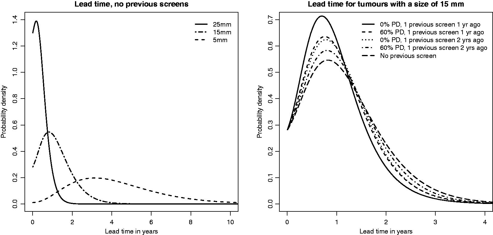

The (inverse) growth rate distribution corresponds to a distribution of times for a tumour to grow from 10 mm to 15 mm in diameter having 5th, 25th, 50th, 75th and 95th percentiles of 2.4, 6.0, 9.9, 15.3 and 25.8 months. The parameters of the mammography screening sensitivity model correspond to sensitivities of 0.06, 0.36, 0.84 and 0.98 at 4 mm, 8 mm, 12 mm, 16 mm and 20 mm, respectively in breasts with 15% mammographic density. The parameter of the symptomatic detection model corresponds to a (cumulative) probability of a tumour being (symptomatically) detected by the time it reaches 12 mm, in the absence of screening, of 0.39 (averaged over the inverse growth rate distribution).

From Figure 1 it is clear that the tumour size at screen detection plays the major role for the lead time distribution. A tumour detected at a small tumour size is much more likely to have a long lead time than a tumour detected at a large tumour size. The lead time distribution is, however, flattest for tumours that are small at diagnosis, meaning that it is difficult to know whether small tumours have been existing for a longer time or have started to grow only recently. Further, lead times increase with percentage density. Growth rates will, on average, be slower for masked tumours than for unmasked tumours. This effect of mammographic density is, however, small in comparison to the effect of tumour size. We note that the differences in lead time across groups of women having high and low values of percentage mammographic density would be much more different if tumour size had not been conditioned on. Not surprisingly, lead times were slightly shorter for women with previous negative screens, especially when the screens were close in time to the diagnostic screening.

Based on Figure 1 it is evident that estimated lead times used in this article are shorter than in the paper describing the average (unconditional) lead time correction based on the three state Markov model (Duffy et al.¹⁸), where a mean value of four years was assumed. This is, to some extent, because the continuous growth model does not support the memoryless property (which forces lead times to follow the same distribution as sojourn times) – see also Section 4.5. The estimated lead times are, however, in closer agreement with the values presented by Chen et al.¹⁵

4 Lead time bias corrections and length bias – a simulation study and an illustrative example using Swedish (invasive) breast cancer data

Derived conditional lead time distributions can be used for making a lead time bias correction when comparing survival times of screening cases to symptomatic cases, or comparing survival times of cases collected in the presence of a screening programme to cases collected in the absence of a screening programme (ensuring that time is measured from comparable time points for all cases). There are, however, different ways of using the distributions. In this paper we suggest an approach based on sampling one or a few lead times for each woman from her specific (conditional) lead time distribution (Section 4.3). We use simulated data (Section 4.2) and data on Swedish postmenopausal invasive breast cancer patients (described in Section 4.1 to present our approach and to compare it to the average method (see Sections 4.4-4.5). We also use simulated data to make some further points concerning length bias (Section 4.6). In the simulation, the same set of women are being followed under two different counterfactual scenarios of screening. Thomas²⁹ also used several counterfactual screening scenarios in order to study biases arising in different estimates of the screening effect for colorectal cancer.

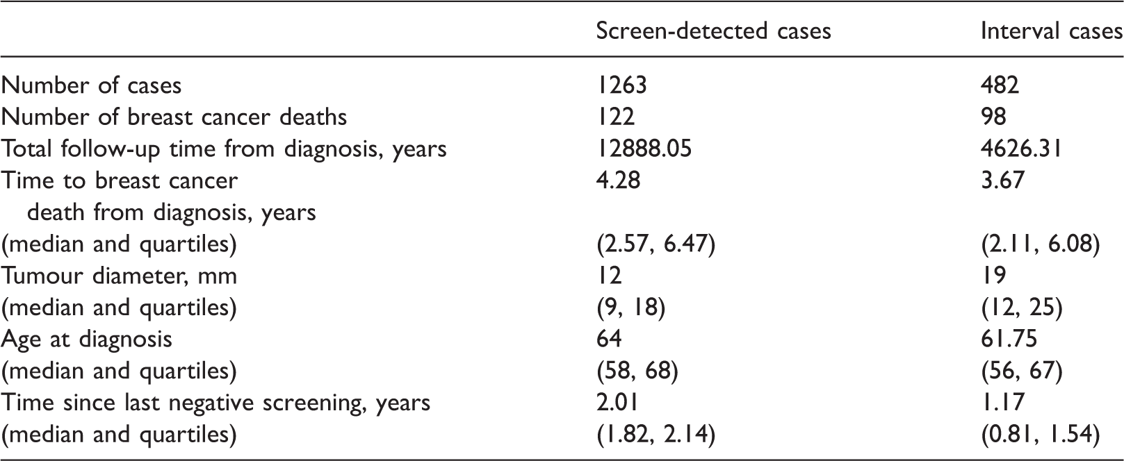
4.1 Swedish postmenopausal breast cancer data

We make use of data collected on 1745 postmenopausal women, attending the Swedish national screening programme, who were diagnosed with incident primary invasive breast cancer in Sweden between October 1993 and March 1995. These women were included in CAHRES, a case-control study of women between 50 and 74 years old at diagnosis, which had a participation rate of 84% among the 3979 eligible cases found through Swedish Cancer Registries. The data collection has been described elsewhere.^30–33 The 1745 postmenopausal patients used here all had information on detection mode (screening vs. interval), screening history, tumour size at diagnosis and had follow-up information on deaths due to breast cancer or other causes (from the Swedish cause of death register and the Swedish migration register) up until 31 December 2015. Interval cases were defined as women diagnosed with a symptomatic cancer within two years from a negative screening round. Other symptomatic cases in non-regular screen-attenders were excluded (n = 377) as the focus of this paper is not to study any possible healthy-volunteer bias. Of the 1745 women included in our study, 28% were interval cancers and 72% were screen-detected cases. See Table 1 for a descriptive comparison of the screen-detected and interval cases.

Table 1.

Descriptive comparison of screen-detected and interval cases in CAHRES.

	Screen-detected cases	Interval cases
Number of cases	1263	482
Number of breast cancer deaths	122	98
Total follow-up time from diagnosis, years	12888.05	4626.31
Time to breast cancer death from diagnosis, years	4.28	3.67
(median and quartiles)	(2.57, 6.47)	(2.11, 6.08)
Tumour diameter, mm	12	19
(median and quartiles)	(9, 18)	(12, 25)
Age at diagnosis	64	61.75
(median and quartiles)	(58, 68)	(56, 67)
Time since last negative screening, years	2.01	1.17
(median and quartiles)	(1.82, 2.14)	(0.81, 1.54)

Ethical approval was obtained from the Regional Ethics Review Boards in Uppsala at Uppsala University and in Stockholm at Karolinska Institutet. Written informed consent was provided from all participants.

4.2 Data simulation procedure

To demonstrate our lead time bias correction and to compare it to the average method based on multi-state Markov modelling, as well as to explain additional points about the length bias, we carried out a simulation study. We generated (in-silico) individuals as being born into a cohort uniformly at a rate of 160,000 births per year. These individuals were followed under two different circumstances, in the presence and absence of a screening programme. The simulation was run for a length of time sufficient to achieve burn-in (see below), after which, over a two-year period, incident breast cancer cases were selected. Data from these (approximately 34,000) cancer cases of screening age were then analysed.

We generated individuals, continuously over time, from a stable disease population. That is we simulated individuals being born into a cohort at a constant rate, over a long time period to ensure that the incidence of cancer was constant over time. Age-specific breast cancer incidence rates from The Swedish National Board of Health and Welfare (according to rates from 2016),³⁴ subsequently shifted with five years towards lower ages, were used to generate an age at tumour onset, in a similar manner to Forastero et al.³⁵ The value of 5 years was close to the mean value of time between tumour onset and detection as seen in the simulation. For each individual with cancer, we simulated death from breast cancer both in the absence and presence of screening (described below). For all individuals we simulated a time of death from other causes, according to Swedish age-specific mortality rates (values of 2016) from Statistics Sweden.³⁶ For individuals getting breast cancer with an age at onset before the generated age of death from other causes, tumours were assumed to be spherical and to have an onset diameter of 1 mm. Data were simulated under the continuous growth model functions (1) and (2). For each woman, independent of tumour onset time point, an inverse tumour growth rate was sampled from a gamma distribution with shape parameter, $τ_{1} = 2.36$ , and rate parameter, $τ_{2} = 3.00$ (the choice of parameter values was described in Section 3.2). Conditional on the values of these parameters, each woman was assigned a specific tumour size (in mm³) at symptomatic detection, sampled from the conditional distribution of symptomatic tumour sizes given inverse growth rate (see formula (5) in Abrahamsson and Humphreys²⁴) using $η = e^{- 8.75}$ in the hazard function (2).

In the presence of screening, biannual screening between the ages of 40 and 74 was superimposed and at each screen, screening sensitivity was calculated using the logistic function (3), with parameters $β_{1} = - 4.75, β_{2} = 0.56$ and $β_{3} = - 1.95$ . For simplification purposes, percentage mammographic density was assumed to be 15%, close to the median value presented in Isheden and Humphreys²⁵ and screen attendance was assumed to be complete. Tumour sizes at screening were inferred from the onset times and inverse growth rates. The lead time for each screen-detected cancer was calculated by subtracting the time point for detection in the presence of screening from the time point for detection in the absence of screening. Thus, lead times were all equal to or larger than zero. Before selecting data for our analyses we waited for an amount of time (120 years), which was sufficient to ensure burn-in, in terms of e.g. a constant mortality rate, and then select all incident cancers within a study period of 2 years. Approximately 30% of cancers are detected as interval cancers and 70% are screen-detected.

In both the presence and absence of screening, death was either from breast cancer or other causes, whichever occurred first. One of the main points we make in this article is about the impact of a possible relationship between growth rate and survival. Due to limitations in existing modelling approaches, this relationship has never been quantified. We could therefore only explore different combinations of parameter values in order to obtain values of the model which corresponded to results from observational studies on tumour size distributions and the relative proportions of screen/interval detected cancers. When fitting a Weibull distribution to our observational data (Section 4.1), the shape parameter value was estimated to be close to 1 (corresponding to an exponential distribution). Because of this and the fact that it is easier to search the parameter space of an exponential, than a Weibull distribution, we searched the parameter space of exponential models which incorporated effect of tumour growth on survival, in order to choose parameter values of the survival time models which were consistent with survival time distributions that were similar to those in our observational data, for interval and screen-detected cancers. To ensure no woman dies before her lead time has passed, all women were at risk of dying from breast cancer from the time at which they would have been symptomatically detected.

For each woman we recorded the survival time in the absence, S_abs, and the presence, S_pres, of screening, which are assumed to follow exponential distributions

S_{abs} \sim exp (λ \cdot d_{abs} + γ / r), S_{pres} \sim exp (λ \cdot d_{pres} + γ / r)

(10)

where r is the inverse tumour growth rate and d_abs and d_pres are the tumour diameters in mm at detection, in, respectively, the absence, and the presence, of screening. Note that, in the presence of screening, survival S_pres is measured from the time point of symptomatic detection, whilst d_pres is the tumour size occurring at the time point of a possible screen detection. This, in addition to our assumption of exponential survival times, is clearly a simplification, and is perhaps not what we would expect from real data. The simulation, however, serves perfectly well for the purpose of demonstrating lead time and length biases. Parameter values λ = 6⋅10⁻⁴ and γ = 4⋅10⁻³ were used. See Table 2 for an example of predicted 10-year breast cancer specific survival rates in absence of screening, for different values of tumour size at diagnosis and inverse tumour growth rate. For an example with tumour growth rate not affecting survival, λ = 1.2⋅10⁻³ and γ = 0 were used. Both sets of parameter values, when used in our simulation study, in combination with the other models, corresponded to results from observational studies on tumour size distributions and the relative proportions of screen/interval detected cancers and survival time distributions of screen vs. interval cancers (on both an aggregated level and stratified on tumour size).

Figure 2.

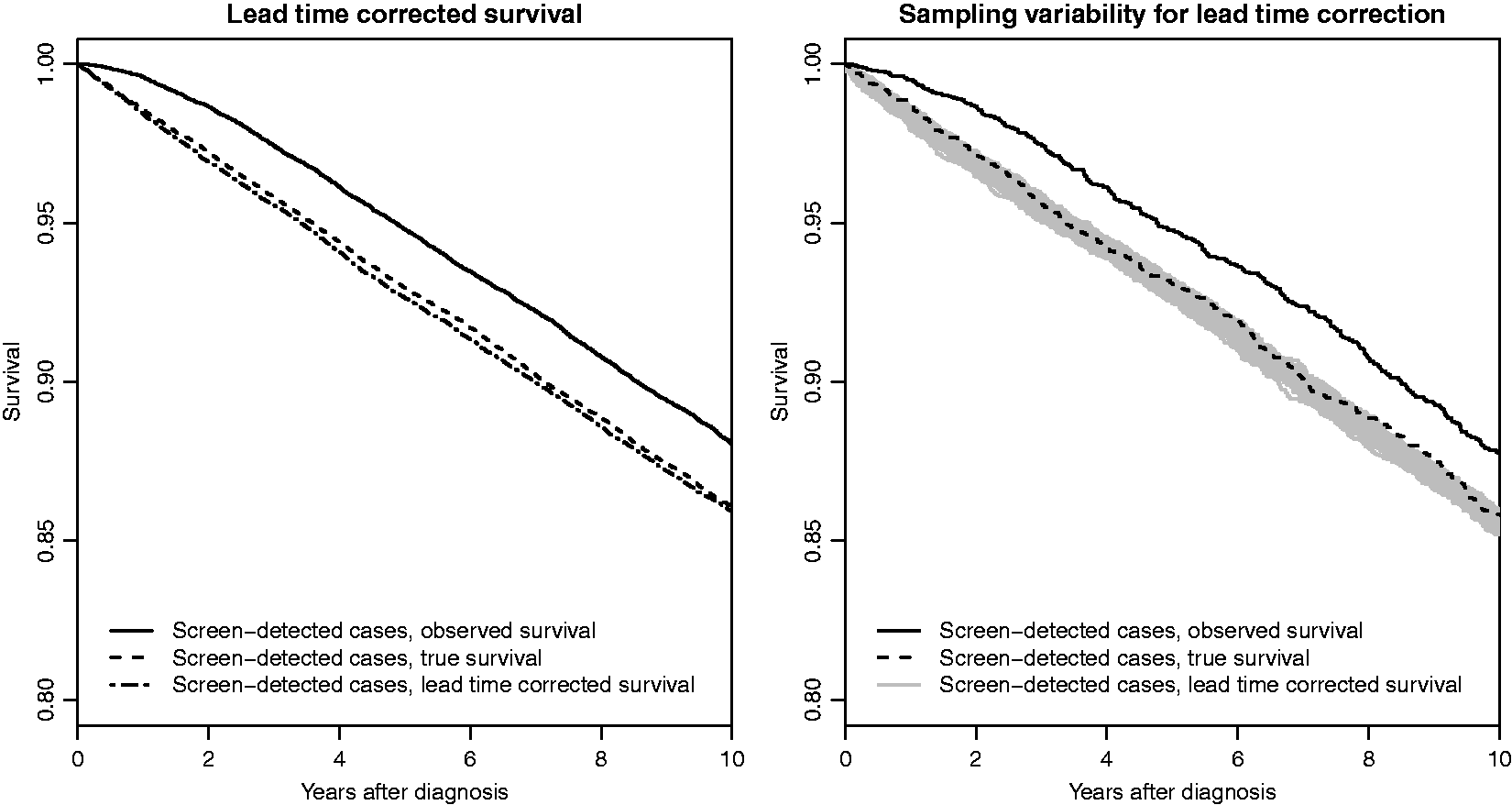
Lead time corrected survival based on the individual correction, for simulated data.

Table 2.

Predicted 10-year breast cancer specific survival rates in absence of screening, for different values of tumour size at diagnosis and inverse tumour growth rate, using parameter values λ = 6⋅10⁻⁴ and γ = 4⋅10⁻³ in the time to death function (10).

	Inverse tumour growth rate
Tumour size	0.25	0.75	1.25
10 mm	80.2%	89.5%	91.2%
20 mm	75.7%	84.1%	85.8%
30 mm	71.2%	79.2%	80.9%

In the simulation, we imposed both a lead time bias (by making sure that no woman can die before her lead time has passed) and a length bias (by allowing the tumour growth rate to affect the survival time). We also simulated a true screening effect by making the survival dependent on tumour size. We note that, following this simulation procedure, we could estimate overdiagnosis, e.g. as the percentage of screen-detected cancers that would not have been detected within the women's lifetimes, in the absence of screening. Since our parameter values are based on invasive breast cancer data, the level of overdiagnosis was very low (approximately 2%).

4.3 A lead time correction based on conditional lead time distributions

For our lead time correction, we sample from conditional lead time distributions, and for each woman we subtract a sampled lead time, $l^{*}$ , from the observed (breast cancer) survival time, s_obs. This simple adjustment is similar to that suggested by Duffy et al.¹⁸ in the context of the multi-state Markov model. If we let d_t represent the calendar time point for breast cancer death (for women with non-censored survival times) and s represent the calendar time point for screen detection, then $L \leq d_{t} - s$ must hold. Hence, the lead time will follow the truncated conditional distribution

\begin{matrix} f_{L | C (s) = c, A (s) = 1, B (s) = 1, B^{c}, L \leq d_{t} - s} (l) = \frac{f_{L | C (s) = c, A (s) = 1, B (s) = 1, B^{c}} (l)}{F_{L | C (s) = c, A (s) = 1, B (s) = 1, B^{c}} (d_{t} - s)}, 0 \leq l \leq d_{t} - s \\ = 0, otherwise \end{matrix}

(11)

For women with survival times that are censored due to end of, or loss to, follow-up, we proceed as follows. We first sample from $f_{L | C (s) = c, A (s) = 1, B (s) = 1, B^{c}} (l)$ . If g_t denotes calendar time point of censoring and the sampled lead time value exceeds $g_{t} - s$ , the woman is excluded from the survival analysis since she will have a negative (and censored) survival time (with respect to the sampled symptomatic detection). This exclusion also ensures that we are comparing like with like, i.e. as if we had sampled both screening and symptomatic cases according to their symptomatic detection dates.

To simplify, deaths from causes other than breast cancer can also be treated as censored events. We would suggest using exactly the same procedure as above. Excluding women from the survival analysis, when $L > g_{t} - s$ , represents, in this case, the exclusion of overdiagnosed women. If g_t is the time point for censoring, not due to death from other causes, but due e.g. to loss to follow-up, it is, of course, not possible to know whether the woman was overdiagnosed.

Sampling from the conditional density function (6) is possible, but time-consuming in practice, since one numerical integration for each screening case needs to be performed. We instead use a procedure which gives equivalent results but is much faster. Instead of sampling directly from $f_{L | C (s) = c, A (s) = 1, B (s) = 1, B^{c}} (l)$ , we first sample an inverse growth rate, $r^{*}$ , from

f_{R | C (s) = c, A (s) = 1, B (s) = 1, B^{c}} (r)

(12)

which can be obtained in closed-form (see Appendix 2), and subsequently sample a lead time,

l^{*}

, from the conditional density function

f_{L | C (s) = c, A (s) = 1, B (s) = 1, B^{c}, R = r^{*}} (l)

, which can equivalently be sampled from

f_{L | C (s) = c, A (s) = 1, R = r^{*}} (l)

using equation (8). This simplification can be made since screening history and screening outcome do not contribute additional information about lead time, once inverse tumour growth rate is known. For women with the end point death by breast cancer, in the case that

l^{*} > d_{t} - s

, the procedure is repeated (until

l^{*} \leq d_{t} - s

) – this is equivalent to sampling from the truncated distribution (11), directly. As discussed above, for censored cases, if

l^{*} > g_{t} - s

, then that case is excluded from the survival analysis.

For each screen-detected woman, the sampled lead time value is subtracted from the observed survival time, s_obs, to obtain a lead time corrected survival, $s_{pres}^{*}$

s_{pres}^{*} = s_{obs} - l^{*}

(13)

which is measured from the time at which the symptomatic detection would have occurred. If we use this procedure to compare survival times before and after the introduction of a screening programme, we implicitly assume that symptomatic detection occurs at the same time point before and after introduction of the programme. The validity of such an assumption could be questioned (there may be an increase in breast cancer awareness among women following the introduction of a screening programme, alternatively women do not seek health care immediately when feeling symptoms but awaits their next screen examination). This will be less of an issue for making comparisons between screen and symptomatically detected cancers collected at the same time (in a population to which screening is offered).

To show that our lead time bias correction works, we compare the ‘true’ survival times in the presence of a screening programme, s_pres, (measured from when symptomatic detection would have occurred) to lead time corrected survival times, $s_{pres}^{*}$ . We use parameter values λ = 6⋅10⁻⁴ and γ = 4⋅10⁻³ in equation (10). At this point, we include only screening cases so that there is no length bias (here, we are not comparing non-exchangeable groups, such as screening to interval cases). For the simulated data, which has approximately 24,000 screen-detected breast cancer cases, the survival times are plotted as Kaplan–Meier curves, in Figure 2 (left side). The solid line represents observed survival, s_obs, measured from screen diagnosis. The lead time corrected survival, $s_{pres}^{*}$ , (line with dots and dashes) is close to the true survival, s_pres, (dashed line) for these screen-detected cancers – the corrected is seen to provide an unbiased survival estimate. To examine sampling variability we sampled 100 sets of lead times, one per woman, for a sample of 3000 screen-detected cases. Results are presented in Figure 2 (right side). The grey region represents 100% coverage.

Figure 3.

Comparisons of individual and average lead time corrections for simulated screen-detected cases; 50% smallest tumours to the left and 50% largest tumours to the right. The median tumour size was 12 mm.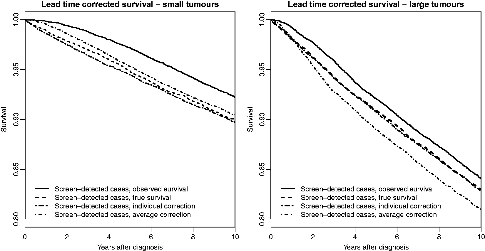

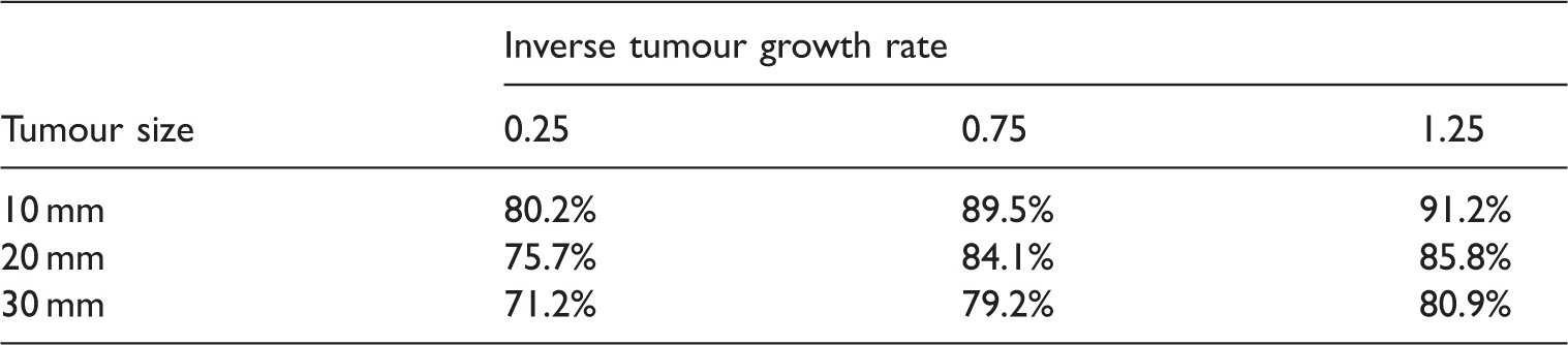
4.4 Comparing individual and average lead time corrections using simulated data

To use the average correction on the simulated data set, we need an estimate of the transition rate from the asymptomatic but screen-detectable state to the symptomatic state. We obtained an estimate using the R-script for fitting a multi-state Markov model, presented in Weedon-Fekjær et al.,¹⁴ which incorporates conditioning on screening history. We estimated the yearly transition rate to be 0.48 (1/mean sojourn time) using our simulated data. 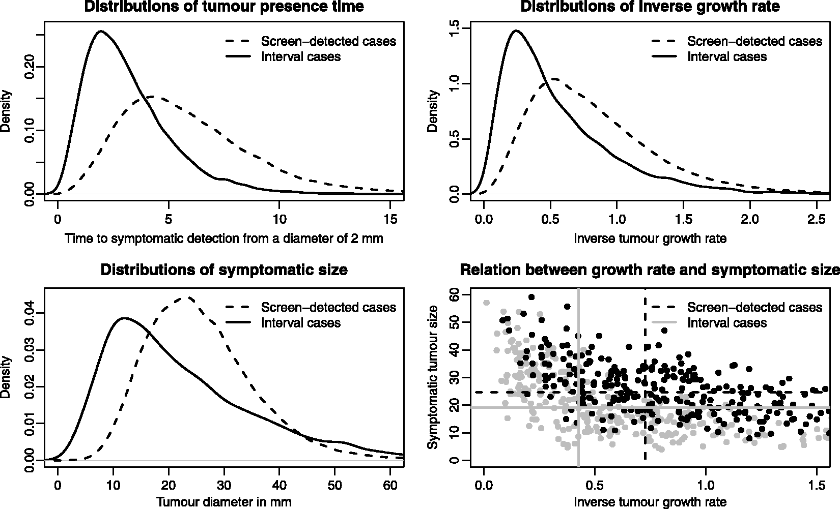This estimate was used in the lead time correction procedure described by Duffy et al.¹⁸ to obtain an average lead time corrected survival, ${s_{pres}}^{^}$ . Despite the differences in the underlying model assumptions, in an overall analysis, the correction works well (data not shown; the corrected survival curve is slightly below, but close to, the true survival – although the data is simulated using the continuous growth model). However, when the correction is used within strata, it works less well, if the variable being stratified on is correlated to the lead time. We exemplify this by correcting survival using both methods (individual and average lead time corrections) in analyses stratified on tumour size (strata defined according to being below/above the median tumour size at diagnosis, being 12 mm among screen-detected cases in both the simulated data and in the CAHRES data), based on simulated data (Figure 3) and the 1263 screen-detected breast cancers described in Section 4.1 (Figure 4). For the individual lead time correction applied to the CAHRES-data, 10 conditional lead time values were sampled for each woman to reduce variability. The interval cases (not shown in the figure) had seven-year survival rates of 97% for tumours smaller than or equal to 12 mm and 77% for tumours larger than 12 mm. Overall, the corrections for small tumours look similar, but for large tumours the average method clearly over-corrects. In general we can conclude that, using an average method (based on unconditional lead time distributions) will lead to an over-correction for tumours having short lead times and an under-correction for tumours having long lead times. This issue is likely to have arisen in the survival comparison presented in Allgood et al.³ where they study differences between lead time corrected survival times in screening cases and survival times in symptomatic cases, stratifying on tumour size and nodal involvement.

Figure 4.

Comparisons of individual and average lead time corrections for Swedish postmenopausal screen-detected cases; 50% smallest tumours to the left and 50% largest tumours to the right. The median tumour size was 12 mm.

Figure 5.

Distributions (as if screening was not present) of tumour presence time, inverse growth rate and symptomatic size (and marginal medians for the two last quantities) from simulated data, by detection mode (screening/interval), in the presence of screening. Based on parameter values τ₁ = 2.36, τ₂ = 3.00 (inverse tumour growth rate distribution) and η = e^−8.75 (hazard rate for symptomatic detection).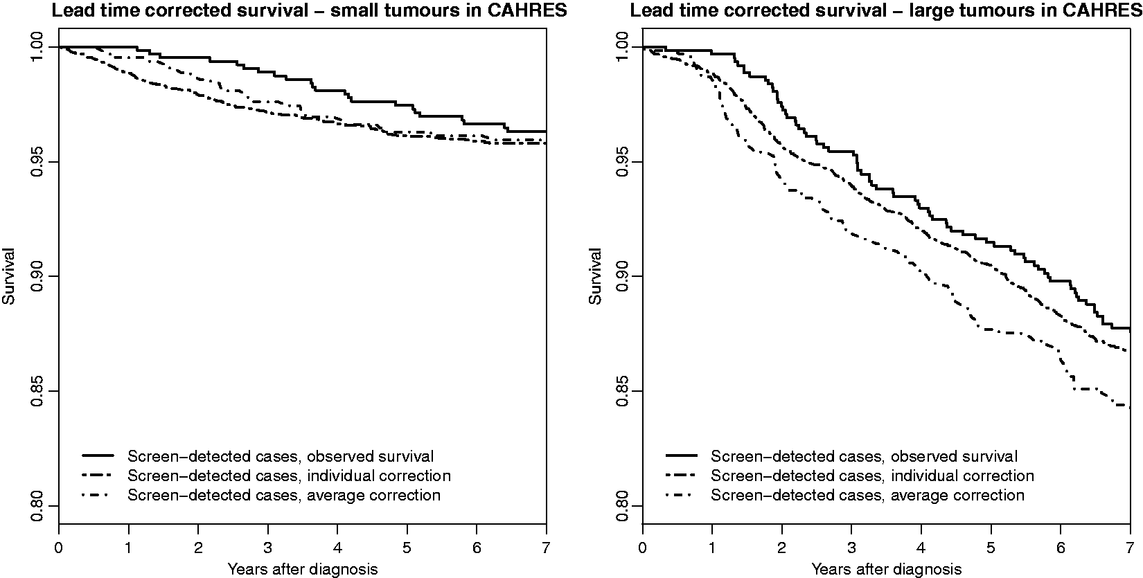

4.5 Effect of the memoryless assumption in multi-state Markov models on lead times

For our continuous growth model, we cannot define a quantity that is equivalent to that of the multi-state Markov model's sojourn time. We can, however, define a ‘tumour presence time’, as the time from when the tumour is of a specific size until symptomatic detection. Using a starting diameter of 2 mm, in the simulated data set, the mean tumour presence time in the absence of screening was 5.06 years with a 95% confidence interval of (5.02, 5.09), whilst the mean lead time was 1.94 years with a 95% confidence interval of (1.92, 1.97) (for the screening cases). Based on the simulated data, to obtain a mean tumour presence time which is the same as the mean lead time, we would need to start measuring time from when the tumour was 8 mm, which is clearly long after the time point tumours become screen-detectable (22% of the screening cases in the simulation were smaller than 8 mm at diagnosis and tumours started to be detectable at around 2 mm). The memoryless assumption, however, only partly explains the differences in mean lead times, from 1.94 years to the approximately four years that is assumed in Duffy et al.¹⁸ The mean sojourn time estimated in our simulated data set (using the procedure explained in the previous section) was 2.09 years with a 95% confidence interval of (2.07, 2.12). The confidence intervals were obtained by estimating or calculating averages of the quantities, based on 100 large simulated data sets (with approximately 34,000 cases each).

4.6 A novel view on length bias

A woman with a long tumour presence time has an increased chance of being screen-detected. This phenomenon is called length-biased sampling and is of interest because it will lead to biased survival comparisons (between e.g. screening and interval cases) if tumour presence time affects not only the sampling, but also survival time per se.

The traditional view of length bias is that screening cases may have better survival than interval cases (after lead time adjustment) partly due to differences in tumour growth rates. The biomarker Ki-67, which is expressed by proliferating cells and likely to be correlated with growth rates has, for example, been shown in a meta-analysis to be an independent prognosticator in early breast cancer.³⁷ The above view of length bias originates from the application of the multi-state Markov model to cancer screening data. It is easy to fall into the trap of considering the rate of transition from asymptomatic to symptomatic cancer to be driven solely by the rate of tumour growth/progression, when, in fact, the transition rate is an overall effect of both tumour growth rate and time to symptomatic detection. The wide range of tumour sizes at diagnosis among symptomatic cancers (from around 2–50 mm in diameter in the data presented in Abrahamsson and Humphreys²⁴) may partly reflect differences in abilities to palpate tumours, and in delaying hospital visits.

We illustrate the main features of length-biased sampling using our simulated data; see Figure 5. In the upper-left panel, the distributions of tumour presence time are plotted stratified on detection mode. In our simulation, all women attend screening so that all symptomatic cases will be interval cases. In observational studies, of course, not all symptomatic cases will be interval cases. For the screening cases, the tumour presence time represents the time the tumour would have been present in the body until symptomatic detection, as if screening had not taken place. Not surprisingly, the distributional forms for the inverse tumour growth rates (upper-right plot in Figure 5) look similar to that of the tumour presence times. However, the overlap between the two tumour presence time distributions is smaller than it is for the two growth rate distributions. Of the total area under the two growth rate distributions, 85% is overlapping, whilst the equivalent percentage is 79% for the tumour presence time distributions. This means that, according to our model, there exists another factor, besides tumour growth rate, that explains the difference between screening and interval cases in terms of their tumour presence times. Some interval cases have a short tumour presence time, not because they are fast-growing, but rather because symptoms evolve early in the disease progression, already at a small tumour size. This phenomenon is seen clearly when we plot symptomatic sizes (for the screening cases, we use the sizes at which the tumours would have been symptomatically detected, if screening had not taken place); see Figure 5 (lower-left plot). Interval cases have an excess of large and small tumours in comparison to screen-detected cases (the two distributions cross at tumour sizes of around 17 and 44 mm).

Figure 6.

Effects of length bias in simulated data. Based on growth rate parameter values τ₁ = 2.36, τ₂ = 3 and symptomatic detection parameter value η = e^−8.75. To the left, an effect of tumour growth rate on survival (λ = 6⋅10⁻⁴, γ = 4⋅10⁻³), and to the right no effect of tumour growth rate on survival (λ = 1.2⋅10⁻³, γ = 0). Tumour size affects survival on both plots, through λ.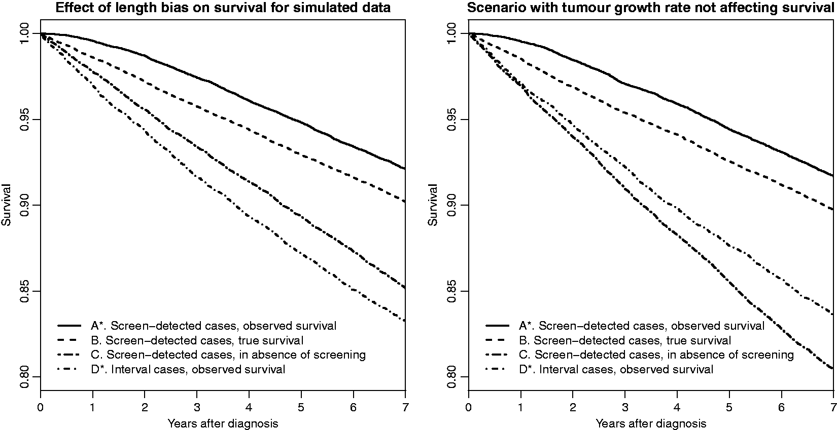

In the lower-right section in Figure 5, we plot symptomatic size against inverse growth rate, for screening and interval cases separately (300 cases of each are randomly sampled to aid visibility). The marginal medians (calculated from all, around 34,000, simulated cases) in the two groups are plotted as grey solid (interval cases) and black dashed (screening cases) lines. Screening cases have a larger median symptomatic tumour size than interval cases, even though interval cases are faster-growing, and fast growth is associated with a larger symptomatic size.³⁸ This difference in symptomatic size between screening and interval cases is even larger within groups with similar (conditional) growth rates.

It is also possible to simulate scenarios (using other parameter values) where the median symptomatic size is larger for interval cases than for screening cases (not conditioning on growth rate). This can be done, for example, if the growth rate distribution among all breast cancers is made to be more heterogeneous, leading to larger differences in growth rates between screen and interval cases. In Figure 8 in Appendix 3 we show the same plots as in Figure 5, but for a simulation under this scenario (in which τ₁ = 1, τ₂ = 2, η = e^−7.50). We discuss this scenario further in Section 5.1.

Figure 7.

Survival comparison on Swedish postmenopausal breast cancer cases corrected for lead time bias but not length bias.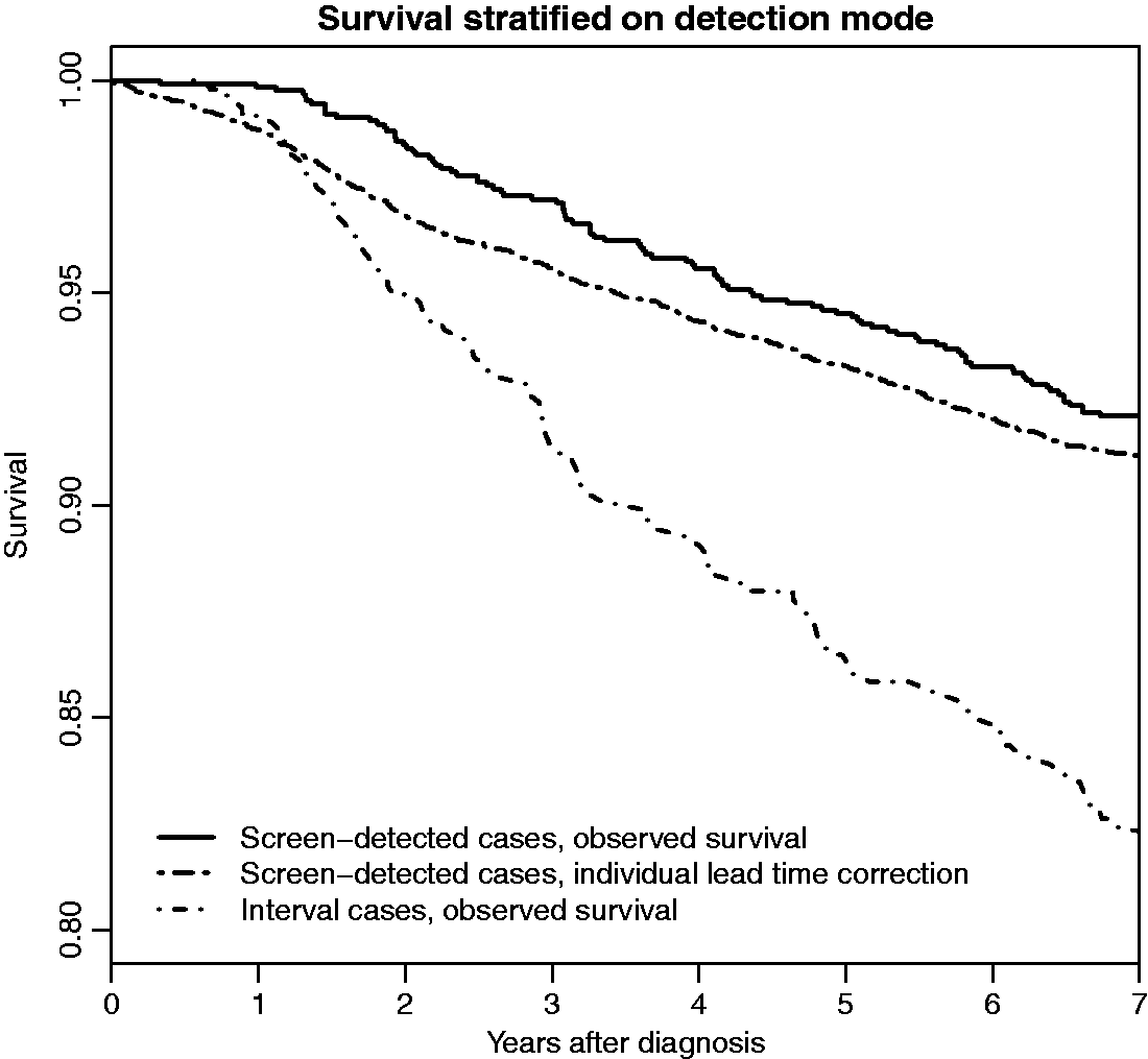

Using our simulation study we have shown that there is an effect of length-biased sampling of screening cases, not only on tumour growth rate, but also on the symptomatic tumour size. This has, to our knowledge, not been shown before.

5 Length bias and effect of screening on survival comparisons

We now turn to discussing the effect of length bias (and lead time bias) on survival comparisons. In Section 5.1 we exemplify the biases on simulated data along with an illustrative example on observational data. In Section 5.2 we discuss existing real data analyses in the cancer screening literature and mention other biases that may arise in survival comparisons. We also suggest a strategy for jointly correcting for lead time and length biases (Section 5.3).

5.1 Survival comparisons on simulated data

We use our data simulation (with τ₁ = 2.36, τ₂ = 3.00, η = e^−8.75, λ = 6⋅10⁻⁴ and γ = 4⋅10⁻³) to exemplify the impact of the lead time and length biases on survival comparisons across subgroups of cases defined on detection mode and screening history. In our simulation, subgroups are defined on screening/interval status, which is defined under our simulated scenario of screening, although when plotting survival times we measure survival from diagnosis both under screening and under the counterfactual scenario of no screening. Screening cases will have a screen and a symptomatic diagnosis and, after symptomatic diagnosis, will have different survival times under the presence and absence of screening, since in the presence of screening their survival times are generated using a different tumour size than in the absence of screening, see equation (10). We recall that overdiagnosed cancers are uncommon in our simulated data and that all women attend screening. To ease understanding, overdiagnosis and non-adherence to screening are not discussed further in this section. Let us start by defining seven sets of individuals and survival times, labelled A-G, which we will use to help explain the biases and the effects of screening. Some of these survival times for these defined groups of individuals are observable and some are not, for a population in which screening is offered. The sets of survival times (for the particular individuals) which are observable are marked with an asterisk (*).

Survival times for screen-attending invasive breast cancer cases

A*. Screening cases only, in the presence of screening, measured from screen diagnosis.

B. Screening cases only, in the presence of screening, measured from symptomatic diagnosis.

C. Screening cases only, in the absence of screening, measured from symptomatic diagnosis.

D*. Interval cases only, in the presence of screening, measured from symptomatic diagnosis.

E*. All cases, in the presence of screening, measured from observed diagnosis.

F. All cases, in the presence of screening, measured from symptomatic diagnosis.

G. All cases, in the absence of screening, measured from symptomatic diagnosis.

A* and D* represent survival times for screen and interval detected cases, respectively, which are usually observable in data collected in the presence of a screening programme (as long as information on screening history and detection mode is available). B and C represent the lead time corrected (true lead time is known in the simulation) survival times for screening cases as if they, respectively, were and were not, screened. These two survival times are measured from the same time point, the time of symptomatic detection, but the former includes an effect of screening (i.e. of being treated from the time point of screen detection) whilst the latter does not (i.e. being treated from the symptomatic detection).

Comparing different sets of individuals and survival times will shed light on different combinations of the effects of lead time bias, length bias and of attending/being detected at screening. These are summarised as follows.

Differences in survival times for screen-attending invasive breast cancer cases

Differences in A* and D* are due to lead time bias, length bias, and the effect of being screen-detected.

Differences in A* and B are due to lead time bias.

Differences in A* and C are due to lead time bias and the effect of being screen-detected.

Differences in B and D* are due to length bias and the effect of being screen-detected.

Differences in B and C are due to the effect of being screen-detected

Differences in C and D* are due to length bias.

Differences in E* and F are due to lead time bias.

Differences in E* and G are due to lead time bias and the effect of attending screening.

Differences in F and G are due to the effect of attending screening

Differences in C and G are due to length bias.

Differences in D* and G are due to length bias.

In a simulation with all (natural history, screening sensitivity and survival model) parameters, we can construct all curves and make comparisons. However, based on observational data, there are no two typically observable survival curves which can be compared in order to retrieve the (unbiased) effect of screening. We would rather typically need to compare two non-observable survival time distributions, such as B and C (to retrieve the effect of being detected at screening) or F and G (to retrieve the effect of attending a screening programme). To evaluate unbiasedly the effect of using a screening programme at a population level (that is, the effect of invitation to a screening programme, when full adherence to screening is not assumable), one needs to compare F and G (but both groups would need to include non-attenders). Using our lead time correction, it would be possible to estimate both curves B and F from observational data. However, approaches for estimating C and G remain to be described. G is observable in populations not offering screening; however, comparing populations with and without screening will often lead to other biases arising, for reasons which we discuss in Section 5.2.

Some plots of survival times for (A–D), based on our simulation, are shown in Figure 6. The plot to the left is based on the same natural history and survival parameters as in Figures 2 to 5. Differences between curves C and D* reflect length bias, whilst differences between curves B and C are due to effects of women being detected at screening (if the interval cases would have had other screening time points and been screen-detected they would not have experienced the same screen effect). In the panel to the right of Figure 6, we show survival curves A–D for an alternative simulation in which γ (the coefficient for inverse tumour growth rate in the time to death functions (10)) is set to 0 and λ (the coefficient for tumour size at diagnosis) is increased (to 1.2⋅10⁻³) in order to compensate and make the overall survival similar to that in the left panel. With γ = 0 there is no effect of growth rate on survival, but a length bias still exists (curves C and D*), since the symptomatic tumour size distributions differ between screening and interval cases; see Figure 5. In this simulation the length bias goes in the opposite direction from that expected according to the classical view of length bias, i.e. screening cases have worse survival than interval cases in the absence of screening, since the median symptomatic tumour size is larger for screening cases than for interval cases. If we had inserted a small effect of growth rate on survival, then it is possible that the length bias (difference between curves C and D*) would have disappeared. It is thus evident that a non-existing length bias does not necessarily imply that growth rate does not affect survival. We discuss this further in Section 5.2.

Using the previously mentioned simulated data set with an increased growth rate heterogeneity (see Figure 8 in Appendix 3) in which interval cases have a larger median symptomatic tumour size than screening cases, it is, in any case, possible to produce a scenario where interval cases have worse survival than screening cases (comparing curves C and D*), although growth rate has no effect on survival; see Figure 9 in Appendix 3. To make the overall survival similar to the one in Figure 6, survival parameter values for time to death functions (10) were set to $λ = 1.1 \cdot 10^{- 3}$ and γ = 0.

Figure 8.

Distributions (as if screening was not present) of tumour presence time, inverse growth rate and symptomatic size (and marginal medians for the two last quantities) from simulated data, by detection mode (screening/interval), in the presence of screening. Based on growth rate parameter values τ₁ = 1, τ₂ = 2 and symptomatic detection parameter value, η = e^−7.50.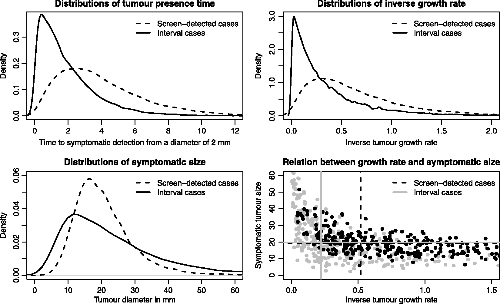

For illustrative purposes, we show, in Figure 7, curves A*, B and D* for the 1745 breast cancer cases described in Section 4.1. For the individual lead time correction, 10 conditional lead time values were sampled for each woman to decrease variability in the correction procedure. It can be seen that it is unlikely that the lead time bias explains a large proportion of the survival difference between screen-detected and interval cases. The lead time bias appears to be larger in survival comparisons closer to the diagnosis date, than later.

5.2 Examples of survival comparisons based on real, observational data

In the cancer screening literature, different selections of particular curves (from those defined in Section 5.1) have been constructed from observational data to draw conclusions about the effect of screening and the magnitude of length bias. Duffy et al.¹⁸ tried to construct survival curves for A*, B and a variant of D*, from large observational data of breast cancer cases diagnosed between 1988 and 2004 in the United Kingdom. They compared observed survival for screening cases, and estimated lead time corrected survival for screening cases, and survival for interval cases and non-attenders grouped together. These authors accounted for lead time bias using the average method. There are a number of difficulties associated with using these curves to evaluate the effect of being screen-detected on survival. Interval cases have been reported by Lawrence et al.³⁹ to have a better survival than women not attending screening in this data, which could hypothetically be due to, e.g., treatment compliance. This bias was, however, addressed by Lawrence et al.² in an analysis of the same data set in which lead time corrected survival for screening cases (B) was compared to survival for interval cases (D*). The difference in survival between interval cases and non-attenders may, however, differ between national screening programmes, and will be affected by, for example, screening sensitivity and treatment adherence heterogeneity between groups in the population. In the comparison of survival curves B and D*, contributions of length bias and overdiagnosis also need to be accounted for before assessing screening effects. In part, their contributions can be removed by excluding in situ cancers. In Lawrence et al.'s² analysis with this exclusion, 10-year survival was estimated to be 81% and 72% for screening and interval cases, respectively. To address length bias, these authors performed a sensitivity analysis (using an approach described in Duffy et al.¹⁸). Their analysis is, however, somewhat ad-hoc: it places boundaries on the magnitude of the length bias by using an assumption that women with fast-growing tumours will have at most a two times higher risk of dying from breast cancer during the follow-up time compared to women with slow-growing tumours. They also assumed growth rate to be categorical with two levels. There may also be calendar period effects included in their results (if the fraction of screening to interval cases was changing over time) that are not accounted for. Women diagnosed in 2004 are likely to have, on average, longer survival times than women diagnosed in 1988 due to improved treatments. Such an effect may favour the survival times of interval cases since more screening cases will be detected among prevalent cases at the first screen occasion (the screening programme was launched in 1988), or be in favour of screening cases if screening sensitivity has continually increased over time. A calendar period effect on relative survival times has, for example, been shown by Saadatmand et al.⁴⁰ in data collected between 1999 and 2012 in the Netherlands. Lawrence et al.³⁹ also show that survival has improved over time mostly for the interval cases, thus an estimate of the effect of being screen-detected, excluding the earliest years would be of interest.

Kalager et al.⁴¹ compared survival times for interval cases (curve D*) to survival times for a non-screened population (a variant of curve G) in Norwegian data of cases diagnosed between 1996 and 2005, with one of the purposes being to evaluate length bias. The comparison was possible since screening was introduced gradually. The fact that interval cases had an almost identical survival to the non-screened population, in their data, was considered as evidence of no length bias. Referring to Kalager et al.'s analysis, Adami et al.⁴² concluded that tumour growth rate is not associated with survival. We believe that this conclusion should not be drawn. After all, in their data, interval cases had larger tumours than non-screened cases – using similar reasoning would lead us to conclude that survival times are not associated with tumour size. It is possible, or even likely, that other factors have influenced their result. (The result also does not tell us whether there exists a length bias in survival comparisons between screening and symptomatic cases, since there could be overdiagnosed women included among screen-detected cases.) The two groups are likely to be non-exchangeable since, for instance, among interval cases, only attenders of screening are included, whilst in the other group it is reasonable to assume that there exists a fraction that would not adhere to screening. If it were possible to exclude women who do not adhere to screening, the survival for the non-screened population would increase – the survival for interval cases would be worse than in the non-screened population. With such a result we would conclude that there exists a length bias. It would, however, not be easy to tell how much of the difference was due to differences in tumour growth rate distributions and/or symptomatic tumour size distributions. Also, individuals in the non-screened population are likely to be diagnosed at earlier time points than interval cases, thus there is a possible calendar time effect.

To assess the effect of inviting women to a screening programme in data sets similar to the Norwegian, one could compare (lead time corrected) survival for all women invited to screening to the survival for the non-screened population. The calendar time effect would be smaller in this study where screening was introduced gradually than in studies in which screening was introduced for all individuals at the same time. This type of analysis (but for mortality) was performed by Hanley et al.⁴³ for Irish data of cases diagnosed between 2000 and 2013. In Ireland, screening was introduced between 2000 and 2007, at different times within different regions. The study, however, suffered from a short follow-up period.

5.3 An approach for correcting for length bias and assessing the effect of screening in observational data

Although it is possible to assess the effect of screening using simulation (comparing a screening scenario to a counterfactual no screening scenario) if all natural history, screening sensitivity and survival model parameters are known, it remains a challenge to evaluate screening effects on survival from observable survival curves. Our aim is to be able to compare survival curves F and G (i.e. to compare lead time corrected survival for all cases following the screening programme, to survival for the same group of women as if screening had not been present). In Section 4.3 we showed how to construct a lead time corrected survival curve. We now make use of our earlier described simulation scenario in which only tumour size at detection and inverse tumour growth rate affect the risk of dying from breast cancer, to suggest an approach for estimating the effect of following a screening programme on survival.

To estimate G (that is, the unobserved survival for all cases following screening, as if screening was not present) we suggest to assume that the survival for symptomatic (interval) cases in the presence of screening will be the same as in the absence of screening, thus curve G needs to be estimated only for the screening cases. One can then include all cases (both screening and interval detected ones) and regress uncorrected (for lead time) survival on the value of tumour size at diagnosis, along with an estimate of growth rate from the conditional inverse tumour growth rate distribution of each woman. For screening cases we derive the conditional inverse tumour growth rate distribution (see Appendix 2) and note that it is also possible to derive this distribution for symptomatic cases. It would then be possible to predict a new survival time, from the time point of the theoretical symptomatic diagnosis, (to use for curve G) for each screening case based on the regression model by using an estimated value for the woman's symptomatic size in place of the observed tumour size at diagnosis. The conditional distribution for symptomatic tumour size could be derived from the conditional lead time distribution together with the conditional inverse tumour growth rate distribution. In our simulation we have used a simple model. In a real setting, not only tumour size and growth rate affect survival. Breast cancer is a heterogeneous disease and a number of factors affect survival and detection of tumours.

To calculate the effect of inviting women to screening on survival, instead of the effect of attending screening on survival (i.e. comparing variants of the curves F and G), one would follow the same procedure as above for the calculations. For the presentation, the survival times for the group of non-attenders would be included in both curves F and G.

If the effect of being screen-detected (comparing curves B and C) were to be estimated, the same procedure could be used (interval cases would still be needed for the regression model). Although we have here sketched out a procedure for correcting for length bias based on the continuous growth model, exact details still need to be worked out.

6 Discussion

In this article we have used a biological model of tumour growth to derive conditional lead time distributions, and have shown how these can be used on simulated and observational data to correct survival curves for lead time bias on an individual basis.

As well as being useful for correcting for bias in survival comparisons, the individual/conditional lead time distributions described in this article may be useful for determining, e.g., optimal individual screening intervals in an individualised screening programme. For understanding tumour heterogeneity and screening sensitivity, several researchers have tried to sub-divide interval cancers (into e.g. missed and true interval cancers), by, for example, categorising according to mammographic density.⁴⁴ The methodology described herein will be useful for making such sub-divisions in a more formal, and possibly more appropriate, way.

The conditional lead time distributions, described in this paper, open up new possibilities for analyses of observational screening data. They can be used, e.g., for estimating, in retrospect, how likely it was that a (screen-detected) breast cancer case, who died from a cause other than breast cancer, was overdiagnosed. With some further methodological development it may even be possible to predict, prospectively, at an individual level, the probability for a woman newly diagnosed with cancer (through screening) to be an overdiagnosed case. For this, a joint model for tumour characteristics and survival based on a continuous tumour growth model would be needed; see Chen et al.⁴ and Lee et al.¹² for related work on multi-state Markov models.

In our simulations, it is evident that the lead times are shorter than those in Duffy et al.,¹⁸ but more in line with the estimates presented by Chen et al.¹⁵ We have argued that the difference partly arises from the memoryless assumption of the multi-state Markov models. Also, the parameter values used by Duffy et al. were estimated from data on all breast cancers whereas the parameter values used in this paper were obtained from data only on invasive breast cancers. Nevertheless, inconsistencies in estimates of mean sojourn times are common in the breast cancer literature. For example Shen and Zelen reported estimates ranging from 1.9 to 4.3 years in four different large screening trials.⁴⁵ More, large studies are thus needed to estimate parameters of natural history models and to compare continuous growth models and multi-state Markov models.

The proposed lead time bias correction in this paper, without including a joint correction for length bias, may already be useful for some studies, e.g. for assessing the effect of being invited to screening on survival, by comparing curves F (including attenders and non-attenders of screening) to G, where the latter is observable. Examples of studies which could be used are the randomised trials and observational studies (Kalager et al.,⁴¹ Hanley et al.⁴³) where screening has been introduced gradually – provided that information on tumour size, screening history and detection mode is available. In analyses of any such data it would still be important to acknowledge biases arising from calendar time and regional differences.

Effects of screening are likely to differ across countries due, for example, to differences in attendance rates, treatment adherence, screening sensitivities, ages invited, screening intervals, underlying risks of getting the disease and disease heterogeneity. To assess the effectiveness of screening (the effect of being invited, the effect of attending, or the effect of being screen-detected, on survival) using observational data sets, a correction for length bias is needed. In this paper, we have discussed ways forward for creating such a correction, by predicting breast cancer survival in the whole population, or among the screening cases, as if screening would not have been present.

The fact that length bias is affected by both the tumour growth rate and the symptomatic tumour size, has a bearing on how observable breast cancer survival curves should be interpreted. Differences in tumour size distributions among screening and interval cases may not entirely be due to earlier detection through screening (as assumed in e.g. Allgood et al.³ with respect to tumour stage), but also may be due to length-biased sampling – this incorrect assumption was used to conclude that the stage shift explained most of the survival advantage seen in screening cases, and that length bias did not play a large role.

Continuous tumour growth models are very different to multi-state Markov models. Since the former have a closer link to biology (by for instance separating sojourn times into growth rate and symptomatic detectability) they open up for a greater understanding of etiology, which will be useful for developing individualised screening programmes. It has also been shown that there are simple ways to include risk factors into the different submodels of a continuous tumour growth model,⁴⁶ and computational difficulties are being addressed.²⁵ Further development of continuous growth models is needed to make them more realistic, e.g. to include lymph node and distant metastatic spread. The more accurate a natural history model is, the better it will be for correcting for lead time bias, length bias and overdiagnosis. In this paper, we have shown that continuous growth models can be used as a powerful tool to correct for, and increase knowledge of such biases.

Footnotes

Declaration of conflicting interests

The author(s) declared no potential conflicts of interest with respect to the research, authorship, and/or publication of this article.

Funding

The author(s) disclosed receipt of the following financial support for the research, authorship, and/or publication of this article: This work was supported by the Swedish Research Council [grant number 2016‐01245], the Swedish Cancer Society [grant number CAN 2017/287] and the Swedish e‐Science Research Centre. KC was supported by Stockholm County Council [grant number 20170088].

References

Independent UK Panel on Breast Cancer Screening. The benefits and harms of breast cancer screening: an independent review. Lancet 2012; 380: 1778–1786.

Lawrence

Wallis

Allgood

, et al. Population estimates of survival in women with screen-detected and symptomatic breast cancer taking account of lead time and length bias. Breast Cancer Res Treat 2009; 116: 179–185.

Allgood

Duffy

Kearins

, et al. Explaining the difference in prognosis between screen-detected and symptomatic cancers. Br J Cancer 2011; 104: 1680–1685.

Chen

Yen

AMF

Tabár

. A stochastic model for calibrating the survival benefit of screen-detected cancers. J Am Stat Assoc 2012; 107: 1339–1359.

Shen

Yang

Inoue

LYT

, et al. Role of detection method in predicting breast cancer survival: analysis of randomized screening trials. J Natl Cancer Inst 2005; 97: 1195–1203.

Vieira

de Senna

Harper

, et al. Tumour doubling times and the length bias in breast screening programmes. Health Care Manag Sci 2011; 14: 203–211.

Cox

Sneid

. Bias in breast cancer research in the screening era. Breast 2013; 22: 1041–1045.

Duffy

Day

Tabár

, et al. Markov models of breast tumor progression: some age-specific results. J Natl Cancer Inst Monogr 1997, pp. 93–97.

Duffy

Chen

Tabar

, et al. Estimation of mean sojourn time in breast cancer screening using a Markov chain model of both entry to and exit from the preclinical detectable phase. Stat Med 1995; 14: 1531–1543.

10.

Tan

KHX

Simonella

Wee

, et al. Quantifying the natural history of breast cancer. Br J Cancer 2013; 109: 2035–2043.

11.

Taghipour

Banjevic

Miller

, et al. Parameter estimates for invasive breast cancer progression in the Canadian National Breast Screening Study. Br J Cancer 2013; 108: 542–548.

12.

Lee

Huang

, et al. The Dana-Farber CISNET model for breast cancer screening strategies: an update. Med Decis Making 2018; 38: 44S–53S.

13.

Uhry

Hédelin

Colonna

, et al. Multi-state Markov models in cancer screening evaluation: a brief review and case study. Stat Methods Med Res 2010; 19: 463–486.

14.

Weedon-Fekjær

Tretli

Aalen

. Estimating screening test sensitivity and tumour progression using tumour size and time since previous screening. Stat Meth Med Res 2010; 19: 507–527.

15.

Chen

Brock

. Estimating key parameters in periodic breast cancer screeningapplication to the Canadian national breast screening study data. Cancer Epidemiol 2010; 34: 429–433.

16.

Rosner

Broemeling

. Bayesian inference for the lead time in periodic cancer screening. Biometrics 2007; 63: 873–880.

17.

de Koning

Draisma

Fracheboud

, et al. Overdiagnosis and overtreatment of breast cancer – microsimulation modelling estimates based on observed screen and clinical data. Breast Cancer Res 2006; 8: 202.

18.

Duffy

Nagtegaal

Wallis

, et al. Correcting for lead time and length bias in estimating the effect of screen detection on cancer survival. Am J Epidemiol 2008; 168: 98–104.

19.

Atkinson

Bartoszyński

Brown

, et al. On estimating the growth function of tumors. Math Biosc 1983; 67: 145–166.

20.

Brown

Atkinson

Bartoszynski

, et al. Estimation of human tumor growth rate from distribution of tumor size at detection. J Natl Cancer Inst 1984; 72: 31–38.

21.

Bartoszyński

Edler

Hanin

, et al. Modeling cancer detection: tumor size as a source of information on unobservable stages of carcinogenesis. Math Biosc 2001; 171: 113–142.

22.

Plevritis

Salzman

Sigal

, et al. A natural history model of stage progression applied to breast cancer. Stat Med 2007; 26: 581–595.

23.

Weedon-Fekjær

Lindqvist

Vatten

, et al. Breast cancer tumor growth estimated through mammography screening data. Breast Cancer Res 2008; 10: R41.

24.

Abrahamsson

Humphreys

. A statistical model of breast cancer tumour growth with estimation of screening sensitivity as a function of mammographic density. Stat Methods Med Res 2016; 25: 1620–1637.

25.

Isheden

Humphreys

. Modelling breast cancer tumour growth for a stable disease population. Stat Methods Med Res 2017. DOI: 10.1177/0962280217734583.

26.

Talkington

Durrett

. Estimating tumor growth rates in vivo. Bull Math Biol 2015; 77: 1934–1954.

27.

Spratt

von Fournier

Spratt

, et al. Decelerating growth and human breast cancer. Cancer 1993; 71: 2013–2019.

28.

Törnberg

Kemetli

Ascunce

, et al. A pooled analysis of interval cancer rates in six European countries. Eur J Cancer Prev 2010; 19: 87–93.

29.

Thomas

. Estimating the effect of targeted screening strategies: an application to colonoscopy and colorectal cancer. Epidemiol 2017; 28: 470–478.

30.

Magnusson

Baron

Persson

, et al. Body size in different periods of life and breast cancer risk in post-menopausal women. Int J Cancer 1998; 76: 29–34.

31.

Rosenberg

Granath

Dickman

, et al. Menopausal hormone therapy in relation to breast cancer characteristics and prognosis: a cohort study. Breast Cancer Res 2008; 10: R78.

32.

Eriksson

Czene

Rosenberg

, et al. The influence of mammographic density on breast tumor characteristics. Breast Cancer Res Treat 2012; 134: 859–866.

33.

Eriksson

Czene

Rosenberg

, et al. Mammographic density and survival in interval breast cancers. Breast Cancer Res 2013; 15: R48.

34.

The National Board of Health and Welfare. Statistics database for cancer, http://www.socialstyrelsen.se/statistik/statistikdatabas/cancer (accessed 22 October 2018).

35.

Forastero

Zamora

Guirado

, et al. A Monte Carlo tool to simulate breast cancer screening programmes. Phys Med Biol 2010; 7: 5213–5229.

36.

Statistics Sweden. Statistical database on mortality, http://www.statistikdatabasen.scb.se (accessed 22 October 2018).

37.

de Azambuja

Cardoso

de Castro Jr

, et al. Ki-67 as a prognostic marker in early breast cancer: a meta-analysis of published studies involving 12 155 patients. Br J Cancer 2007; 96: 1504–1513.

38.

Sigurdsson

Baldetorp

Borg

, et al. Indicators of prognosis in node-negative breast cancer. New Engl J Med 1990; 322: 1045–1053.

39.

Lawrence

O'Sullivan

Kearins

, et al. Screening histories of invasive breast cancers diagnosed 1989–2006 in the West Midlands, UK: variation with time and impact on 10-year survival. J Med Screen 2009; 16: 186–192.

40.

Saadatmand

Bretveld

Siesling

, et al. Influence of tumour stage at breast cancer detection on survival in modern times: population based study in 173 797 patients. BMJ 2015; 351: h4901.

41.

Kalager

Tamimi

Bretthauer

, et al. Prognosis in women with interval breast cancer: population based observational cohort study. BMJ 2012; 345: e7536.

42.

Adami

Csermely

Veres

, et al. Are rapidly growing cancers more lethal?. Eur J Cancer 2017; 72: 210–214.

43.

Hanley

Hannigan

O'Brien

. Mortality reductions due to mammography screening: contemporary population-based data. PLoS One 2017; 12: e0188947.

44.

Holm

Humphreys

, et al. Risk factors and tumor characteristics of interval cancers by mammographic density. J Clin Oncol 2015; 33: 1030–1037.

45.

Shen

Zelen

. Screening sensitivity and sojourn time from breast cancer early detection clinical trials: mammograms and physical examinations. J Clin Oncol 2001; 19: 3490–3499.

46.

Abrahamsson

Czene

Hall

, et al. Breast cancer tumour growth modelling for studying the association of body size with tumour growth rate and symptomatic detection using case-control data. Breast Cancer Res 2015; 17: 116.

Continuous tumour growth models,lead time estimation and length bias in breast cancer screening studies

Abstract

Keywords

1 Introduction

2 A continuous tumour growth model

3 Conditional lead time distributions

3.1 Calculations of conditional lead time distributions

3.2 Heterogeneity of lead time distributions in breast cancer

4 Lead time bias corrections and length bias – a simulation study and an illustrative example using Swedish (invasive) breast cancer data

4.1 Swedish postmenopausal breast cancer data

4.2 Data simulation procedure

4.3 A lead time correction based on conditional lead time distributions

4.4 Comparing individual and average lead time corrections using simulated data

4.5 Effect of the memoryless assumption in multi-state Markov models on lead times

4.6 A novel view on length bias

5 Length bias and effect of screening on survival comparisons

5.1 Survival comparisons on simulated data

Survival times for screen-attending invasive breast cancer cases

Differences in survival times for screen-attending invasive breast cancer cases

5.2 Examples of survival comparisons based on real, observational data

5.3 An approach for correcting for length bias and assessing the effect of screening in observational data

6 Discussion

Footnotes

Declaration of conflicting interests

Funding

References