Sage Journals: Discover world-class research

Abstract

Continuous growth models show great potential for analysing cancer screening data. We recently described such a model for studying breast cancer tumour growth based on modelling tumour size at diagnosis, as a function of screening history, detection mode, and relevant patient characteristics. In this article, we describe how the approach can be extended to jointly model tumour size and number of lymph node metastases at diagnosis. We propose a new class of lymph node spread models which are biologically motivated and describe how they can be extended to incorporate random effects to allow for heterogeneity in underlying rates of spread. Our final model provides a dramatically better fit to empirical data on 1860 incident breast cancer cases than models in current use. We validate our lymph node spread model on an independent data set consisting of 3961 women diagnosed with invasive breast cancer.

Keywords

Breast cancer tumour growth model joint modelling lymph node spread random effects modelling screening

1 Introduction

Since its popularisation in medical statistics, the multi-state Markov model has been the primary tool to model breast cancer progression using epidemiological or breast cancer screening data.^1–5 In recent years, however, several research groups have developed alternatives based on continuous processes. Bartoszynski et al.⁶ estimated tumour growth with an exponential growth function, explaining individual variation in growth rates with gamma distributed random effects. Plevritis et al.⁷ described some extensions of the model. Both of these early models based inference on tumour sizes of breast cancer cases in non-screened populations. Weedon-Fekjaer et al.^5,8 fitted a continuous tumour growth model to data collected from a screened population. They presented a parsimonious model, containing only four parameters, that described both tumour growth and screening sensitivity as continuous functions, enabling them to condition on screening history and mode of detection. An alternative approach that also uses screening data was described by Abrahamsson and Humphreys.⁹ The approach is based on specifying three underlying processes: tumour growth, screening sensitivity, and symptomatic detection. The authors essentially extended the model of Bartoszynski et al.⁶ and derived probability distributions for tumour sizes, conditioned on screening history and mode of detection. Isheden and Humphreys¹⁰ derived a number of mathematical results that simplified and reduced the computational complexity of the model.

The Markov model requires many parameters when the number of disease states is large. As a consequence, the model is not well suited for quantifying the role of individual risk factors on breast cancer progression. Continuous growth models, on the other hand, have few parameters, and can easily be modified to estimate tumour progression at an individual level. For example, Abrahamsson et al.¹¹ modelled tumour growth rate as a function of BMI and time to symptomatic detection as a function of breast size, and Abrahamsson and Humphreys⁹ and Isheden and Humphreys¹⁰ have estimated screening sensitivity as a continuous function of tumour and mammographic image-based covariates. For data collected in the absence of screening, Plevritis et al.⁷ extended the exponential growth model of Bartoszynski et al.⁶ with two disease states, representing regional lymph node spread and metastatic spread. In the presence of screening, no model that we know of has modelled both tumour growth and tumour spread as continuous time processes. The aim of this article is to develop such a joint process, based on the literature on lymph spread modelling and lymph spread simulation.

In 2000, the U.S National Cancer Institute established a consortium,¹² consisting of six research groups from Georgetown University, University of Texas MDACC, Dana-Farber Cancer Institute, Erasmus MC, Stanford University, and University of Wisconsin, to develop simulation-based modelling approaches for investigating the impact of breast cancer interventions, with a focus on prevention, screening, and treatment. Each group models the natural history of breast cancer as part of their investigation, and the last three groups model breast cancer tumour growth as a continuous time growth process. All groups model localised tumour stages, regionally spread stages, and distant metastatic stages, but only the University of Wisconsin group models breast tumour spread as a continuous time process.

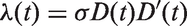
To model breast tumour spread, the Wisconsin group uses a model proposed by Shwartz,¹³ which assumes that tumour volume V grows exponentially with an individually assigned growth rate, and that the instantaneous rate of additional lymph node spread at time t is equal to $λ (t) = b_{1} + b_{2} V (t) + b_{3} V' (t)$ , where V(t) is tumour volume at time t, $V' (t)$ represents growth rate at time t, and b₁, b₂ and b₃ are constants. The group has modified the growth component slightly. They assume an exponential Gompertz function with decelerating doubling time. In fitting the model to observed breast cancer incidence data, the group found the overall model fit to be inadequate. When simulating lymph node progression and calibrating against U.S. breast cancer surveillance data, they found that the Shwartz model produced too much lymph node spread for large tumours. The model also generated too little lymph node spread for small tumours. Consequently, in order to improve fit, they made two ad-hoc adjustments to the model. First, they adjusted lymph node spread for large tumours by simulating spread based on tumour diameters 25% smaller than predicted by the growth model. Second, they assumed that 1% of all invasive tumours had four lymph nodes involved at tumour onset and that 2% had five or more lymph nodes involved.

Related tumour spread models have been proposed by Hanin and Yakovlev¹⁴ and, as mentioned, by Plevritis et al.⁷ Hanin and Yakovlev based their model on the model of Shwartz¹³ and assumed that tumours grow exponentially and that the rate of additional lymph node spread is proportional only to tumour volume. They introduced a number of additional assumptions and provided a detailed mathematical description of the model. Plevritis et al.⁷ described a simpler model. They assumed that the hazard of a localised tumour spreading to the lymph nodes is proportional to the volume of the tumour. They also relied on exponential tumour growth.

From the observations that: a) the CISNET University of Wisconsin group had to introduce additional assumptions to fit the Shwartz model to data and b) that the Shwartz model represents a generalisation of the models of Hanin and Yakovlev and Plevritis et al., we conclude that existing models can be improved upon. In this article, we back this claim by showing that the Shwartz model has two inherent weaknesses. The first weakness is that the model implies that slow growing tumours have a higher degree of lymph node spread, compared to fast growing tumours, and the second weakness is that the model implies either an unrealistically high degree of lymph node spread for large tumours or an unrealistically low degree of spread for small tumours. Based on these observations, there is a need for new statistical models of regional lymph node spread.

This article is structured in the following way. We present the models of Shwartz¹³ and Hanin and Yakovlev,¹⁴ and describe these weaknesses in detail. We then propose several models of regional lymph node spread. The first one is based on Shwartz¹³ but does not suffer the first weakness. The second one is a new model that addresses both of the weaknesses mentioned above. The new model assumes that the instantaneous rate of additional lymph node spread at time t, $λ (t)$ , is proportional to the number of times the tumour cells have divided at time t, D(t), and the rate of cell division in the tumour at time t, $D' (t)$ ,

λ (t) = σ D (t) D' (t)

Based on this, we propose a class of models in which every model avoids the weaknesses mentioned earlier, and show how our models can be modified to incorporate random effects to allow for heterogeneity in underlying rates of spread. We then describe a joint likelihood for tumour size and number of lymph nodes affected, given a patient's screening history and mode of detection. We use this likelihood to jointly estimate the tumour growth and lymph spread parameters from data on 1860 incident cases of breast cancer, collected from a population in which screening is offered. We show that our new models have superior model fit compared to the Shwarz-based model. In addition to showing that our new approaches provide better models of the mean, we show that incorporating random effects in the lymph node spread models further improves fit (dramatically so). We validate the lymph spread model on an independent data set consisting of 3961 women diagnosed with invasive breast cancer between January 2001 and December 2008 in the Stockholm-Gotland healthcare region in Sweden. We conclude with discussions of implications, strengths and weaknesses of the new models.

2 Traditional models of regional lymph node spread

Shwartz¹³ described a joint process for tumour growth and regional lymph node spread. Given an inverse growth rate r (assumed to vary across individuals), he assumed that tumour volume grows exponentially from time t = 0

V (t, r) = V_{0} e^{t / r}, t \geq 0

(1)

starting at an initial volume V₀, corresponding to a sphere of diameter

d_{0} = 0.5 mm

, and that the additional number of affected lymph nodes at time t follows an inhomogeneous Poisson process with intensity function

\begin{matrix} λ (t, r) = b_{1} + b_{2} V (t, r) + b_{3} V' (t, r) \end{matrix}

The model included additional assumptions. In what follows, we show that the first two assumptions alone imply that a tumour at volume V, with an inverse growth rate r, has higher expected lymph node spread than a faster growing tumour of the same size.

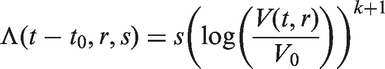
Based on the Poisson process proposed by Shwartz,¹³ it follows that the intensity measure is given by

\begin{matrix} Λ (t, r) = \int_{u = 0}^{t} λ (u, r) d u = b_{1} t + r b_{2} (V (t, r) - V_{0}) + b_{3} (V (t, r) - V_{0}) \end{matrix}

Given r and the tumour growth model (1), the time t is determined by

t = r (log V (t, r) - log V_{0})

. Substituting this into the first term of the above expression gives

\begin{matrix} Λ (t, r) = r b_{1} (log V (t, r) - log V_{0}) + r b_{2} (V (t, r) - V_{0}) + b_{3} (V (t, r) - V_{0}) \end{matrix}

For the inhomogeneous Poisson process, the intensity measure is the same as the expected value. Therefore, the expected number of affected lymph nodes at time t, given r, is

\begin{matrix} E [N | R = r, T = t] = Λ (t, r) \end{matrix}

Writing V = v, the expected number of lymph nodes affected, given R = r and V = v, is

\begin{matrix} E [N | R = r, V = v] = Λ (t (v), r) = r b_{1} (log (v) - log V_{0}) + r b_{2} (v - V_{0}) + b_{3} (v - V_{0}) \end{matrix}

From this expression, we can identify the first weakness: namely, for a given tumour volume, it follows that if r is large (slow growing) the expected number of affected lymph nodes is large, and when r is small (fast growing) the expected number of lymph nodes is small. This property is not supported by empirical evidence. If slow growing tumours would have a comparatively higher degree of lymph node spread, then screen detected cancers would have more lymph node involvement compared to interval cancers, due to length biased sampling. Empirical data show that this is not true (see end of Section 5).

Hanin and Yakovlev¹⁴ used the same tumour growth function, but assumed that the intensity function was given by $λ (t, r) = γ V (t, r)$ . Following the steps in the above argument for their model, the expected number of lymph nodes affected, given tumour volume and growth rate, is

E [N | R = r, V = v] = r γ (v - V_{0})

(2)

It follows that also their model is affected by the first weakness.

Both models, but especially the model of Hanin and Yakovlev, exhibit a second weakness. Namely, that the rate of additional lymph node spread increases enormously with increasing tumour volumes. We illustrate this by comparing the expected number of lymph nodes for tumours of diameters 5 mm and 30 mm. Plugging these diameters into equation (2), for fixed values of r and γ, we find that the expectation is more than 200 times larger for the bigger tumour. Such an extreme difference is not supported by clinical data. In our data the mean number of lymph nodes for 30 mm tumours (2.15) is less than nine times that for 5 mm tumours (0.25).

Shwartz¹³ found that when simulating cohorts of symptomatic cancers based on his model, he produced too few affected lymph nodes in tumours with diameters smaller than 1 mm. The CISNET University of Wisconsin group also saw this when using their modified approach. They also found that the model generated too many lymph nodes in large tumours. Even though the second weakness, strictly speaking, does not have to apply to the Shwartz model, it clearly does, as the findings of the two groups show. Together, these weaknesses mean that new models of lymph node spread are needed.

3 Joint processes of tumour growth and lymph node spread

In this section, we present joint processes of tumour growth, time to symptomatic detection, and lymph node spread. The joint processes share the same models for tumour growth, variation in tumour growth, and time to symptomatic detection, but differ in their models of lymph node spread. All models are, however, based on the same general framework: an inhomogeneous Poisson process with intensity function dependent on tumour volume. The first, called model A, is a variation of Shwartz,¹³ where we assume that the intensity function is proportional to the first derivative of tumour growth, $V'$ . Model B is biologically inspired, and assumes that the intensity function is proportional to the number of times the tumour cells have divided and the rate of cell division in the tumour. Lastly, we present a larger class of models based on model B. In what follows, we describe the shared models, the shared modelling assumptions, and give detailed descriptions of the proposed lymph spread models.

3.1 Shared processes and assumptions

We use the original tumour growth process that Schwartz¹⁵ described in 1961, and adopt the other shared models from Bartoszynski et al.,⁶ Hanin and Yakovlev,¹⁴ Plevritis et al.,⁷ Abrahamsson and Humphreys,⁹ and Isheden and Humphreys.¹⁰

We assume that the tumour is monoclonal and originates from a spherical cell of diameter $d_{Cell} =$ 10 µm, with corresponding volume $V_{Cell}$ . The tumour grows exponentially at a constant cell reproductive rate, here represented by the inverse growth rate r; the volume of the tumour t years after its onset is specified by

V (t, r) = V_{Cell} e^{t / r}, t \geq 0

(3)

We explain individual variation in growth rate with a gamma distribution of shape τ₁ and rate τ₂

f_{R} (r) = \frac{τ_{2}^{τ_{1}}}{Γ (τ_{1})} r^{τ_{1} - 1} e^{- τ_{2} r}, r \geq 0

(4)

Lastly, we assume that the tumour can be detected with non-zero probability, either symptomatically or via screening, from size V₀, corresponding to a spherical tumour of diameter

d_{0} = 0.5 mm

, and that the rate of symptomatic detection at time

T_{\det} = t

is proportional to the size of the tumour

P (T_{\det} \in [t, t + dt) | T_{\det} \geq t, R = r) = η V (t, r) dt + O (dt), V (t, r) \geq V_{0}

(5)

These processes are assumed to be independent of lymph node spread, i.e. the tumour does not grow faster or slower as it spreads and symptomatic detection is not triggered by lymph node metastases.

We begin with the two models of spread which we call A and B. We then work in a stepwise fashion, developing model B to a class of models and then showing how these can be extended to incorporate random effects.

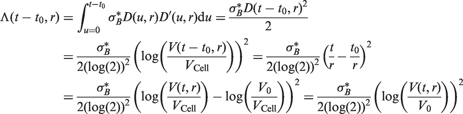
In all models, we assume that spread occurs one cell at a time and that secondary tumours (in the lymph nodes) have the same cell reproductive rate as the primary tumour. We only model spread that eventually becomes clinically detectable, i.e. lymph node spread that is detectable by the physician once the primary tumour has been detected. Secondary tumours need to grow to size V₀ to be clinically detectable (we could in theory use a volume different to V₀ here). This means that between the time of tumour spread and the time at which the secondary tumour becomes a clinically detectable lymph node metastasis, there is a time lag of size t₀. For a fixed inverse growth rate r, the time lag is defined by

V_{0} = V_{Cell} e^{t_{0} / r}

(6)

Given that secondary tumours are detectable first at size V₀, a lymph node metastasis that is clinically detectable at time t must have occurred between times zero and

t - t_{0}

, so that it has a volume greater than or equal to V₀ at time t. Thus, if the intensity measure is

Λ (t, r)

, the number of clinically detectable lymph nodes at time t is Poisson distributed with intensity measure

Λ (t - t_{0}, r)

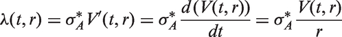
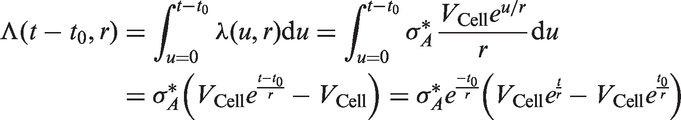
3.2 Model A

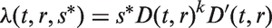
The first lymph node spread model is an inhomogeneous Poisson process with intensity function

\begin{matrix} λ (t, r) = σ_{A}^{*} V' (t, r) = σ_{A}^{*} \frac{d (V (t, r))}{dt} = σ_{A}^{*} \frac{V (t, r)}{r} \end{matrix}

The intensity measure at time

t - t_{0}

\begin{matrix} Λ (t - t_{0}, r) = \int_{u = 0}^{t - t_{0}} λ (u, r) d u = \int_{u = 0}^{t - t_{0}} σ_{A}^{*} \frac{V_{Cell} e^{u / r}}{r} d u \\ = σ_{A}^{*} (V_{Cell} e^{\frac{t - t_{0}}{r}} - V_{Cell}) = σ_{A}^{*} e^{\frac{- t_{0}}{r}} (V_{Cell} e^{\frac{t}{r}} - V_{Cell} e^{\frac{t_{0}}{r}}) \end{matrix}

Using equations (3) and (6) and introducing

σ_{A} = σ_{A}^{*} \frac{V_{Cell}}{V_{0}}

, the number of clinically detectable lymph nodes metastases at time T = t, given R = r, follows

\begin{matrix} P (N = n | R = r, T = t) = e^{- σ_{A} (V (t, r) - V_{0})} \frac{{(σ_{A} (V (t, r) - V_{0}))}^{n}}{n!} \end{matrix}

Given R = r and the tumour growth function (3), the time T = t is uniquely determined by the volume of the tumour. Writing V = v, the probability for N = n clinically detectable lymph nodes, given R = r and V = v, is

\begin{matrix} P (N = n | R = r, V = v) = e^{- σ_{A} (v - V_{0})} \frac{{(σ_{A} (v - V_{0}))}^{n}}{n!} \end{matrix}

(7)

The right hand side of equation (7) is independent of r. For model A, the probability for N = n clinically detectable lymph nodes, given volume V = v, is therefore

\begin{matrix} P (N = n | V = v) = e^{- σ_{A} (v - V_{0})} \frac{{(σ_{A} (v - V_{0}))}^{n}}{n!} \end{matrix}

(8)

Note that in the case of the two lymph spread models described in Section 2, given v, N is not conditionally independent of r.

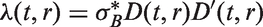
3.3 Model B

We now focus on deriving a biologically inspired model for lymph node spread. We base our model on two observations: A) lymphatic fluid is hostile to tumour cells; it contains little oxygen and nutrients, and tumour cells in the lymphatic system are under constant attack by the immune system. In order to survive, tumour cells entering the lymph system need to be highly mutated. B) Cell migration and cell proliferation share some common growth factors, such as the Hepatocyte Growth Factor/scatter factor.¹⁶ Thus, the rate of cancer spread may be related to the rate of cell division.

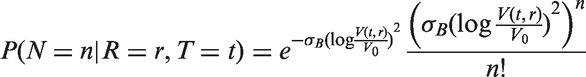
Based on A) and B), we assume that the rate of lymph node spread is proportional to the average number of mutations in the cancer cells and the rate of cancer cell division. The first of these quantities is not observable, but assuming a constant rate of mutation during cell division, the average number of mutations in the cancer cells is proportional to the number of times the cells in the tumour has divided. In summary, the second spread model is an inhomogeneous Poisson process with intensity function

λ (t, r) = σ_{B}^{*} D (t, r) D' (t, r)

where D(t, r) is the number of times the cells in the tumour has divided and

D' (t, r)

is the rate of cell division in the tumour – both at time t, assuming an inverse growth rate r.

Assuming that cancer cells form a spherical and densely packed tumour, and that cancer cells resist cell death, the number of times the cells in the tumour has divided is calculated by describing tumour volume as a doubling process. We get the number of cell divisions from the following relation

\begin{matrix} V_{Cell} \cdot 2^{D (t, r)} = V (t, r) \Leftrightarrow D (t, r) = \frac{log (\frac{V (t, r)}{V_{Cell}})}{log (2)} \end{matrix}

(9)

Using equations (3), (6), and (9), we derive the intensity measure at time

t - t_{0}

as follows

\begin{matrix} Λ (t - t_{0}, r) = \int_{u = 0}^{t - t_{0}} σ_{B}^{*} D (u, r) D' (u, r) d u = \frac{σ_{B}^{*} D {(t - t_{0}, r)}^{2}}{2} \\ = \frac{σ_{B}^{*}}{2 {(log (2))}^{2}} (log (\frac{V (t - t_{0}, r)}{V_{Cell}}))^{2} = \frac{σ_{B}^{*}}{2 {(log (2))}^{2}} (\frac{t}{r} - \frac{t_{0}}{r})^{2} \\ = \frac{σ_{B}^{*}}{2 {(log (2))}^{2}} (log (\frac{V (t, r)}{V_{Cell}}) - log (\frac{V_{0}}{V_{Cell}}))^{2} = \frac{σ_{B}^{*}}{2 {(log (2))}^{2}} (log (\frac{V (t, r)}{V_{0}}))^{2} \end{matrix}

Introducing

σ_{B} = \frac{σ_{B}^{*}}{2 {(log (2))}^{2}}

, the number of clinically detectable lymph nodes metastases at time T = t, given R = r, follows

\begin{matrix} P (N = n | R = r, T = t) = e^{- σ_{B} {(log \frac{V (t, r)}{V_{0}})}^{2}} \frac{(σ_{B} {(log \frac{V (t, r)}{V_{0}})}^{2}) n}{n!} \end{matrix}

\begin{matrix} P (N = n | R = r, V = v) = e^{- σ_{B} {(log \frac{v}{V_{0}})}^{2}} \frac{(σ_{B} {(log \frac{v}{V_{0}})}^{2}) n}{n!} \end{matrix}

(10)

As in model A, the right hand side of equation (10) is independent of r. Therefore, for model B, the probability for N = n clinically detectable lymph nodes, given volume V = v, is

\begin{matrix} P (N = n | V = v) = e^{- σ_{B} {(log \frac{v}{V_{0}})}^{2}} \frac{(σ_{B} {(log \frac{v}{V_{0}})}^{2}) n}{n!} \end{matrix}

(11)

3.4 A new class of models for lymph node spread

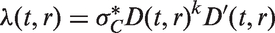
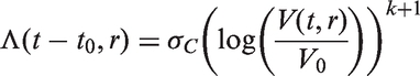
Based on model B, we here define a class of mathematically tractable models for lymph node spread. We show that if the intensity function is assumed to be proportional to the kth power of the number of cell divisions in the tumour and the rate of cell division in the tumour, and if we make the same assumptions as in model B, we can derive closed forms for $P (N = n | R = r, V = v)$ and $P (N = n | V = v)$ . These functional forms are harder to motivate. However, we note that if model fit would be better for a higher power of k, it could imply that lymph node spread depends on higher powers of tumour mutation or that breast cancer tumours mutate at an accelerating rate (referred to as genomic instability¹⁷.

We define the new model class, similarly to model B, by assuming that lymph node spread follows an inhomogeneous Poisson process with intensity function

λ (t, r) = σ_{C}^{*} D (t, r)^{k} D' (t, r)

where k is a number greater than minus one, t is time, r is the inverse growth rate of the tumour, D(t, r) is the number of times the cells in the tumour has divided, and

D' (t, r)

is the rate of cell division in the tumour. It follows that the intensity measure at time

t - t_{0}

Λ (t - t_{0}, r) = σ_{C} (log (\frac{V (t, r)}{V_{0}}))^{k + 1}

where

σ_{C} = \frac{σ_{C}^{*}}{(k + 1) {(log (2))}^{k + 1}}

. Similar to earlier, the probability for N = n clinically detectable lymph nodes, given R = r and V = v, is

P (N = n | R = r, V = v) = e^{- σ_{C} {(log \frac{v}{V_{0}})}^{k + 1}} \frac{(σ_{C} {(log \frac{v}{V_{0}})}^{k + 1}) n}{n!}

(12)

and the probability for N = n clinically detectable lymph nodes, given volume V = v, is

P (N = n | V = v) = e^{- σ_{C} {(log \frac{v}{V_{0}})}^{k + 1}} \frac{(σ_{C} {(log \frac{v}{V_{0}})}^{k + 1}) n}{n!}

(13)

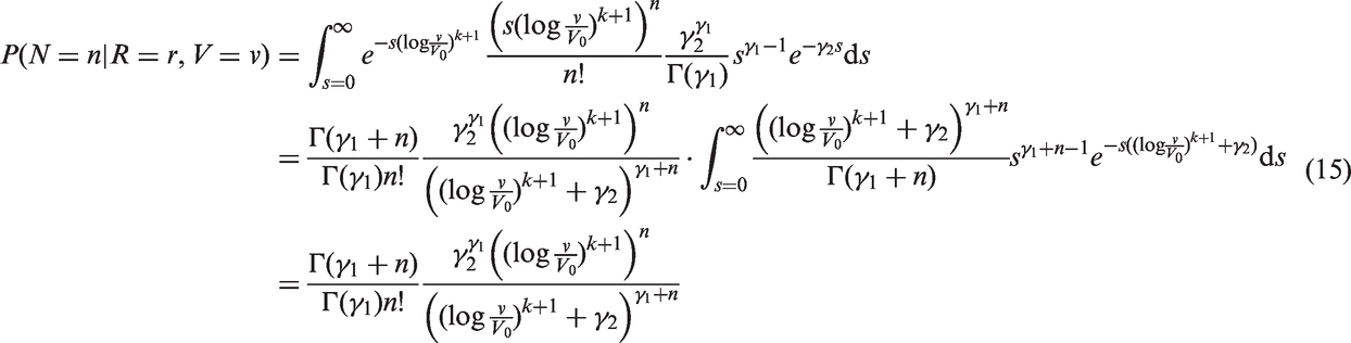
3.5 Random effects modelling of lymph node spread

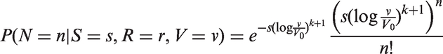
So far we have concentrated on developing new models of the mean numbers of affected lymph nodes. Breast cancer is, however, a heterogeneous disease; just as tumours grow at different speeds for different women, it would seem reasonable that breast cancer lymph node spread will occur at different rates for different women. We derive here a Poisson process where the constant factor s is gamma distributed. As before, we assume that

\begin{matrix} λ (t, r, s^{*}) = s^{*} D (t, r) k D' (t, r) \end{matrix}

It follows that the intensity measure at time

t - t_{0}

\begin{matrix} Λ (t - t_{0}, r, s) = s (log (\frac{V (t, r)}{V_{0}}))^{k + 1} \end{matrix}

where

s = \frac{s^{*}}{(k + 1) {(log (2))}^{k + 1}}

. Now, the probability for N = n clinically detectable lymph nodes, given S = s, R = r and V = v, is

P (N = n | S = s, R = r, V = v) = e^{- s {(log \frac{v}{V_{0}})}^{k + 1}} \frac{(s {(log \frac{v}{V_{0}})}^{k + 1}) n}{n!}

If we assume that s is gamma distributed with shape γ₁ and inverse scale γ₂

\begin{matrix} f_{S} (s) = \frac{γ_{2}^{γ_{1}}}{Γ (γ_{1})} s^{γ_{1} - 1} e^{- γ_{2} s}, s \geq 0 \end{matrix}

(14)

then it follows that the probability for N = n clinically detectable lymph nodes, R = r and V = v, is

\begin{matrix} P (N = n | R = r, V = v) = \int_{s = 0}^{\infty} e^{- s {(log \frac{v}{V_{0}})}^{k + 1}} \frac{(s {(log \frac{v}{V_{0}})}^{k + 1}) n}{n!} \frac{γ_{2}^{γ_{1}}}{Γ (γ_{1})} s^{γ_{1} - 1} e^{- γ_{2} s} d s \\ = \frac{Γ (γ_{1} + n)}{Γ (γ_{1}) n!} \frac{γ_{2}^{γ_{1}} ({(log \frac{v}{V_{0}})}^{k + 1}) n}{({(log \frac{v}{V_{0}})}^{k + 1} + γ_{2}) γ_{1} + n} \cdot \int_{s = 0}^{\infty} \frac{({(log \frac{v}{V_{0}})}^{k + 1} + γ_{2}) γ_{1} + n}{Γ (γ_{1} + n)} s^{γ_{1} + n - 1} e^{- s ({(log \frac{v}{V_{0}})}^{k + 1} + γ_{2})} d s \\ = \frac{Γ (γ_{1} + n)}{Γ (γ_{1}) n!} \frac{γ_{2}^{γ_{1}} ({(log \frac{v}{V_{0}})}^{k + 1}) n}{({(log \frac{v}{V_{0}})}^{k + 1} + γ_{2}) γ_{1} + n} \end{matrix}

(15)

As before,

P (N = n | R = r, V = v)

does not involve r, and therefore the probability for N = n clinically detectable lymph nodes, given S = s and V = v, is

\begin{matrix} P (N = n | V = v) = \frac{Γ (γ_{1} + n)}{Γ (γ_{1}) n!} \frac{γ_{2}^{γ_{1}} ({(log \frac{v}{V_{0}})}^{k + 1}) n}{({(log \frac{v}{V_{0}})}^{k + 1} + γ_{2}) γ_{1} + n} \end{matrix}

(16)

This probability follows a negative binomial distribution

NB (r, p)

with

r = γ_{1}

and

p = \frac{{(log \frac{v}{V_{0}})}^{k + 1}}{{(log \frac{v}{V_{0}})}^{k + 1} + γ_{2}}

4 Likelihood for incident cases in the presence of screening

To jointly estimate the parameters of the processes, we derive a likelihood function for incident breast cancer cases, collected in the presence of screening. This approach requires a model for mammography screening test sensitivity.

A screening test depends primarily on two factors: tumour size and mammographic density. Mammographic density reflects the different tissues in the breast. Fatty tissue appears dark on a mammogram, whereas fibroglandular tissue is bright. Since tumours also appear bright, they can be concealed in fibroglandular regions. A widely used measure of mammographic density is percentage density, which is measured as the fraction of pixels within the breast region on the mammogram that have an intensity above a particular threshold. 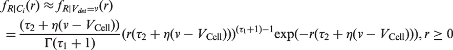For screening sensitivity, we adopt a model from Abrahamsson and Humphreys.⁹ We assume that the probability for a positive screening test, given a tumour in the breast, is equal to

\begin{matrix} S (d, m) = \frac{exp (β_{1} + β_{2} d + β_{3} m)}{1 + exp (β_{1} + β_{2} d + β_{3} m)}, d \geq 0.5 mm, 0 \leq m \leq 1 \end{matrix}

(17)

where d is the diameter of the tumour and m is percentage density of the breast. Implicitly, we assume that screening test sensitivity is independent of lymph node spread.

We can use the model for screening sensitivity, along with the other models, to write the joint likelihood of tumour size and number of lymph nodes affected, conditioning on screening history and mode of detection. Under stable disease assumptions^14,10 and assuming that tumour growth rate is independent of screening attendance, it has been shown that optimising this likelihood, using incident cases only, yields unbiased parameter estimation.¹⁰ The stable disease assumptions are

The rate of births in the population is constant across calendar time,

The distribution of age at tumour onset is constant across calendar time, and

The distribution of time to symptomatic detection is constant across calendar time.

These assumptions manifest in a constant incidence of breast cancer in the population. We discuss these assumptions in the light of our analysis in section 7.

Pathologists tend to round small tumour diameters to the nearest mm, and larger tumour diameters to the closest 5 or 10 mm. Therefore, we divide tumour sizes into 24 different millimetre size intervals, $[0.5, 1.5),$ $[1.5, 2.5),$ $[2.5, 7.5),$ $[7.5, 12.5),$ $\dots,$ $[67.5, 72.5),$ $[72.5, 85),$ $[85, 95),$ $\dots,$ $[145, 155)$ , and express the likelihood of those discrete size categories. Each likelihood is schematically written as

p_{i, j} = P (Size category i, j nodes affected | medical history)

where we use medical history to denote the time of tumour detection, the mode of detection, the number and time points of previous screening visits, and percentage mammographic density (conceptually, any type of medical history, such as previous use of hormone replacement therapy, could be included). In the following sections, we express the likelihood mathematically, using the following notation:

A – There is a tumour in the woman's breast at time t.

B₀ – A tumour is screen detected at time t.

$B^{c} = B_{1}^{c} \cap B_{2}^{c} \cap \dots \cap B_{n}^{c}$ – No tumour is detected at screenings 1 through n previous to detection (at $t_{1}, \dots, t_{n}$ years prior to time t).

C_i – The tumour is in size interval i at time t.

$C_{l, τ}$ – The tumour is in size interval l at τ years previous to time t.

D – The tumour is symptomatically detected at time t.

N_j – The number of lymph nodes affected at time t is j.

The likelihood is treated somewhat differently for screen detected and symptomatically detected cancers. For the sake of clarity, we omit mammographic density from the likelihood calculations.

4.1 Likelihood for screen detected cases

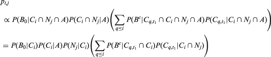
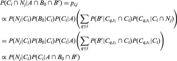
Given that a tumour is screen detected, the probability of the tumour being in size interval i with j lymph nodes affected is

p_{i, j} = P (C_{i} \cap N_{j} | A \cap B_{0} \cap B^{c})

(18)

We rewrite the probability algebraically, and use independence of screening test and lymph node status to get

\begin{matrix} p_{i, j} \\ \propto P (B_{0} | C_{i} \cap N_{j} \cap A) P (C_{i} \cap N_{j} | A) (\sum_{q \leq i} P (B^{c} | C_{q, t_{1}} \cap C_{i} \cap N_{j} \cap A) P (C_{q, t_{1}} | C_{i} \cap N_{j} \cap A)) \\ = P (B_{0} | C_{i}) P (C_{i} | A) P (N_{j} | C_{i}) (\sum_{q \leq i} P (B^{c} | C_{q, t_{1}} \cap C_{i}) P (C_{q, t_{1}} | C_{i} \cap N_{j})) \end{matrix}

where

i = 1, \dots, 24, j = 1, 2, \dots

, and

q = 0, \dots, i

. The value q = 0 represents a tumour that is too small to be clinically detectable, i.e. tumour diameter less than 0.5 mm. When there is no screen previous to detection, we omit the last summation from the product.

4.2 Likelihood for symptomatic cases

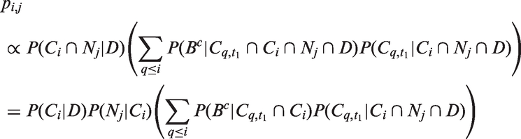
Given that a tumour is symptomatically detected, the probability of the tumour being in size interval i with j affected lymph nodes is

\begin{matrix} p_{i, j} = P (C_{i} \cap N_{j} | A \cap D \cap B^{c}) \end{matrix}

(19)

Similarly as for screen detected cases, we rewrite the probability algebraically. Here, however, we also use independence of nodal involvement and symptomatic detection. We get

\begin{matrix} p_{i, j} \\ \propto P (C_{i} \cap N_{j} | D) (\sum_{q \leq i} P (B^{c} | C_{q, t_{1}} \cap C_{i} \cap N_{j} \cap D) P (C_{q, t_{1}} | C_{i} \cap N_{j} \cap D)) \\ = P (C_{i} | D) P (N_{j} | C_{i}) (\sum_{q \leq i} P (B^{c} | C_{q, t_{1}} \cap C_{i}) P (C_{q, t_{1}} | C_{i} \cap N_{j} \cap D)) \end{matrix}

As before, when there is no screen previous to detection, we omit the last summation from the product.

4.3 Calculating the likelihood

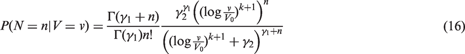
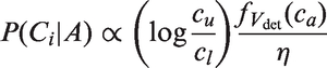
The likelihoods described in equations (18) and (19) are the joint probabilities of tumours belonging to size interval i and having j affected lymph nodes, conditioned on mode of detection, numbers and times of previous negative screens, and mammographic density (the latter is omitted from the likelihood expressions for simplicity, but is included in our calculations for the analyses presented in the next section). There are seven different quantities in the likelihood, which we express in terms of models (3) to (5), the screening sensitivity (17), and lymph node models (7) and (8), (10) and (11), (12) and (13), or (15) and (16).

The first quantity is $P (B_{0} | C_{i})$ , the probability for a positive screen, given the size of the tumour. This is the screening sensitivity, which we model using equation (17). This quantity helps adjust the tumour size distribution of screened tumours, which is different from the tumour size distribution of symptomatic tumours.

The second quantity is $P (C_{i} | D)$ , the probability of being in size interval i, given symptomatic detection, which is equal to $\frac{P (C_{i}, D)}{P (D)}$ . Without further information, P(D) is constant, and thus the $P (C_{i} | D)$ is equal to the probability of having a symptomatic detection at size interval i. Based on equations (1), (4), and (5), Plevritis et al.⁷ showed that the volume at symptomatic detection $V_{det}$ is given by

f_{V_{det}} (v) = η τ_{1} \frac{τ_{2}^{τ_{1}}}{{(τ_{2} + η (v - V_{0}))}^{τ_{1} + 1}}, v \geq V_{0}

(20)

The proof is based on integrating (5) from V₀ to infinity. Since our value of V₀ is the same as in Plevritis, and the tumour starts growing before this value, we can use equation (20) to calculate

P (C_{i} | D)

. It should be noted that this factor only conditions on the tumour being symptomatic. In other words, this factor does not take into consideration that there have been previous negative screens. This is instead accounted for by quantities five and seven.

The third quantity is $P (C_{i} | A)$ , the probability that the tumour is in size interval i, given that there is a clinically detectable tumour in the breast. Isheden and Humphreys¹⁰ showed that this quantity satisfies

\begin{matrix} P (C_{i} | A) \propto (log \frac{c_{u}}{c_{l}}) \frac{f_{V_{det}} (c_{a})}{η} \end{matrix}

where

c_{u} / c_{l}

is the upper/lower bound of tumour size interval i, and c_a is some average value between c_u and c_l. We calculate this quantity with c_a being the geometric mean of c_u and c_l. As with quantity two, this quantity does not take into consideration previous negative screens or the current positive screen. Those factors are instead adjusted for by quantities one, five, and six.

The fourth quantity is $P (N_{j} | C_{i})$ , the probability of having j lymph nodes affected when the tumour is in size interval i. To calculate this probability we use equation (8) in model A, we use equation (11) in model B, we use equation (13), for the class of lymph spread models, and we use equation (16) for the random effects model. These equations are conditioning on a single value of the volume. For approximating the probability when conditioning on a tumour size interval, our conditioning value is the geometric mean of the upper and lower bounds of size interval i. This factor describes only the number of lymph nodes conditional on tumour size interval. The screening history is adjusted for by quantities one, five, six, and seven.

The fifth quantity is $P (B^{c} | C_{q, t_{1}} \cap C_{i})$ , the probability of n negative previous screens, given the size of the tumour at the first previous negative screen and the size at detection. This probability is calculated as

P (B^{c} | C_{q, t_{1}} \cap C_{i}) = P (B_{1}^{c}) \cdot P (B_{2}^{c}) \cdot \dots \cdot P (B_{n}^{c})

where

P (B_{m}^{c})

is the probability of a negative screening at the mth screen prior to detection, calculated from equation (17). The sizes of the tumour at the previous screens are calculated by projecting backwards from the trajectory intersecting the midpoints of intervals q and i. This is one of four quantities that adjust for the screening history in the likelihood.

The sixth quantity is $P (C_{q, t_{1}} | C_{i} \cap N_{j})$ , the probability to be in size interval q at time point t₁, given that the tumour is found in size interval i with j lymph nodes affected. It is calculated by marginalising the probability over growth rate, using

P (C_{q, t_{1}} | C_{i} \cap N_{j}) = \int_{r = 0}^{\infty} P (C_{q, t_{1}} | C_{i} \cap N_{j} \cap (R = r)) f_{R | C_{i} \cap N_{j}} (r) d r

We approximate

P (C_{q, t_{1}} | C_{i} \cap N_{j} \cap (R = r))

by 1 if a tumour in size interval i, growing with an inverse growth rate r, passes the q:th size interval t₁ years previous to detection, and 0 otherwise. For models A and B and for the class of lymph spread models, it holds that

\begin{matrix} f_{R | C_{i} \cap N_{j}} (r) \approx f_{R | V_{\det} = v} (r) = \frac{(τ_{2} + η (v - V_{Cell}))}{Γ (τ_{1} + 1)} (r (τ_{2} + η (v - V_{Cell})))^{(τ_{1} + 1) - 1} exp (- r (τ_{2} + η (v - V_{Cell}))), r \geq 0 \end{matrix}

where v is the geometric mean of the upper and lower bounds of size interval i. In all three cases, this follows from the fact that

\frac{f_{R | C_{i} \cap N_{j}} (r)}{f_{R | C_{i}} (r)} = \frac{P (N = j | R = r \cap C_{i})}{P (N = j | C_{i})} = 1 \Rightarrow f_{R | C_{i} \cap N_{j}} (r) = f_{R | C_{i}} (r)

and from Theorem 3 in Isheden and Humphreys,¹⁰ which states that

\begin{matrix} f_{R | C_{i}} (r) \approx f_{R | V_{\det} = v} (r) \\ = \frac{(τ_{2} + η (v - V_{Cell}))}{Γ (τ_{1} + 1)} (r (τ_{2} + η (v - V_{Cell})))^{(τ_{1} + 1) - 1} exp (- r (τ_{2} + η (v - V_{Cell}))), r \geq 0 \end{matrix}

This quantity accounts for the tumour growth rate when adjusting for the screening history in the likelihood for screen detected tumours.

The seventh quantity is $P (C_{q, t_{1}} | C_{i} \cap N_{j} \cap D)$ , the probability to be in size interval q at time point t₁, given that the tumour is symptomatically detected in size interval i with j lymph nodes affected. This quantity is calculated in the same way as the sixth quantity. This quantity accounts for the tumour growth rate when adjusting for the screening history in the likelihood for symptomatic tumours.

For the four lymph node spread models described here, the likelihood is separable; we can separate into a size component and a nodes component. This can be seen, for example for the likelihood for screening cases, by writing

\begin{matrix} P (C_{i} \cap N_{j} | A \cap B_{0} \cap B^{c}) = p_{i, j} \\ \propto P (N_{j} | C_{i}) P (B_{0} | C_{i}) P (C_{i} | A) (\sum_{q \leq i} P (B^{c} | C_{q, t_{1}} \cap C_{i}) P (C_{q, t_{1}} | C_{i} \cap N_{j})) \\ = P (N_{j} | C_{i}) P (B_{0} | C_{i}) P (C_{i} | A) (\sum_{q \leq i} P (B^{c} | C_{q, t_{1}} \cap C_{i}) P (C_{q, t_{1}} | C_{i})) \\ \propto P (N_{j} | C_{i}) P (C_{i} | A \cap B_{0} \cap B^{c}) \end{matrix}

The same goes for the likelihood for symptomatic cases.

For the models of Hanin and Yakovlev¹⁴ and Shwartz,¹³ the likelihood calculation is not as straightforward. The quantity $P (C_{q, t_{1}} | C_{i} \cap N_{j})$ has to be calculated by marginalising over growth rate using $F_{R | V = v, N_{j} = n} (r)$ . In both cases, $F_{R | V = v, N_{j} = n} (r) \neq F_{R | V = v} (r)$ , which means that the likelihood does not separate into two components which can be optimised independently. For example, for Hanin and Yakovlev's lymph node spread model, i.e. with $λ (t) = σ V (t)$ , it can be shown that

F_{R | V = v, N_{j} = n} (r) = \frac{γ (τ_{1} + 1 + n, r (τ_{2} + η (v - v_{0}) + σ (v - v_{0})))}{Γ (τ_{1} + 1 + n)}

For their lymph node spread model

P (N_{j} | C_{i})

is calculated using

P (N_{j} = n | V_{\det} = v) = \frac{Γ (n + τ_{1} + 1)}{Γ (τ_{1} + 1) n!} \frac{{(σ (v - v_{0}))}^{n} {(τ_{0} + η (v - v_{0}))}^{τ_{1} + 1}}{{(σ (v - v_{0}) + τ_{2} + η (v - v_{0}))}^{n + τ_{1} + 1}}

The likelihood that we describe in this section is complex. It relies on several approximations that are needed mainly to account for discretisation in the estimation procedure. To verify that we implemented the methods correctly, we performed a simulation study. The aim of the study was to show that we can accurately retrieve parameter estimates from the likelihood. The results are shown in Appendix 1.

5 Joint modelling of tumour size and lymph node spread – a study of incident invasive breast cancer in post-menopausal women

We illustrate the joint approach by fitting models A and B to 1860 cases of incident invasive breast cancer from a case-control study of post-menopausal breast cancer¹⁸ known as CAHRES. The study invited all Swedish born women ages 50–74 that were diagnosed with invasive breast cancer in Sweden from October 1993 to March 1995. The participation rate of the study was 84% (n = 3345). In extensions of the study, analog mammographic images were retrieved from mammography screening units and radiology departments managing mammography screening in Sweden. Information on tumour size, screening history, and mode of detection was collected from the Swedish Cancer Registry and the Stockholm-Gotland Breast Cancer Registry. The collection of this data has been described previously by Rosenberg et al.^19,20 and Eriksson et al.²¹ We excluded women from our analysis if they had missing lymph node status, lacked written consent, had a previous or other cancer diagnosis, had a noninvasive breast cancer diagnosis, were diagnosed before or after study period, were pre-menopausal, had unknown age at menopause, lacked screening information, lacked images, had a missing mode of diagnosis, or were missing tumour size. After those exclusions, 1860 were cases available for analysis. Descriptive information on the 1860 cases included in our analyses is presented in Table 1.

Table 1.

Comparison of screening and symptomatically detected cancers in CAHRES.

	Screening	Symptomatic
Number of cases	1133	727
Tumour size in mm (median and quartiles)	$12 (9, 18)$	20 (13, 26)
Percentage density (median and quartiles)	$13.6 (6.8, 23.3)$	$15.7 (8.6, 28.1)$
Time since last negative screen in years^a (median and quartile)	$2.0 (1.8, 2.1)$	$1.4 (1.0, 2.0)$
Number of previous screens
Cases with no previous screen	133	197
Cases with one previous screen	214	105
Cases with two previous screens	658	247
Cases with three or more previous screens	128	178
Number of affected lymph nodes
Cases with no affected lymph nodes	890	438
Cases with one affected lymph node	103	104
Cases with two affected lymph nodes	45	55
Cases with three or more affected lymph nodes	95	130

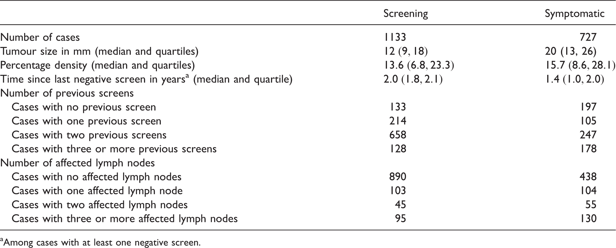
Among cases with at least one negative screen.

We fitted model A and model B by maximising the likelihood over parameters $τ_{1},$ $τ_{2},$ $η,$ $β_{1},$ $β_{2}$ , $β_{3},$ and σ_A or σ_B. Parameter estimates are given in Table 2. For each model, we used 200 non-parametric bootstrap replicates to estimate 95% coverage intervals, using the percentile method. Comparing the two models in terms of their likelihood values, it is clear that model B provides a much better fit to the data than model A. Model-based estimates of expected lymph node spread as a function of tumour size are plotted alongside observed numbers in Figure 1 (neither model fits the data well). In the figure, each circle represents the observed averages for each tumour size interval. The bars intersecting each circle represent 95% confidence intervals, obtained via bootstrapping.

Figure 1.

Model-based estimates of expected lymph node spread as a function of tumour size, based on CAHRES. Circles and bars represent averages and 95% confidence intervals of numbers of lymph nodes affected within each tumour size interval. Model A (dotted) produces excessive spread at large tumour sizes, while model B (solid) underestimates spread at large tumour sizes.

Table 2.

Parameter estimates in joint models of tumour size and lymph node spread, together with bootstrapped 95% coverage intervals, based on 1860 post-menopausal breast cancer cases (CAHRES).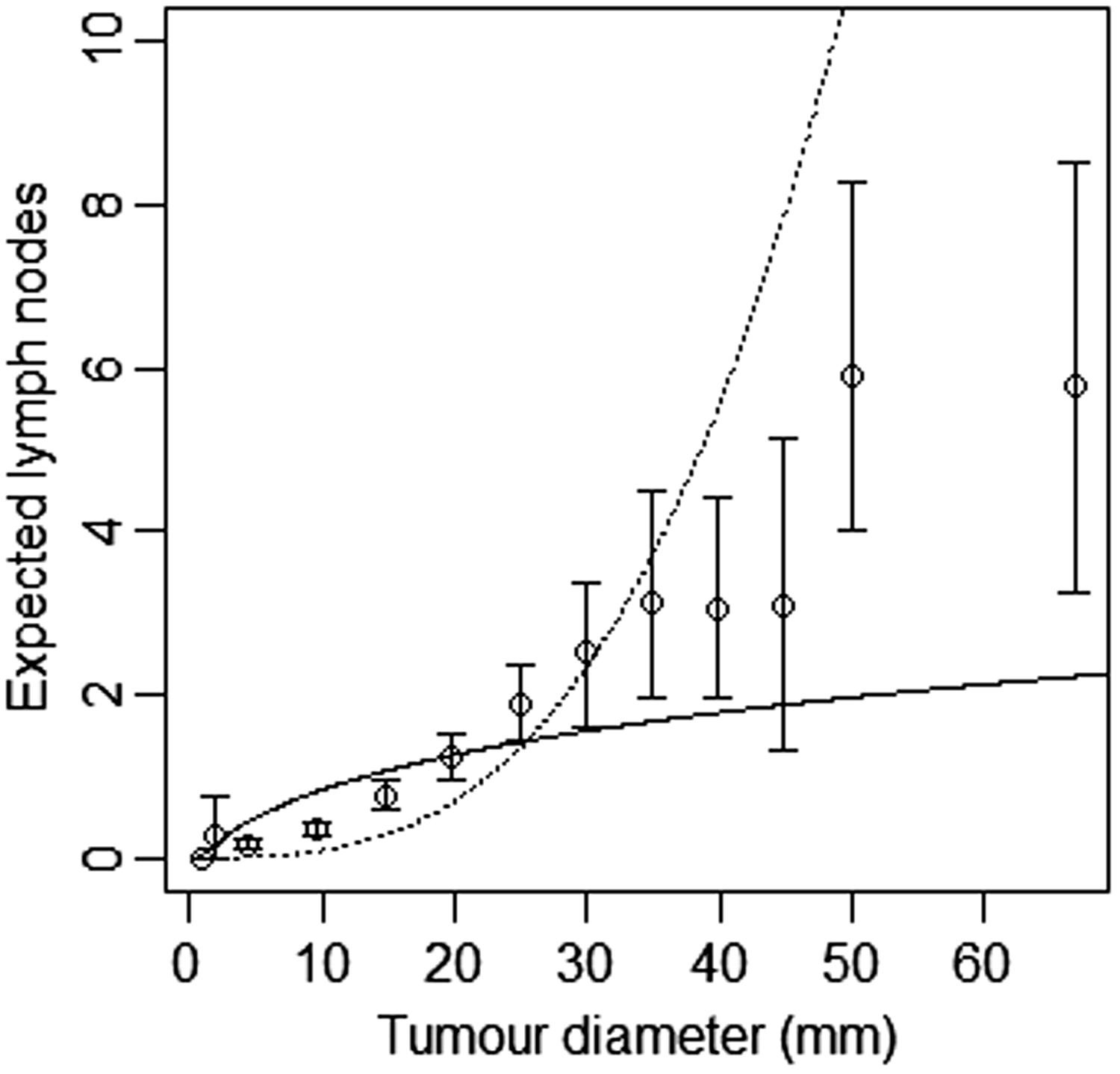

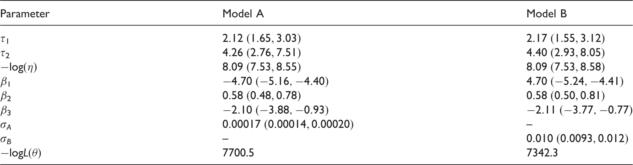
Parameter	Model A	Model B
τ ₁	$2.12 (1.65, 3.03)$	$2.17 (1.55, 3.12)$
τ ₂	$4.26 (2.76, 7.51)$	$4.40 (2.93, 8.05)$
$- log (η)$	$8.09 (7.53, 8.55)$	$8.09 (7.53, 8.58)$
β ₁	$- 4.70 (- 5.16, - 4.40)$	$4.70 (- 5.24, - 4.41)$
β ₂	$0.58 (0.48, 0.78)$	$0.58 (0.50, 0.81)$
β ₃	$- 2.10 (- 3.88, - 0.93)$	$- 2.11 (- 3.77, - 0.77)$
σ _A	$0.00017 (0.00014, 0.00020)$	–
σ _B	–	$0.010 (0.0093, 0.012)$
$- log L (θ)$	7700.5	7342.3

We attempted to jointly fit the tumour growth model with the lymph spread models of Hanin and Yakovlev, and Shwartz. In both cases, the models did not converge, and we were not able to retrieve parameter estimates. Their lymph spread models are not consistent with the data (see Section 2). If we would have been able to get the joint model to converge, we know that the lymph node models of Hanin and Yakovlev and Shwartz would have over-estimated the number of affected lymph nodes at large tumour sizes and underestimated the number of affected lymph nodes at small tumour sizes to the same extent as model A does. Although model B does underestimate the number of lymph nodes at larger tumour sizes, overall, it provides a better fit to the data than model A, and the models of Hanin and Yakovlev, and Shwartz.

Next, we experimented with other functional forms from our new class of lymph node spread models. In Table 3, we display estimates of the parameter σ from equations (12) and (13) for

k = 1, 2, 3, 4, 5, 6

, together with optimised log-likelihood values from fitting the joint models of tumour size and spread to the 1860 breast cancer cases.

Table 3.

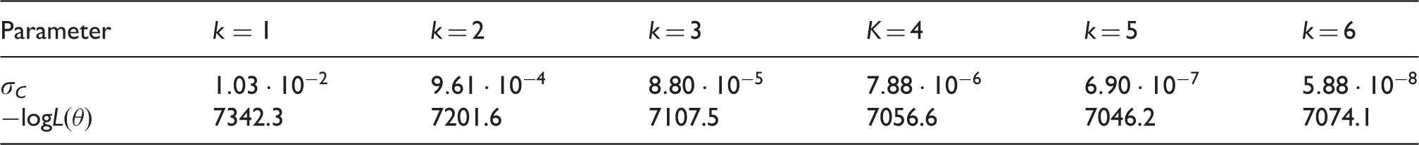
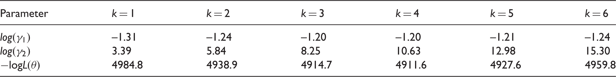
Parameter estimates and log-likelihood values for different functional forms of the Poisson lymph node spread model (CAHRES).

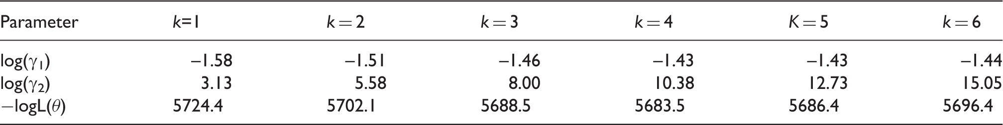
Parameter	$k = 1$	k = 2	k = 3	K = 4	k = 5	k = 6
σ _C	$1.03 \cdot 10^{- 2}$	$9.61 \cdot 10^{- 4}$	$8.80 \cdot 10^{- 5}$	$7.88 \cdot 10^{- 6}$	$6.90 \cdot 10^{- 7}$	$5.88 \cdot 10^{- 8}$
$- log L (θ)$	7342.3	7201.6	7107.5	7056.6	7046.2	7074.1

Table 4.

Parameter estimates and log-likelihood values for different functional forms of the random effects lymph node spread model (CAHRES).

Parameter	k=1	k = 2	k = 3	k = 4	K = 5	k = 6
log(γ₁)	–1.58	–1.51	–1.46	–1.43	–1.43	–1.44
log(γ₂)	3.13	5.58	8.00	10.38	12.73	15.05
−logL(θ)	5724.4	5702.1	5688.5	5683.5	5686.4	5696.4

From the integer values, we achieved the best model fit for k = 5, with a log-likelihood difference of 296.1 compared to the spread component of model B (k = 1). Varying both σ_C and k, we found the optimal value of k to be 4.75, with 95% confidence interval $(4.47, 5.05)$ , based on the profile likelihood. In Figure 2, we plot estimates of expected lymph node spread based on the model with k = 5, alongside those based on model A.

Figure 2.

Model-based estimates of expected lymph node spread as a function of tumour size (CAHRES). Circles and bars represent averages and 95% confidence intervals of numbers of lymph nodes affected within each tumour size interval. The spread component of Model A (dotted) produces excessive spread in large tumours, whereas in terms of expected numbers of affected lymph nodes the spread model with k = 5 (solid) fits at all tumour sizes.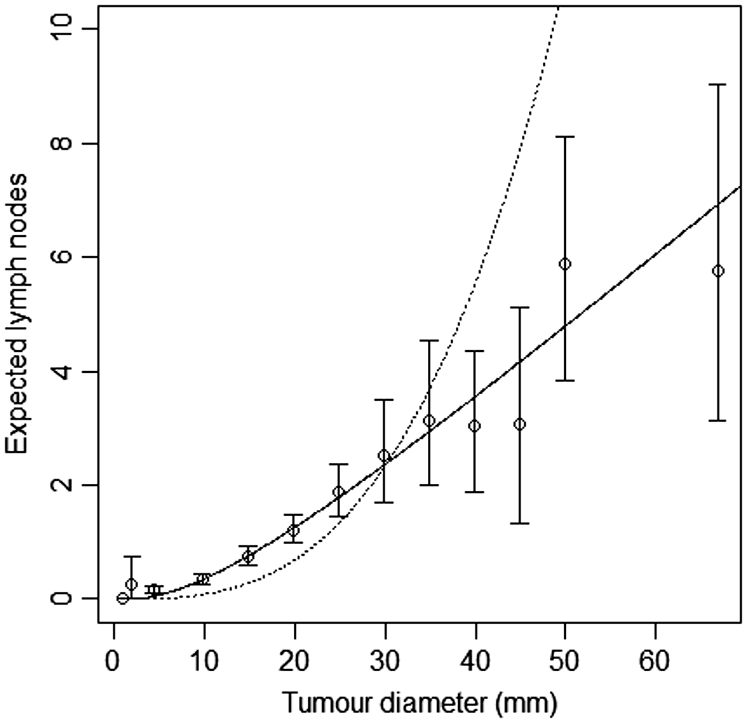

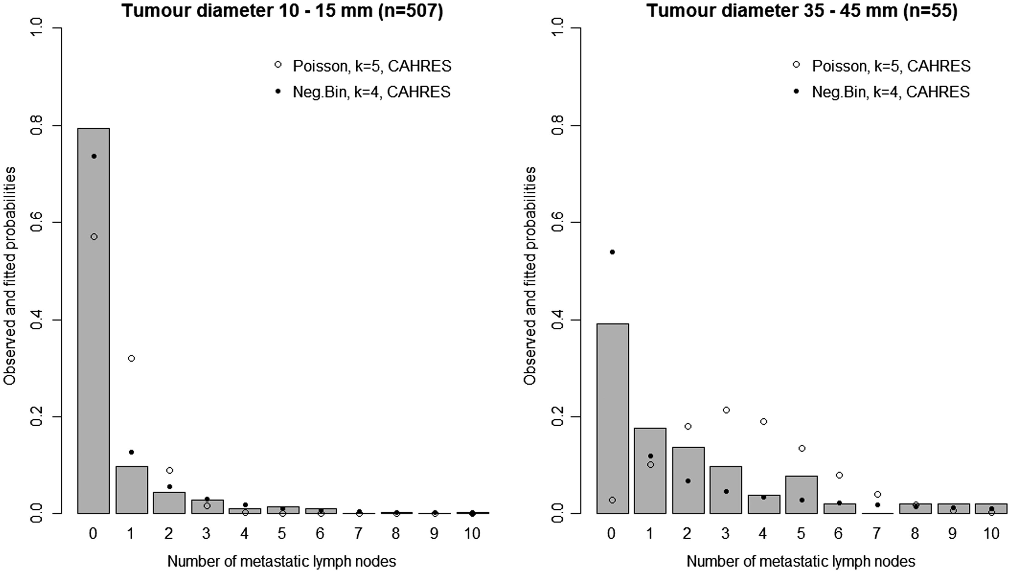
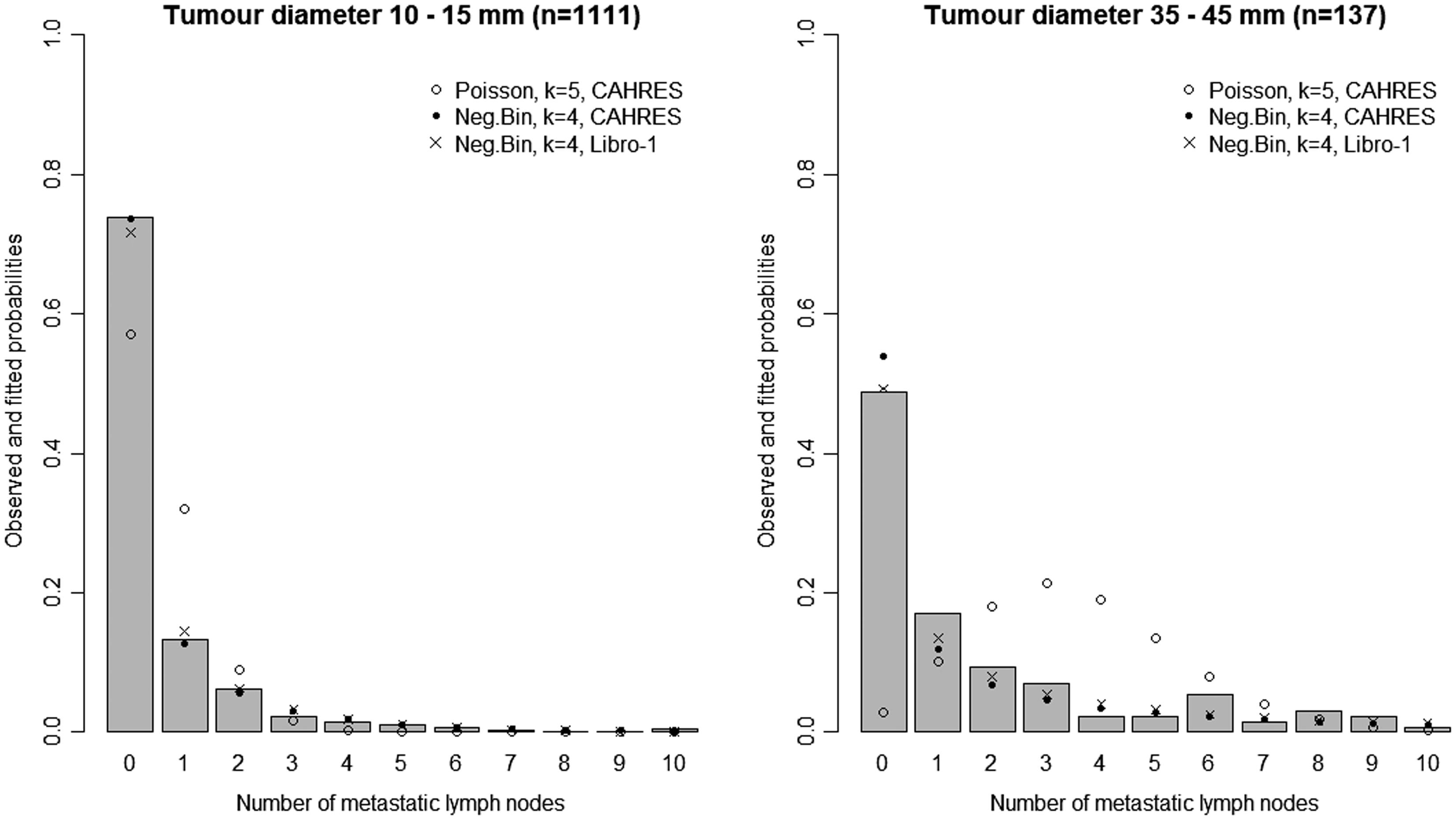
We fitted joint models of tumour size and lymph node spread, based on the random effects models described by equations (15) and (16), for $k = 1, 2, 3, 4, 5, 6$ ; see Table 4. Allowing for heterogeneity in rates of spread improved model fit tremendously for all considered integer values of k. Improvements in optimised log-likelihood values ranged from 1617.9 to 1359.8, and differences in model fit, across different values of k, also diminished greatly. Varying $γ_{1}, γ_{2},$ and k, we obtained an estimate of 4.11 for k, with a 95% confidence interval $(3.44, 4.75)$ .

In Figure 3, we plot estimates of expected number of lymph nodes affected based on the random effects lymph spread model with k = 4. These estimates pass through all the 95% confidence intervals (except one, which comes very close). In Figure 4 we plot the observed numbers of lymph nodes (bars) within two size categories, along with the model predicted probabilities at the end points of the intervals. The random effects model accounts for overdispersion in relation to the Poisson model. We note that if we were to represent model A, allowing or not allowing for overdispersion, even in this plot, the prediction of the mean value of the number of lymph nodes would be overestimated for large tumour sizes.

Figure 3.

Model-based estimates of expected lymph node spread as a function of tumour size (CAHRES). Circles and bars represent averages and 95% confidence intervals of numbers of lymph nodes affected within each tumour size interval. The spread component of Model A (dotted) is plotted alongside the random effects spread model with k = 4 (solid).

Figure 4.

Observed and predicted numbers of affected lymph nodes (CAHRES). The bars represent the observed numbers of affected lymph nodes, within tumour size interval 10–15 mm (left) and 35–45 mm (right), in the CAHRES dataset. Circles represent predicted probabilities from the Poisson model with k = 5, estimated on the CAHRES data set, and dots represent predicted probabilities from the random effects Poisson model with k = 4, also estimated on the CAHRES data set.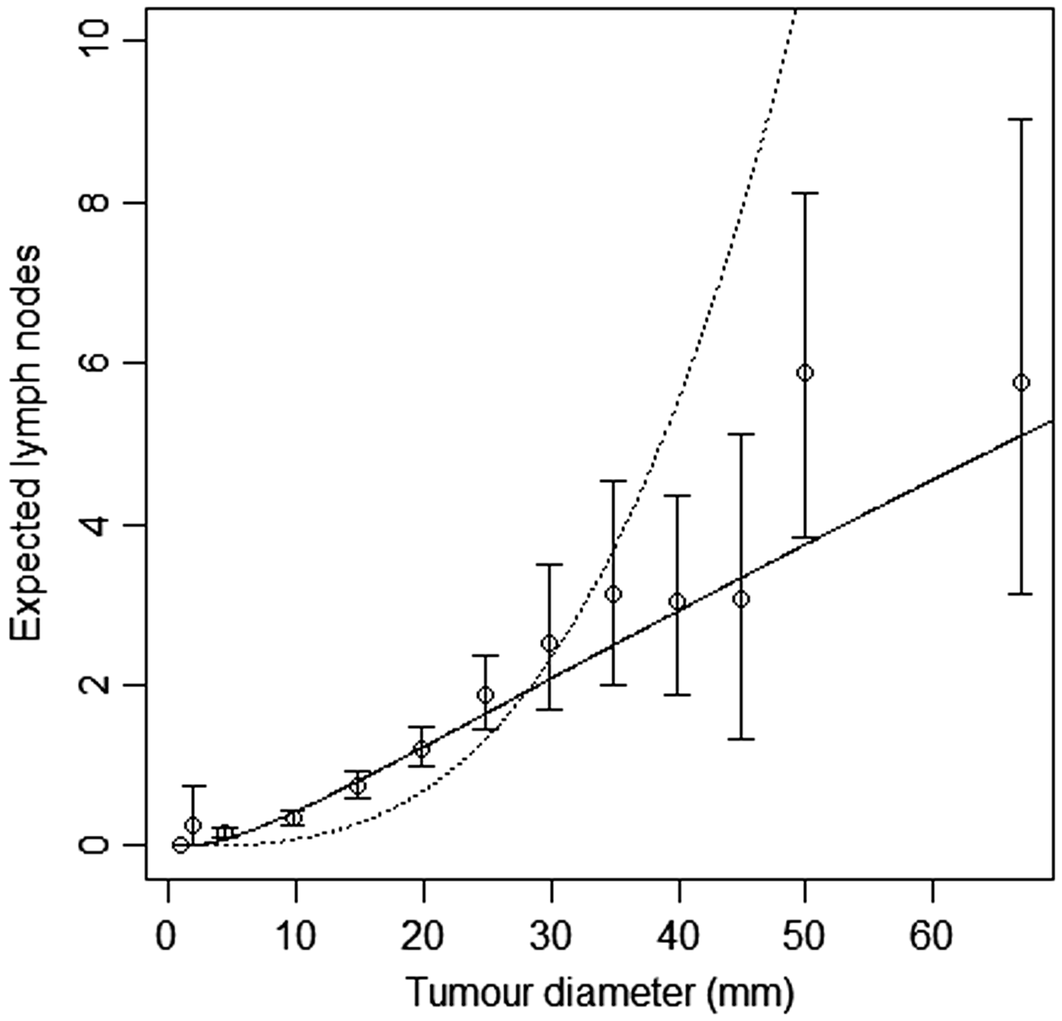

Finally for CAHRES, we divided the data set into screen detected cases and symptomatically detected cases, and plotted 95% confidence intervals for average number of affected lymph nodes, along with the model-based estimates obtained from fitting model A and the random effects Poisson model with k = 4; see Figure 5. Although the estimates based on our selected model intersect all but one of the confidence intervals, there is some suggestion (at large tumour sizes) that the model could be underestimating expected number of lymph nodes in symptomatic cases and overestimating the expected numbers in screening cases.

Figure 5.

Model-based estimates of expected lymph node spread as a function of tumour size (CAHRES). To the left, circles and bars represent averages and 95% confidence intervals of numbers of lymph nodes affected within each tumour size interval for screen detected cancers, and to the right the corresponding quantities for symptomatically detected cancers. On both figures, the spread component of Model A (dotted) is plotted alongside the random effects spread model with k = 4 (solid).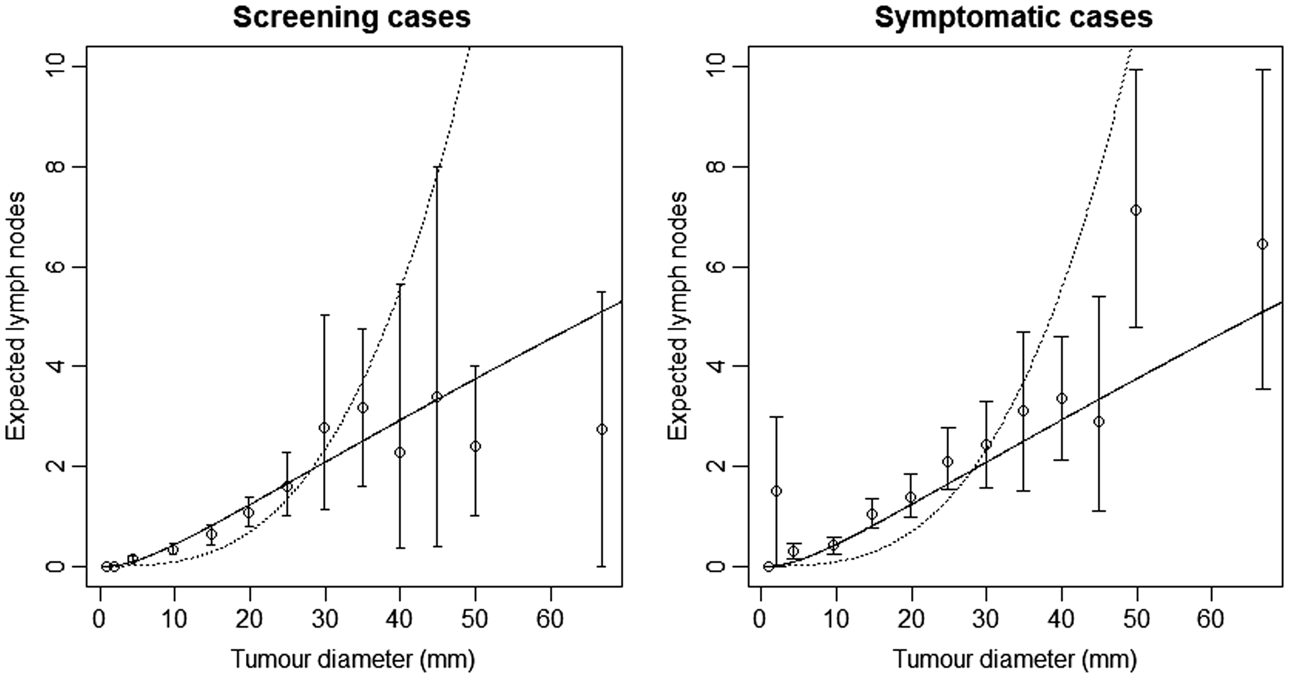

6 Validation study of the random effects lymph node spread model

We attempted to validate our lymph node spread model using an independent data set of women diagnosed with invasive breast cancer between January 1, 2001 and December 31, 2008 in the Stockholm-Gotland healthcare region in Sweden, known as Libro-1. These women were identified though the Regional Breast Cancer Register. Information on diagnosis and tumour characteristics were available, but not on time and number of screening rounds. Women were excluded if they were less than 50 years old, underwent diagnostic operations, were pre-operatively diagnosed with in situ breast cancer but pathology reports showed an invasive component, had incorrect dates of diagnosis, had more than 63 days between diagnosis and date of surgery, had missing tumour size, or missing lymph node status. In 2007, the registers changed the definitions and procedures for evaluating lymph node spread. To keep the data set comparable to the CAHRES data set, we excluded women that were categorised according to the new standard. The final data set consisted of 3961 women.

In Figure 6, we plot 95% confidence intervals of number of affected lymph nodes, within tumour size intervals, based on the Libro-1 data (bars), along with the expected number of lymph nodes, as a function of tumour diameter, based on the random effects model with k = 4, estimated from the CAHRES data. We also fitted the random effects model to the Libro-1 data with $k = 1, 2, 3, 4, 5, 6$ ; see Table 5. With an integer value for k, model fit was best at k = 4 also on this data set. Estimates of expected numbers of affected lymph nodes for this model are plotted as the solid line in Figure 6. In Figure 7, we plot the observed numbers of lymph nodes (bars) within two size categories, for the Libro-1 data, along with the model predicted probabilities at the end points of the intervals (i.e. self-trained), based on the random effects models fitted to CAHRES data, and Libro-1 data, and also the Poisson model with k = 5, estimated from CAHRES without random effects. Even with parameter values obtained from the CAHRES data, the random effects (k = 4) lymph node spread model seems to fit the Libro-1 data on numbers of affected lymph nodes extremely well.

Figure 6.

Model-based estimates of expected lymph node spread as a function of tumour size based on the random effects Poisson model (k = 4), estimated on CAHRES (dotted line) and Libro-1 (solid line), along with 95% confidence intervals of average lymph node spread obtained from Libro-1.

Figure 7.

Observed and predicted numbers of affected lymph nodes (Libro-1). The bars represent the observed numbers of affected lymph nodes, within tumour size interval 10–15 mm (left) and 35–45 mm (right), in the Libro-1 dataset. Circles represent predicted probabilities from the Poisson model with k = 5, estimated on the CAHRES data set, dots represent predicted probabilities from the random effects Poisson model with k = 4, also estimated on the CAHRES data set, and crosses represent estimated probabilities from the random effects Poisson model with k = 4, estimated on the Libro-1 data set.

Table 5.

Parameter estimates and log-likelihood values for different functional forms of the random effects lymph node spread model (Libro-1).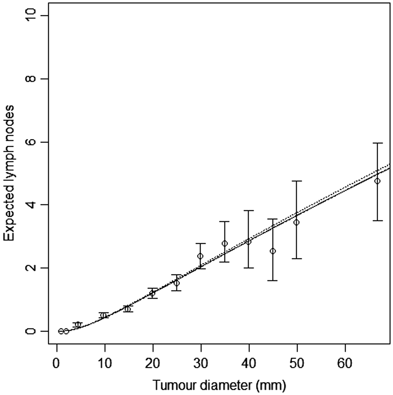

Parameter	k = 1	k = 2	k = 3	k = 4	k = 5	k = 6
$log (γ_{1})$	–1.31	–1.24	–1.20	–1.20	–1.21	–1.24
$log (γ_{2})$	3.39	5.84	8.25	10.63	12.98	15.30
$- log L (θ)$	4984.8	4938.9	4914.7	4911.6	4927.6	4959.8

When estimating $γ_{1}, γ_{2},$ and k from the Libro-1 data, we estimated k to have a value of 3.65 and a 95% confidence interval of $(3.22, 4.05)$ . 95% confidence intervals for k, estimated from Libro-1 and CAHRES, overlapped, and both included k = 4.

7 Discussion

Continuous growth models offer an interesting alternative to multi-state Markov models for studying the natural history of breast cancer. Previously proposed continuous growth models have components for tumour growth, time to symptomatic detection, and screening sensitivity. The aim of this article has been to add an additional component for lymph node spread. We began this article by reviewing the literature of breast cancer lymph spread models. We identified two models, one from Hanin and Yakovlev,¹⁴ and one from Shwartz,¹³ which is also used by the CISNET University of Wisconsin group. Both models are Poisson processes with intensity functions dependent on tumour volume. In this paper, we show that these models have two weaknesses. The first is that slow growing tumours spread more quickly than fast growing tumours, and the second is that the rate of additional lymph node spread grows excessively with increasing tumour volume. In order to avoid these two weaknesses, we have improved upon the existing models and developed new models of lymph node spread in a step-by-step fashion. We focused first on modelling the mean structure and then extended the lymph node spread model to incorporate random effects.

The first step of the process was to construct a model A, which avoids an inverse relation between tumour growth rate and lymph node spread. This was done by removing the terms from the intensity function that contributed to the inverse relationship in Shwartz¹³ model. We were able to estimate the parameters of model A jointly with the tumour growth models (see Table 2). This was not the case with the models of Hanin and Yakovlev,¹⁴ or Shwartz. Since we were not able to make those models converge and since we were able to remove the inverse relationship between tumour growth rate and lymph node spread, we consider model A an improvement on Hanin and Yakovlev, and Shwartz.

In the second step, we created model B. At this step, we addressed the second weakness. Model A assumes a linear relationship between the expected number of lymph nodes affected and tumour volume. Because tumour growth is assumed to be exponential with time, this linear relationship implies that the number of affected lymph nodes grows exponentially with time. To decrease the rate of spread in the model, we introduce a logarithmic term. We assume that the intensity function depends on the number of cell divisions instead, which is equivalent to the tumour volume divided by the volume of a single cell. We found that model B was an improvement on model A, although it overestimated spread at small tumour sizes and underestimated spread at large tumour sizes.

Model B removes the exponential spread behaviour of previous models in the literature, and provides a basis on which to build further. We tested different shapes of the spread functions by introducing a class of lymph spread models. These models differ in their shape, defined by a factor k, with model B represented as a special case (k = 1). In this model class, we found that k = 5 provided good model fit. In terms of expected values, this model fitted well across all tumour volumes. By extending the lymph node spread models to allow for random effects, we were able to incorporate heterogeneity in rates of lymph node spread. This extension turned out to be extremely important, and corrected for overdispersion with respect to the classical Poisson models. In fitting the overdispersed random effects model, we obtained a point estimate of k = 4.11 using the CAHRES study data, and an estimate of k = 3.65 using the Libro-1 study data. The 95% confidence intervals for k, estimated on the two data sets, overlapped and included k = 4; this value provided good model fit in both data sets.

The analyses in this paper rely on the assumptions of a stable disease population and the assumption that screening attendance is independent of tumour growth rate. For the joint analysis of size and lymph node spread, we have worked with CAHRES, a nationwide cohort with 84% participation rate. The study invited all Swedish born women ages 50 to 74 that were diagnosed with invasive breast cancer in Sweden from October 1993 to March 1995. In the absence of screening, a population satisfying stable disease assumptions will exhibit a constant incidence of breast cancer.¹⁰ Once a screening program has run for a number of years, we expect a constant incidence if the stable disease assumptions hold. Of the 26 counties in Sweden, 22 had implemented screening programmes by, and in many cases well before, 1990,²² and incidence data from the Swedish Cancer Registry shows that breast cancer incidence was approximately constant between 1991 and 1997.²³ In the current study, all women were post-menopausal at diagnosis. It is unlikely that a large fraction of the women took part in extra surveillance for breast cancer, which means that the assumption that screening attendance is independent of tumour growth rate is likely to be reasonable.

The joint model of tumour growth and lymph node spread has two main areas of application. The first one is for evaluating screening programs, which can be done via microsimulation. Several research groups^12,24 have used Markov models to simulate the natural history of breast cancer. As the number of disease states increases, these models become impractical, especially if the objective is to simulate screening options based on individual risk factors. For this, continuous growth models present a strong alternative. The second area of application is to study factors behind growth and spread. Abrahamsson et al.¹¹ used continuous growth models to regress BMI on the log inverse growth rate, and breast size on the log of the hazard proportionality constant in the model for time to symptomatic detection, and Isheden and Humphreys¹⁰ studied in detail the relationship between mammographic density, tumour size, and screening sensitivity. For the new sub-model for lymph node spread, we are currently working on extensions of the model to study association with observable factors, both traditional breast cancer risk factors and tumour characteristics/subtypes.

As we have pointed out, our models assume several well known biological properties of cancer. The fact, however, that the k = 4 model fits better than the k = 1 model implies that there may be a degree of genomic instability as breast cancer cells divide. Finally, we point out that in our work we have not been able to specify a tractable model where fast growing tumours spread more rapidly than slow growing ones. It is possible that an alternative model with this characteristic will also provide a good fit to incidence data on tumour size and lymph node spread.

Footnotes

Acknowledgements

We are grateful to Wei He for assisting in data retrieval, to Mark Clements, Alexander Ploner, and Ola Hössjer for valuable discussions.

Declaration of conflicting interests

The author(s) declared no potential conflicts of interest with respect to the research, authorship, and/or publication of this article.

Funding

The author(s) disclosed receipt of the following financial support for the research, authorship, and/or publication of this article: This work was supported by the Swedish Research Council (2016-01245), the Swedish Cancer Society (CAN 2017/287) and the Swedish e-Science Research Centre.

References

Duffy

Chen

Tabar

, et al. Estimation of mean sojourn time in breast cancer screening using a Markov chain model of both entry to and exit from the preclinical detectable phase. Stat Med 1995; 14: 1531–1543.

Chen

Duffy

Day

. Markov chain models for progression of breast cancer. Part I: tumour attributes and the preclinical screen-detectable phase. J Epidemiol Biostat 1997; 2: 9–23. .

Chen

Duffy

Tabar

, et al. Markov chain models for progression of breast cancer. Part II: prediction of outcomes for different screening regimes. J Epidemiol Biostatist 1997; 2: 25–35. .

Uhry

Hédelin

Colonna

, et al. Multi-state Markov models in cancer screening evaluation: a brief review and case study. Stat Meth Med Res 2010; 19: 463–486.

Weedon-Fekjær

Tretli

Aalen

. Estimating screening test sensitivity and tumour progression using tumour size and time since previous screening. Stat Meth Med Res 2010; 19: 507–527.

Bartoszyński

Edler

Hanin

, et al. Modeling cancer detection: tumor size as a source of information on unobservable stages of carcinogenesis. Math Biosci 2001; 171: 113–142.

Plevritis

Salzman

Sigal

, et al. A natural history model of stage progression applied to breast cancer. Stat Med 2007; 26: 581–595.

Weedon-Fekjær

Lindqvist

Vatten

, et al. Breast cancer tumor growth estimated through mammography screening data. Breast Cancer Res 2008; 10: R41.

Abrahamsson

Humphreys

. A statistical model of breast cancer tumour growth with estimation of screening sensitivity as a function of mammographic density. Stat Meth Med Res 2016; 25: 1620–1637.

10.

Isheden

Humphreys

. Modelling breast cancer tumour growth for a stable disease population. Stat Meth Med Res 2017, pp. 0962280217734583..

11.

Abrahamsson

Czene

Hall

, et al. Breast cancer tumour growth modelling for studying the association of body size with tumour growth rate and symptomatic detection using case-control data. Breast Cancer Res 2015; 17: 1–11.

12.

Berry

Cronin

Plevritis

, et al. Effect of screening and adjuvant therapy on mortality from breast cancer. New Engl J Med 2005; 353: 1784–1792.

13.

Shwartz

. An analysis of the benefits of serial screening for breast cancer based upon a mathematical model of the disease. Cancer 1978; 41: 1550–1564.

14.

Hanin

Yakovlev

. Multivariate distributions of clinical covariates at the time of cancer detection. Stat Meth Med Res 2004; 13: 457–489.

15.

Schwartz

. A biomathematical approach to clinical tumor growth. Cancer 1961; 14: 1272–1294.

16.

Toi

Taniguchi

Ueno

, et al. Significance of circulating hepatocyte growth factor level as a prognostic indicator in primary breast cancer. Clin Cancer Res 1998; 4: 659–664.

17.

Hanahan

Weinberg

. Hallmarks of cancer: the next generation. Cell 2011; 144: 646–674.

18.

Magnusson

Baron

Persson

, et al. Body size in different periods of life and breast cancer risk in post-menopausal women. Int J Cancer 1998; 76: 29–34.

19.

Rosenberg

Magnusson

Lindström

, et al. Menopausal hormone therapy and other breast cancer risk factors in relation to the risk of different histological subtypes of breast cancer: a case-control study. Breast Cancer Res 2006; 8: R11.

20.

Rosenberg

Granath

Dickman

, et al. Menopausal hormone therapy in relation to breast cancer characteristics and prognosis: a cohort study. Breast Cancer Res 2008; 10: R78.

21.

Eriksson

Czene

Rosenberg

, et al. The influence of mammographic density on breast tumor characteristics. Breast Cancer Res Treat 2012; 134: 859–866.

22.

Olsson

Andersson

Karlberg

, et al. Implementation of service screening with mammography in Sweden: from pilot study to nationwide programme. J Med Screen 2000; 7: 14–18.

23.

Zahl

Gøtzsche

Mæhlen

. Natural history of breast cancers detected in the Swedish mammography screening programme: a cohort study. Lancet Oncol 2011; 12: 1118–1124.

24.

Chen

Yen

AMF

Tabár

. A stochastic model for calibrating the survival benefit of screen-detected cancers. J Am Stat Assoc 2012; 107: 1339–1359.

25.

Forastero

Zamora

Guirado

, et al. A Monte Carlo tool to simulate breast cancer screening programmes. Phys Med Biol 2010; 55: 5213.

Joint models of tumour size and lymph node spread for incident breast cancer cases in the presence of screening

Abstract

Keywords

1 Introduction

2 Traditional models of regional lymph node spread

3 Joint processes of tumour growth and lymph node spread

3.1 Shared processes and assumptions

3.2 Model A

3.3 Model B

3.4 A new class of models for lymph node spread

3.5 Random effects modelling of lymph node spread

4 Likelihood for incident cases in the presence of screening

4.1 Likelihood for screen detected cases

4.2 Likelihood for symptomatic cases

4.3 Calculating the likelihood

5 Joint modelling of tumour size and lymph node spread – a study of incident invasive breast cancer in post-menopausal women

6 Validation study of the random effects lymph node spread model

7 Discussion

Footnotes

Acknowledgements

Declaration of conflicting interests

Funding

References