A shimming method based on outer mold line control of thin-walled parts

Abstract

Aerospace framework products typically have a thin-walled structure. To ensure the aerodynamic performance of the product, it is necessary to precisely control the shim clearance between the understructure and the skin. However, it is difficult to meet the requirements of product design by digital measurements and calculations of the shim clearance after installing parts on the final assembly or special test stand. To improve the efficiency and accuracy of the shimming process, a method to determine the shimming quantity by a flexible virtual assembly without a physical assembly process is proposed. The proposed method measures the initial shape of the assembly using digital technology that analyzes the assembled shape using a finite element model and calculates the shimming space using the assembled shape. First, the geometric information of the understructure, skin inner mold line (IML), and outer mold line (OML), or the actual pre-assembly shape, are obtained using a three-dimensional laser digitizer. The geometric features are reconstructed and the coordinate transformation matrix is then calculated. The coordinate system is unified based on the positioning features of each part, such as the positioning surface and positioning hole. Finally, the OML of the measured model and the theoretical OML are flexibly fitted to simulate the ideal state of the assembly. The shimming space between the IML and the understructure is calculated and the OML is precisely controlled by shimming. The physical verification results show that the deviation between the analysis results and the actual situation is within 0.1 mm. This method can predict the space of shimming when the OML reaches the ideal state without real assembly thereby reducing the time required for a repeated trial assembly of products and the cost of special measuring tools and conformal tools.

Introduction

The typical structure of aerospace skin components is a framework thin-walled structure. To ensure its aerodynamic performance and streamlined shape, the deviation between the actual outer mold line (OML) and theoretical value must be maintained within a certain range. Because many framework skins have multiple components that affect the understructure, the error accumulation makes difficult to control the OML. The modern aviation industry requires a shimming gap between the assembled metal understructure and the inner mold line (IML) of the matched thin-walled parts. The error of the framework assembly and the processing of the thin-walled part is corrected by the shimming method, which helps control the OML within the required range. This method is time-consuming and prone to quality problems. In addition, the thin-walled parts are easily deformed by the assembly force, which increases the difficulty in determining the space of shimming.

During the assembly of large non-rigid and rigid parts, the specified functional requirements, such as geometric conditions or stresses in joints, should be satisfied. To achieve compliance with the final assembled part, non-compliant operations such as load control, caulking, rigging, or special part manufacturing are required. ¹ Non-rigid parts can be strained by the control force within their stress limits, which results in a slight deformation while eliminating the geometric conditions. These limitations are more stringent for composites. For example, the Airbus A350 XWB is composed of advanced materials (more than 70%), carbon fiber composite materials (53%), titanium, and modern aluminum alloy, which can reduce maintenance requirements and help develop a lightweight and more cost-effective aircraft. ² However, the use of these materials introduces new challenges to manufacturing. To solve the OML deviation caused by the assembly error of large thin-walled parts, it is necessary to add a shim between the understructure and the IML to fill the space between objects. Currently, shimming techniques are widely used in the aerospace industry. Shimming is usually designed into manufacturing schedules to consider the tolerance superposition in the final assembly, so that the OML deviation caused by part manufacturing error and assembly deviation accumulation can be solved effectively. ³

However, the determination of shimming space is a problem that needs to be solved in advance before assembly to save assembly time and improve production efficiency. The purpose of this study is to investigate the OML control of thin-walled parts by means of shimming. In this study, an efficient and automatic shimming method is developed and the feasibility of the method for thin-walled assembly is verified. The measurement method, data processing method, and reconstruction method of the OML, IML, and understructure are determined. Subsequently, an assembly deformation analysis method for thin-walled parts is developed based on the measured model and the shimming method is determined based on the precise control of OML. The advantages of this method are that it can simulate the assembly process and results before the actual assembly which can be used to optimize the assembly process of existing components. Because the manufactured parts remain unchanged and the method of assembling them into their final configuration is optimized, only minor changes in the assembly process may be required.

The remainder of this paper is organized as follows. Section 2 provides an overview of the proposed method. Section 3 presents the definition and mathematical description of the problem. Section 4 describes the methods for measuring and reconstructing the geometric features of the parts. In Section 5, the reconstruction accuracy is analyzed. In Section 6, the assembly feature fitting method is described. Section 7 describes the feasibility analysis of this method through physical verification. The conclusions are presented in Section 8.

Overview

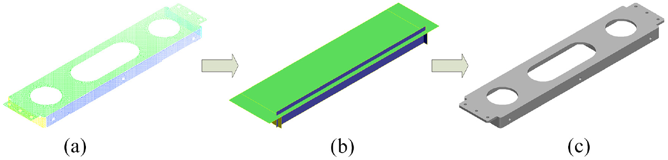
The overall flow of the proposed method is shown in Figure 1. In the first step, a 3D laser scanner is used to obtain the geometric information or the actual pre-assembled shape of the understructure, IML, and OML, and the dense point cloud is smoothed and extracted. Subsequently, the collected point cloud is segmented and reconstructed to obtain the actual measured model of the understructure and the skin. Figure 1(b) shows the measured model. In the second step, the coordinate system of each part is unified with the global coordinate system. Based on the positioning features of each part, such as the positioning surface and positioning hole, the positioning relationship between parts and between parts and fixture is established. The flexible best fit is applied to the skin measured model. The OML of the measured model is fitted with the theoretical OML to simulate the ideal state of the assembly. Figure 1(d) shows the predicted OML deformation of the assembly after the flexible best fitting of the skin. In the third step, the deformation geometry is generated and the shape after assembly is predicted to represent the stress of the part after assembly. The gap between the IML and understructure is calculated when the measured OML is consistent with the theoretical OML. Figure 1(e) shows the assembly accuracy analysis, and Figure 1(f) shows the result of shimming.

Figure 1.

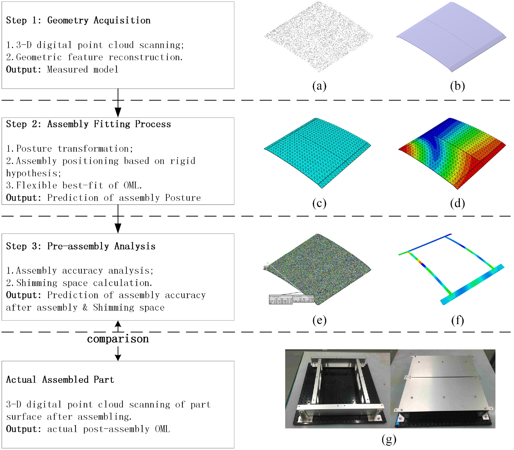
Overview of the proposed three-step method applied on thin-walled pieces: (a) scanning point cloud, (b) measured model, (c) actual shape mesh before assembly, (d) FEM for shape prediction after assembly, (e) assembly accuracy analysis, (f) Result of shimming, and (g) actual parts.

Definition and problem description

Definition of OML deviation and the clearance between the IML and the understructure

To meet the design requirements, the manufacturing process of the OML needs to be precisely controlled. A shim gap is required between the assembled understructure and the matched IML of the skin. The assembled framework and skin are shown in Figure 2. The shim space can be changed according to the assembly deviation of the understructure and the manufacturing deviation of the skin.

Figure 2.

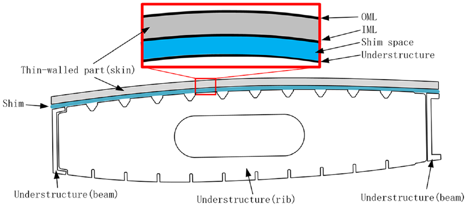
Assembled framework, skin, and shim structure.

The OML deviation refers to the normal deviation between the OML of actual thin-walled parts and the theoretical OML. The clearance between the IML and the understructure refers to the normal clearance between the IML of thin-walled parts and the understructure. Specifically, two surfaces, $S_{\mathrm{IML}}$ and $S_{\mathrm{uds}}$ , are involved. For points $C_j$ on the surface $S_{\mathrm{IML}}$ , the nearest point $P_j$ can be found on the surface $S_{\mathrm{uds}}$ (Figure 3). The length $\left|P_j{C}_j\right|$ is the distance from the surface $S_{\mathrm{IML}}$ to the surface $S_{\mathrm{uds}}$ at point $C_j$ . The nearest point $P_j$ on the surface $S_{\mathrm{uds}}$ can be expressed as follows:

$$\arg \min \Vert C_j-P_j\Vert ,P_j\in S_{\mathrm{uds}}$$

(1)

Figure 3.

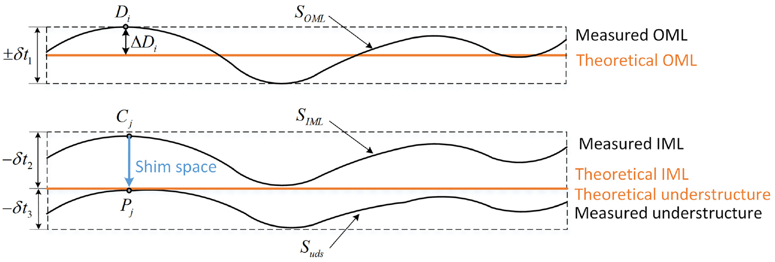
Definitions of measured OML, IML, and understructure.

The assembly clearance value of point $C_j$ is defined as:

$$G_j=\Vert P_j-C_j\Vert$$

(2)

Problem description

The sensitivity matrix of parts can be generated using different methods (i.e. empirical and mathematical methods). In this study, a Finite Element Model (FEM) based on the measured model was constructed, which was used in the simulation of the assembly stage. The degree of freedom is defined as the points in the actual measured model of the part, the positioning connection between the fixture and the part, the part requirements, and the degree of freedom of each point. These points are transformed into the corresponding nodes of the FEM so that only the sensitivity matrix of the points of interest is obtained as follows:

$$\left[K\right]\left[\begin{array}{c}\Delta C_j\hfill \\ \multicolumn{1}{c}{\Delta D_i}\end{array}\right]=\left[\begin{array}{c}0\hfill \\ \multicolumn{1}{c}{F}\end{array}\right]$$

(3)

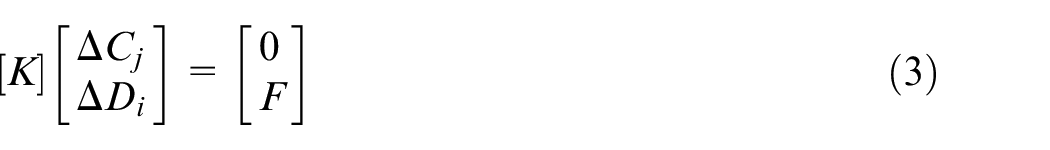
where K is the overall stiffness matrix, ΔC_j is the change in point C_j on IML, ΔD_i is the change in point D_i on the OML, and F is the virtual force at point D_i.

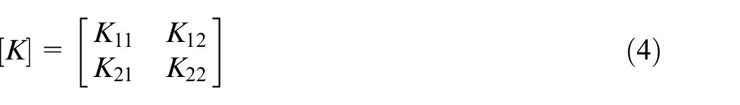
The overall stiffness matrix K is decomposed as follows:

$$\left[K\right]=\left[\begin{array}{cc}{K}_{11}\hfill & K_{12}\hfill \\ \multicolumn{1}{c}{K_{21}}& K_{22}\hfill \end{array}\right]$$

(4)

Substituting (4) into (3), we obtain:

$$\left[\Delta C_j\right]=-{\left[K_{11}\right]}^{-1}\left[K_{12}\right]\left[\Delta D_i\right].$$

(5)

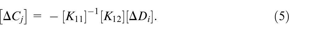
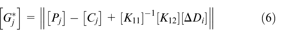
When (5) is substituted into (2), the clearance between the IML and the understructure is obtained under the condition of OML deformation, ΔD_i, as follows:

$$\left[G_j^{*}\right]=\Vert \left[P_j\right]-\left[C_j\right]+{\left[K_{11}\right]}^{-1}\left[K_{12}\right]\left[\Delta D_i\right]\Vert$$

(6)

Acquisition of geometric information from part surface

3D Digital point cloud scanning

3D scanning technology can be used to obtain 3D geometric information of the surface of objects. In recent decades, with the development and wide application of large-scale measurement technology in aerospace and other manufacturing industries,^4,5 the use of laser scanners or photogrammetric instruments has made it easy to obtain dense part point clouds,^6–8 providing important technical support for the acquisition of the geometry information of part surfaces.

The point cloud data collected by a laser digitizer is subjected to post-processing steps, such as denoising, simplification, and segmentation. ⁹ Owing to the inevitable existence of some noises in the scanning process, the shape of the object determined from these data often deviates from the actual shape; thus, some of the information could be redundant. To reduce the impact of these points on the subsequent data processing, it is necessary to remove them. In general, to achieve a better feature extraction effect, the point cloud data also need to be filtered. Typical filtering methods used for denoising include the median filter, mean filter, standard Gaussian filter, and adaptive filter. ¹⁰

With the development of 3D scanning technology, the measurement accuracy and scanning efficiency of the equipment have been gradually improved by point cloud data simplification. The collected 3D points on the surface of the object are dense, and most of them are redundant. If the characteristics of the object are not affected, simplification of the point cloud data can improve the data processing efficiency. Commonly used simplification methods are classified into three categories: direct simplification method, ¹¹ surface fitting-based simplification algorithm,^12–14 and mesh-based simplification algorithm.^15,16

Owing to the large amount of collected point cloud data, the feature information is not clear, and the subsequent processing is difficult. Therefore, it is necessary to segment the point cloud for subsequent processing. Currently used point cloud segmentation algorithms are mainly divided into model decomposition algorithms based on boundary features,^17,18 segmentation algorithms based on region growth,^19,20 clustering algorithms based on feature solution,^21,22 and segmentation algorithms based on rigid features of topology.^23,24

In this study, the digital measurement process was performed using a Leica T-Scan 5, with the following features: spatial length measurement uncertainty (2 sigma): UL = 60 μm (<8.5 m), UL = 26 μm + 4 μm/m (>8.5 m); uncertainty of sphere radius measurement (2 sigma): UR = 50 μm (<8.5 m), UR = 16 μm +4 μm/m (>8.5 m), US = 85 μm + 1.5 μm/m; plane measurement uncertainty (2 sigma): UP = 80μm+ 3μm/m.

The measurement system consists of a laser tracker, T-scan, scanning measurement software, and measurement auxiliary tools. The laser tracker and its control system were used to establish the measurement field. A T-scan laser scanner and its control system were used to scan the IML, OML, and understructure, as shown in Figure 4.

Figure 4.

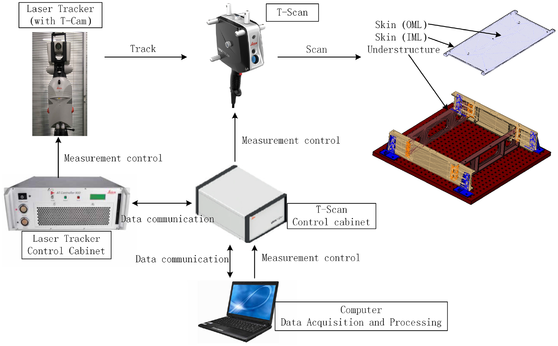
Laser scanning system.

Reconstruction of geometric features of parts

Point cloud data can be used to analyze the manufacturing deviation of parts as well as to reverse build the measured model. In this paper, the point cloud data of the parts was used to reconstruct their geometric features and build the measured model for the subsequent assembly analysis and OML control.

In recent years, many scholars have proposed many surface reconstruction algorithms. Surface reconstruction methods are usually divided into implicit surface reconstruction methods^25,26 and triangular mesh reconstruction methods. ²⁷ In this study, the non-uniform rational B-spline (NURBS) surface fitting method was used for reconstruction. NURBS is an excellent modeling method which is supported by advanced 3D software. NURBS can better control the curvilinear degree of an object surface than the mesh modeling method, thus generating a more realistic and vivid shape.

The reconstructed model was also used for simulation analysis. Borhen et al. ²⁸ and Aicha et al. ²⁹ reconstructed the CAD model of a product based on B-spline by combining the results of the finite element analysis and the actual deviation of the parts. The simulation was performed based on the actual product.

Based on point cloud segmentation, the surface of each subpoint cloud was reconstructed and the complete surface model was then constructed by Boolean operation combined with each reconstruction patch. Finally, the solid was filled to obtain the complete measured model, as shown in Figure 5.

Figure 5.

Construction process of measured model: (a) point cloud segmentation, (b) surface reconstruction, and (c) solid fill (measured model).

Analysis of reconstruction accuracy

Various errors are involved in the entire model reconstruction process. From the acquisition of measurement data to the final reconstructed model, the following errors are mainly observed: prototype manufacturing error ${\Delta }_{\mathrm{ma}}$ , measurement error ${\Delta }_{\mathrm{me}}$ , data processing error ${\Delta }_{\mathrm{dp}}$ , modeling error ${\Delta }_{\mathrm{mo}}$ , and compensation error ${\Delta }_{\mathrm{co}}$ .

A standard part can be reconstructed with a known manufacturing accuracy, ${\Delta }_{\mathrm{ma}}$ . The measurement error was mainly due to the low accuracy of the measurement equipment. Therefore, suitable digital measurement equipment should be selected according to the reconstruction requirements based on the total error. The data processing error ${\Delta }_{\mathrm{dp}}$ mainly refers to the error caused by smoothing, denoising, simplification, relocation, and other operations on the measured data. A compensation error ${\Delta }_{\mathrm{co}}$ exists only in the contact measuring equipment. During the measurement of a spatial free-form surface, the compensation error results from the probe radius compensation.

The surface modeling error is denoted as ${\Delta }_{\mathrm{mo}}$ . Planes, cylinders, etc., can be expressed by an accurate mathematical formula without any modeling error. A free-form surface cannot be simply expressed using a mathematical formula. Generally, the spline function or an NURBS patch is used for fitting which produces an error. The more complex the free-form surface, the greater the fitting error. The splicing between different surface patches also produces errors. These surface deformation errors in surface reconstruction are collectively referred to as the modeling error. In the process of free-form surface modeling, the modeling error is the main parameter that can control the surface fitting deviation. It is also a significant factor that affects the total error in the entire reconstruction process. Precision control mainly focuses on the modeling error.

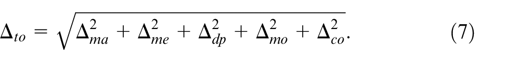
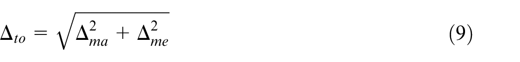
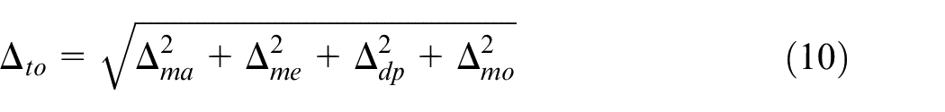
The total error between the reconstructed model and the physical sample is the cumulative error of each link. In general, all types of errors follow a normal distribution. The root mean square of each error can be defined as the precision error, that is, the precision quantitative index, as follows:

$${\Delta }_{\mathrm{to}}=\sqrt{{\Delta }_{\mathrm{ma}}^2+{\Delta }_{\mathrm{me}}^2+{\Delta }_{\mathrm{dp}}^2+{\Delta }_{\mathrm{mo}}^2+{\Delta }_{\mathrm{co}}^2}.$$

(7)

The weight of each error in this equation cannot be easily determined in the actual reconstruction; therefore, it is treated according to the equal weight. However, because the accurate size of each error cannot be determined easily, the accurate reconstruction accuracy cannot be estimated using this accuracy quantification index. Therefore, in practical engineering, the distance from the measuring point to the reconstructed surface is often used as the accuracy evaluation index of the reconstructed model, and its specific indices can be expressed by the average distance, maximum distance, standard deviation, etc.

During model reconstruction, the measurement data of the whole model was divided into point cloud data of the regular surface (plane, cylinder) and the free-form surface. Three reconstruction experiments are designed for the plane, cylindrical, and free-form surfaces to verify the accuracy of the model reconstruction.

Verification of reconstruction accuracy of plane parts

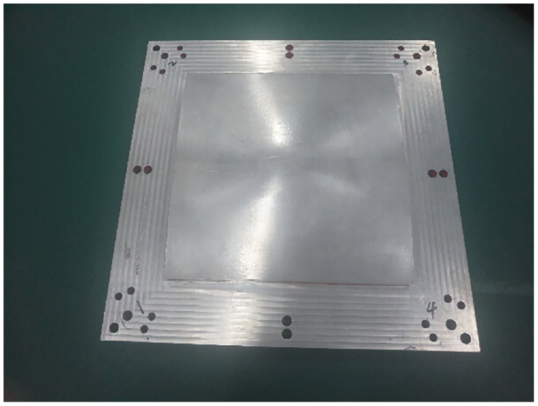
The flatness of the plane test piece was ±0.01 mm, as shown in Figure 6. Leica T-scan 5 was used for the measurement.

Figure 6.

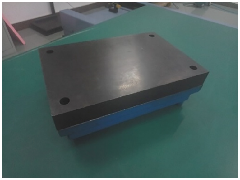
Plane parts.

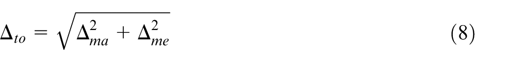
In the proposed accuracy evaluation model, the source of the reconstruction error of plane parts was analyzed. The prototype manufacturing error ${\Delta }_{\mathrm{ma}}$ of plane parts was 0.01 mm. When T-scan was used for digital measurement, a measurement accuracy of 0.0478 mm was achieved by T-scan within a distance of 3 m from the laser tracker. Furthermore, ${\Delta }_{\mathrm{me}}$ was 0.0478 mm. The point cloud in the experiment was not subjected to splicing or data processing. The T-scan did not require radius compensation and the plane fitting has no shape reconstruction error. Therefore, ${\Delta }_{\mathrm{dp}}$ , ${\Delta }_{\mathrm{mo}}$ , and ${\Delta }_{\mathrm{co}}$ are zero. Accordingly, the total error of plane reconstruction in this experiment is given as follows.

$${\Delta }_{\mathrm{to}}=\sqrt{{\Delta }_{\mathrm{ma}}^2+{\Delta }_{\mathrm{me}}^2}$$

(8)

According to the plane reconstruction theory, the total error that can be achieved using the T-scan measurement data is 0.049 mm. The experimental verification is performed as follows.

To achieve the best measurement accuracy considering the accuracy of the T-scan, it was important to ensure that the T-scan is within 3 m from the laser tracker and approximately 150 mm from the surface of the plane parts during scanning. After the measurements, the least square fitting point cloud was used to form a plane.

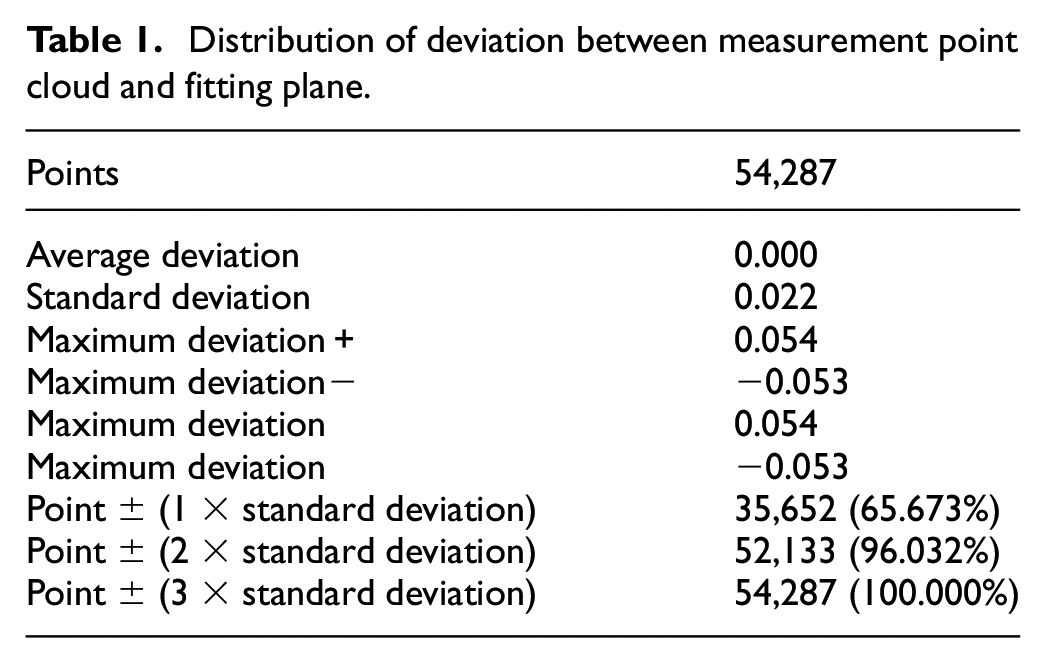
The measured data point cloud and the fitted plane were imported into PolyWorks for deviation detection. The deviation color map between the measured point cloud and the reconstructed model was obtained as shown in Figure 7 and Table 1. The point cloud deviation statistics were then determined. Table 1 shows that the maximum deviation from the point to the plane was 0.054 mm, minimum deviation was −0.053 mm, standard deviation was 0.022 mm, and the number of points whose deviations were distributed within twice the standard deviation (sigma) was 96.032%.

Table 1.

Distribution of deviation between measurement point cloud and fitting plane.

Points	54,287
Average deviation	0.000
Standard deviation	0.022
Maximum deviation+	0.054
Maximum deviation−	−0.053
Maximum deviation	0.054
Maximum deviation	−0.053
Point ± (1 × standard deviation)	35,652 (65.673%)
Point ± (2 × standard deviation)	52,133 (96.032%)
Point ± (3 × standard deviation)	54,287 (100.000%)

Figure 7.

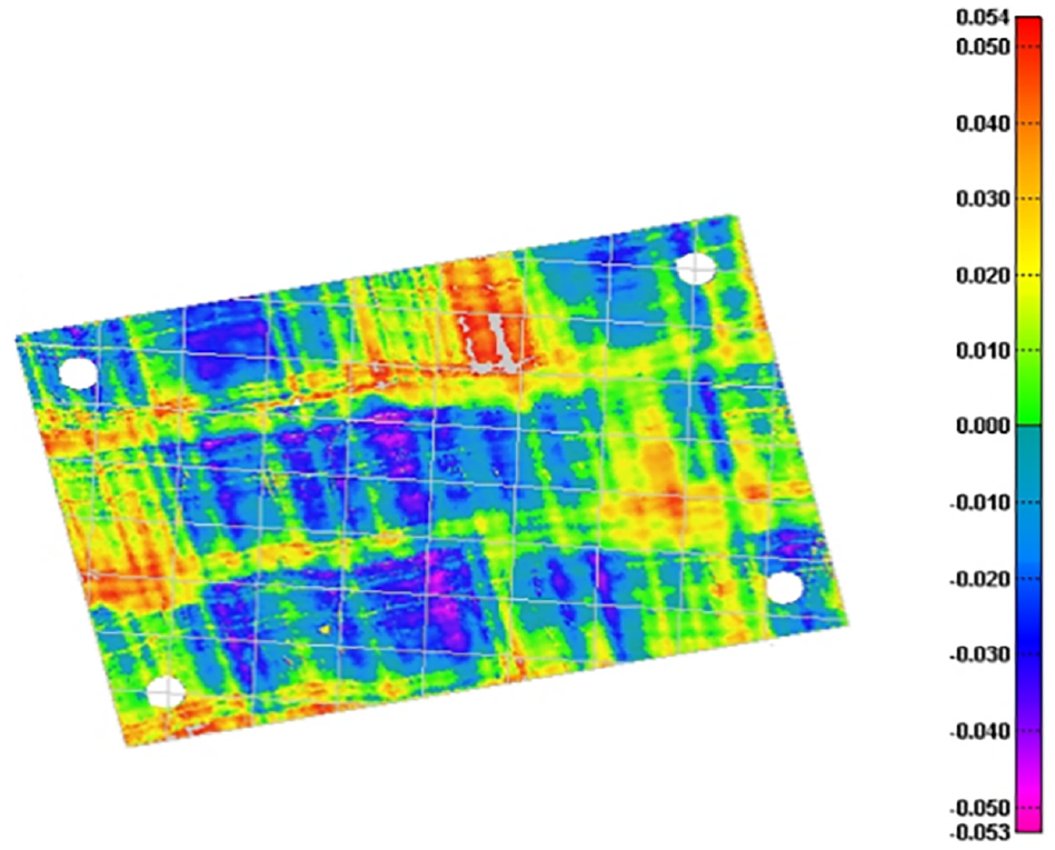
Color map of measurement point cloud and reconstruction plane deviation.

If the distance from the measuring point to the reconstructed plane is considered as the basis for evaluating accuracy and the maximum deviation is adopted as the index, the reconstruction accuracy of the plane part based on the T-scan measuring point cloud is ±0.054 mm.

Verification of reconstruction accuracy of cylindrical parts

The accuracy of the cylindrical test pieces as shown in Figure 8 is ±0.001 mm. The radii of the pieces, from left to right are 12, 15, and 16 mm, respectively. Leica T-scan 5 is used for the measurements.

Figure 8.

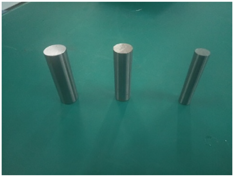
Cylindrical test pieces with accuracy of 0.001 mm.

According to the proposed accuracy evaluation model, the source of the reconstruction error in the plane parts was analyzed. The prototype manufacturing error, ${\Delta }_{\mathrm{ma}}$ , of the cylindrical surface was 0.001 mm. When employing T-scan for the digital measurement equipment, a measurement accuracy of 0.0478 mm can be achieved by using the T-scan within 3 m from the laser tracker; thus, ${\Delta }_{\mathrm{me}}$ is 0.0478 mm. The point cloud in the experiment does not involve splicing or data processing. The T-scan does not require radius compensation and the plane fitting has no shape reconstruction errors. Thus, ${\Delta }_{\mathrm{dp}}$ , ${\Delta }_{\mathrm{mo}}$ , and ${\Delta }_{\mathrm{co}}$ are zero. Therefore, the total error quantification model for the cylindrical reconstruction in this experiment is

$${\Delta }_{\mathrm{to}}=\sqrt{{\Delta }_{\mathrm{ma}}^2+{\Delta }_{\mathrm{me}}^2}$$

(9)

The total error in the plane reconstruction theory determined using the T-scan measurement data was 0.049 mm. The experimental verification is presented below.

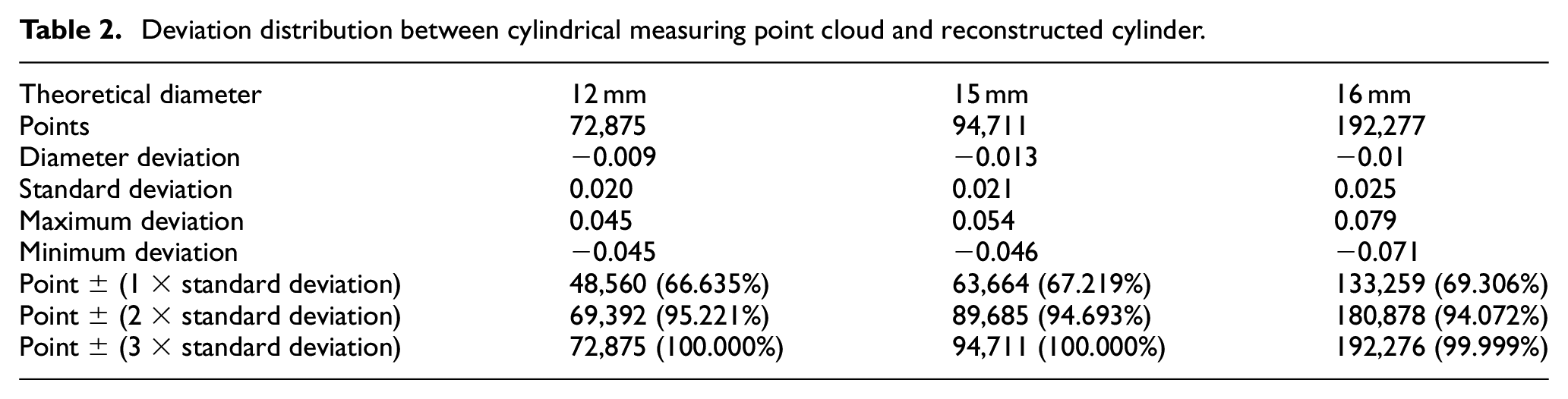
The point cloud data and the reconstructed model were then imported into PolyWorks for deviation detection and the color map of the deviation between the measured point cloud and the reconstructed model was obtained as shown in Figure 9. The statistical information pertaining to the deviation between the point cloud and the reconstructed cylinder is presented in Table 2. As shown in Table 2, the diameter deviation for the cylindrical surface with a diameter of 12 mm was −0.009 mm, standard deviation was 0.02 mm, and the number of points with deviations within twice the standard deviation was 95.221%. Furthermore, the diameter deviation for the cylindrical surface with a diameter of 15 mm was −0.013 mm, standard deviation was 0.021 mm, and the number of points with deviations within twice the standard deviation was 94.693%. Lastly, the diameter deviation for the cylindrical surface with a diameter of 16 mm was −0.01 mm, standard deviation was 0.025 mm, and the number of points with deviations within twice the standard deviation was 94.072%.

Table 2.

Deviation distribution between cylindrical measuring point cloud and reconstructed cylinder.

Theoretical diameter	12 mm	15 mm	16 mm
Points	72,875	94,711	192,277
Diameter deviation	−0.009	−0.013	−0.01
Standard deviation	0.020	0.021	0.025
Maximum deviation	0.045	0.054	0.079
Minimum deviation	−0.045	−0.046	−0.071
Point ± (1 × standard deviation)	48,560 (66.635%)	63,664 (67.219%)	133,259 (69.306%)
Point ± (2 × standard deviation)	69,392 (95.221%)	89,685 (94.693%)	180,878 (94.072%)
Point ± (3 × standard deviation)	72,875 (100.000%)	94,711 (100.000%)	192,276 (99.999%)

Figure 9.

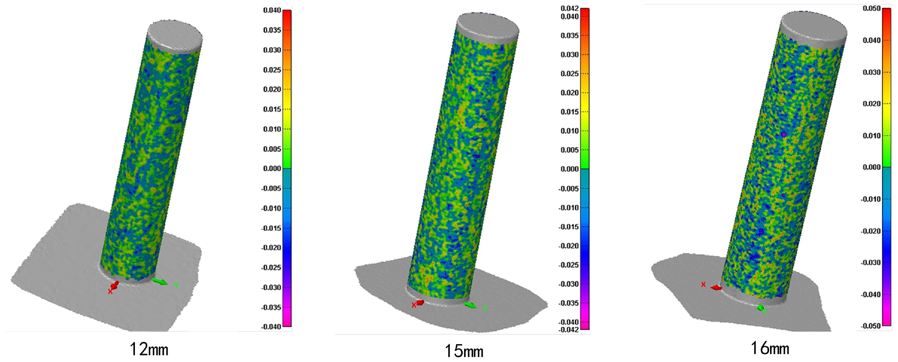
Cylindrical measurement point cloud and reconstructed cylindrical deviation color maps.

The maximum diameter deviation for the reconstructed cylinder was 0.013 mm, maximum standard deviation was 0.025 mm, and the number of points with ±2 × standard deviation was greater than 94%. Considering twice the standard deviation distance as the basis for the accuracy evaluation, the geometric reconstruction accuracy of the cylindrical parts was found to be ±0.05 mm.

Verification of reconstruction accuracy of free-form surface

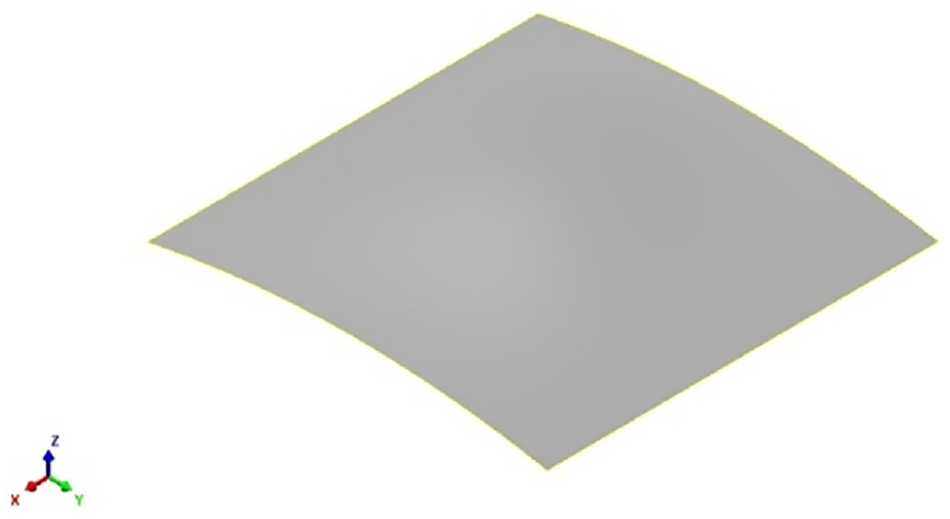
The surface profile of the free-form surface test piece was ±0.05 mm, as shown in Figure 10. Leica T-scan 5 was used for the measurements.

Figure 10.

Free-form surface parts.

Using the proposed accuracy evaluation model, the error sources of the free-form surface reconstruction were analyzed. The reconstruction errors of the free-form surface included the manufacturing error, ${\Delta }_{\mathrm{ma}}$ , which is 0.05 mm in this experiment. When employing T-scan for the digital measurement equipment, a measurement accuracy of 0.0478 mm was achieved by using the T-scan within 3 m from the laser tracker. Thus, ${\Delta }_{\mathrm{me}}$ is 0.0478 mm. The actual position and theoretical position of the free-form surface parts was determined using the datum point alignment method. For the measurement of the datum point, the 0.5-inch target ball of the laser tracker was employed creating an alignment error. Prior to fitting the surface with the free-form surface point cloud, it was necessary to first smooth and denoise the point cloud. If smoothing errors exist, the data processing error is ${\Delta }_{\mathrm{dp}}=\sqrt{{\Delta }_{\mathrm{alignment}}^2+{\Delta }_{\mathrm{smooth}}^2}$ . Finally, the surface was fitted, resulting in the modeling error, ${\Delta }_{\mathrm{mo}}$ . Therefore, the error model of the free-form surface reconstruction based on T-scan equipment is:

$${\Delta }_{\mathrm{to}}=\sqrt{{\Delta }_{\mathrm{ma}}^2+{\Delta }_{\mathrm{me}}^2+{\Delta }_{\mathrm{dp}}^2+{\Delta }_{\mathrm{mo}}^2}$$

(10)

The T-scan equipment was adopted to scan the surface part in order to obtain the surface measurement point cloud data. Four datum points were used to align the measurement point cloud with the digital analog. The alignment error associated with the datum point was 0.019 mm. Subsequently, the point cloud was triangulated, the vertices are smoothed, and noise was eliminated. Furthermore, an allowable displacement error of 0.05 mm was selected and the surface was finally fit. The reconstructed surface was obtained via NURBS patch fitting, as shown in Figure 11.

Figure 11.

NURBS surface reconstruction.

The quality of the reconstructed surface was also evaluated. Based on Figures 12 and 13, the zebra stripes and the curvature distribution map of the reconstructed surface indicated that a good curvature fairing effect of the reconstructed surface and good continuity; hence, the reconstructed surface exhibits better surface reconstruction quality.

Figure 12.

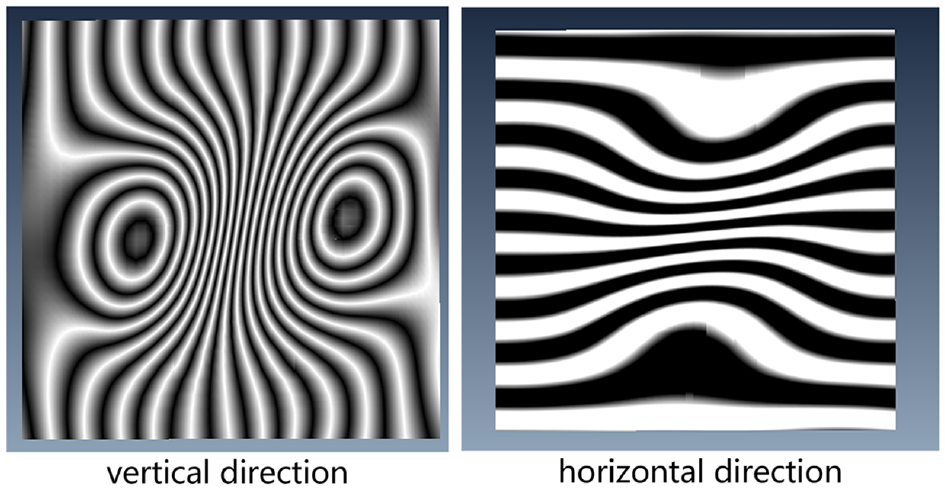
Zebra stripes for reconstructed surface.

Figure 13.

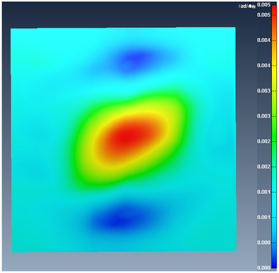
Curvature distribution for reconstructed surface.

Subsequently, the accuracy of the reconstructed surface was verified. First, the reconstructed surface was discretized into a point cloud. It was then imported into PolyWorks for deviation detection and the reference object was the theoretical model of the curved surface parts. As shown in Figure 14, the deviation color map, surface profile, and maximum and minimum deviation values was obtained.

Figure 14.

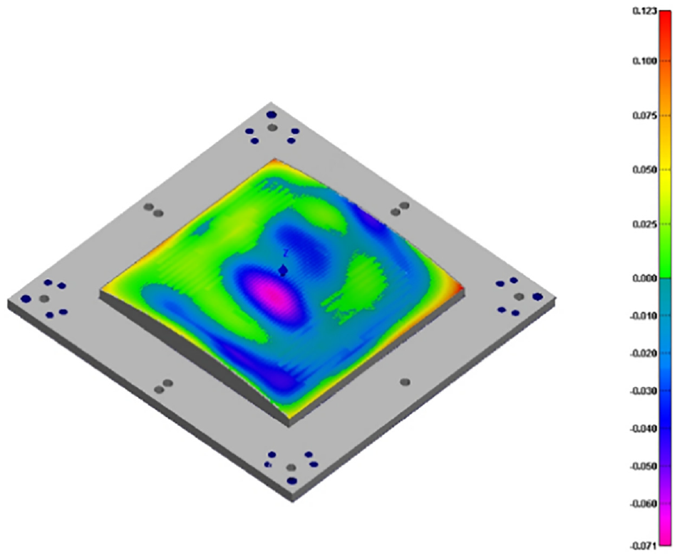
Color map of deviation between discrete points of the reconstructed surface and theoretical surface.

According to the comparison results of the deviation between the discrete point clouds of the reconstructed surface and the theoretical surface, the maximum deviation of the reconstructed surface was 0.075 mm and minimum deviation was −0.072 mm. The accuracy of the reconstructed surface is expressed by the surface profile of the discrete point cloud in the deviation detection. Hence, the overall reconstruction accuracy of the reconstructed surface is ±0.075 mm.

Assembly fitting process for thin-walled parts

The principle for the location fitting of thin-walled parts involves the transformation of the local coordinate system into the global coordinate system. However, owing to their low rigidity, thin-walled parts often undergo deformation in the assembly process. This is typically caused by manufacturing deviations, the spring back effect, gravity, and the stresses generated during assembly. The general method for location fitting during rigid structure assembly affords the best fitting under the premise that the relative position of the local coordinate system and the key points remains unchanged. Because there are certain uncertainties associated with the assembly process of thin-walled parts, it is necessary to develop new methods to account for the influence of these uncertainties to ensure the accuracy and effectiveness of location fitting. The assembly fitting algorithm proposed herein is a process of successive approximation which includes two steps: the fitting process based on the rigid assumption and the fitting process based on the flexible best fitting. A flowchart of this algorithm is depicted in Figure 15. After the fitting, the rigid transformation matrix and the flexible node coordinates of the finite element model are obtained as the output.

Figure 15.

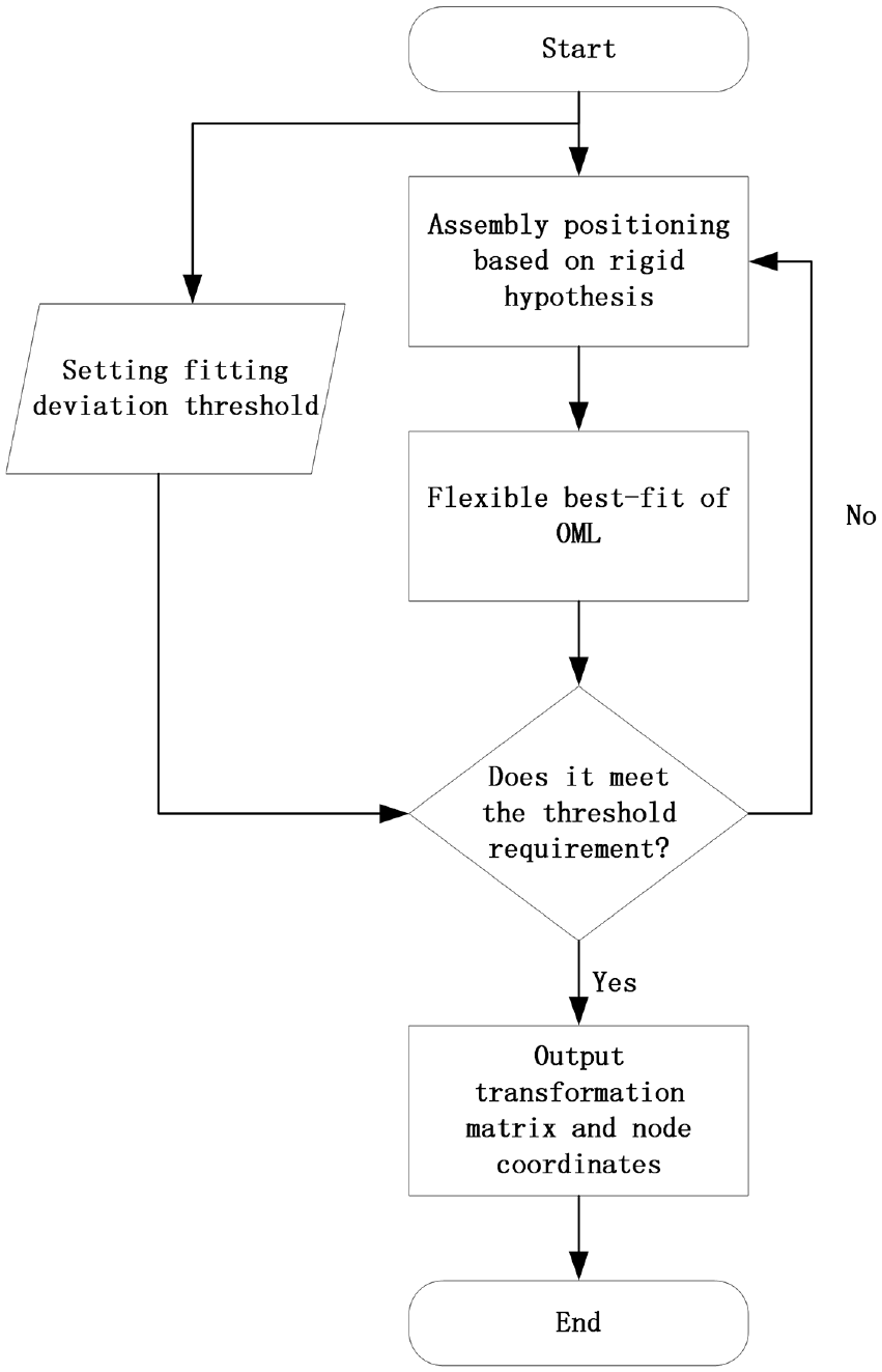
Assembly fitting process for thin-walled parts.

Posture transformation

The posture of an aircraft skin assembly describes the relative spatial position and pose the relationship between the skin and the framework. The spatial posture of a rigid body can be represented by its fixed coordinate system. Therefore, the posture of a skin assembly can be expressed as the posture transformation relationship between the fixed coordinate system { A } on the skin and the fixed coordinate system { B } on the framework.

The coordinates of space points in different coordinate systems vary. The measured data of the skin lie in the coordinate system of the skin itself. To coordinate the calculation of the assembly, all the data points need to be converted into a unified assembly coordinate system. Considering the transformation of any point p on skin { A } to the framework coordinate system { B } as an example, the transformation relationship can be expressed as follows:

$${}^B\mathbf{P}={}_A{}^B\mathit{R}·\mathit{p}+{{}^B\mathit{t}}_{\mathrm{Ao}}$$

(11)

The abovementioned formula denotes the translation and rotation composite transformation of p from { A } to { B }. ${}_A{}^B\mathit{R}=I$ represents the translation transformation, and ${{}^B\mathit{t}}_{\mathrm{Ao}}=0$ represents the rotation transformation. The composite transformation in (11) is nonhomogeneous to point p , which, in the homogeneous form, can be expressed as:

$$\left[\begin{array}{c}{}^B\mathbf{P}\hfill \\ \multicolumn{1}{c}{---}\\ \multicolumn{1}{c}{1}\end{array}\right]=\left[\begin{array}{cc}{}_A{}^B\mathit{R}\hfill & {{}^B\mathit{t}}_{\mathrm{Ao}}\hfill \\ \multicolumn{1}{c}{\begin{array}{ccc}0\hfill & 0\hfill & 0\hfill \end{array}}& 1\hfill \end{array}\right]\left[\begin{array}{c}\mathit{p}\hfill \\ \multicolumn{1}{c}{---}\\ \multicolumn{1}{c}{1}\end{array}\right]$$

(12)

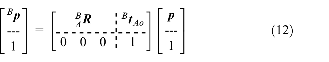
Among these, the 4 × 1 column vector is the homogeneous form of the three-dimensional space points, which is still recorded as $\mathit{p}$ or ${}^B\mathbf{P}$ . The 4 × 4 homogeneous transformation matrix ${}_A{}^B\mathit{T}$ can be written as:

$${}_A{}^B\mathit{T}=\left[\begin{array}{cc}{}_A{}^B\mathit{R}\hfill & {{}^B\mathit{t}}_{\mathrm{Ao}}\hfill \\ \multicolumn{1}{c}{\begin{array}{ccc}0\hfill & 0\hfill & 0\hfill \end{array}}& 1\hfill \end{array}\right]$$

(13)

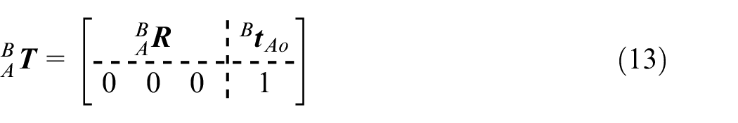
The translation and rotation from { A } to { B } are synthetically represented. ${}_A{}^B\mathit{T}$ is also the equivalent expression of the skin coordinate system { A } relative to the framework coordinate system { B } assembly pose $\mathit{t}={\left[\begin{array}{cc}\begin{array}{ccc}x\hfill & y\hfill & z\hfill \end{array}\hfill & \begin{array}{ccc}\alpha \hfill & \beta \hfill & \gamma \hfill \end{array}\hfill \end{array}\right]}^T$ .

Assembly positioning based on rigid hypothesis

In this study, under the premise of digital assembly, two holes and one surface were used to locate the parts. The surface represented the main positioning (A), hole I was the second positioning reference (B), and hole II was the third positioning reference (C), as shown in Figure 16. First, the main positioning surface (A) and positioning datum (A’) of the part were fitted using the ICP algorithm. ³⁰ The transformation matrix is:

$${\mathit{T}}_1=\left[\begin{array}{cc}{\mathit{R}}_1\hfill & {\mathit{t}}_1\hfill \\ \multicolumn{1}{c}{\begin{array}{ccc}0\hfill & 0\hfill & 0\hfill \end{array}}& 1\hfill \end{array}\right]$$

(14)

Figure 16.

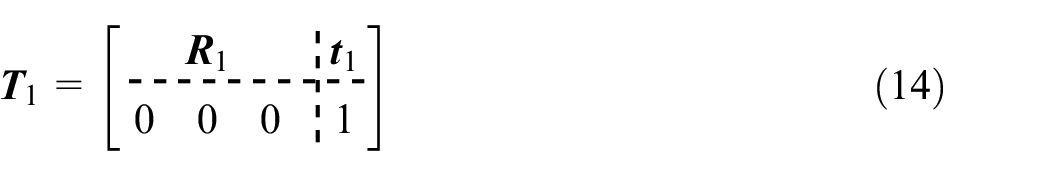
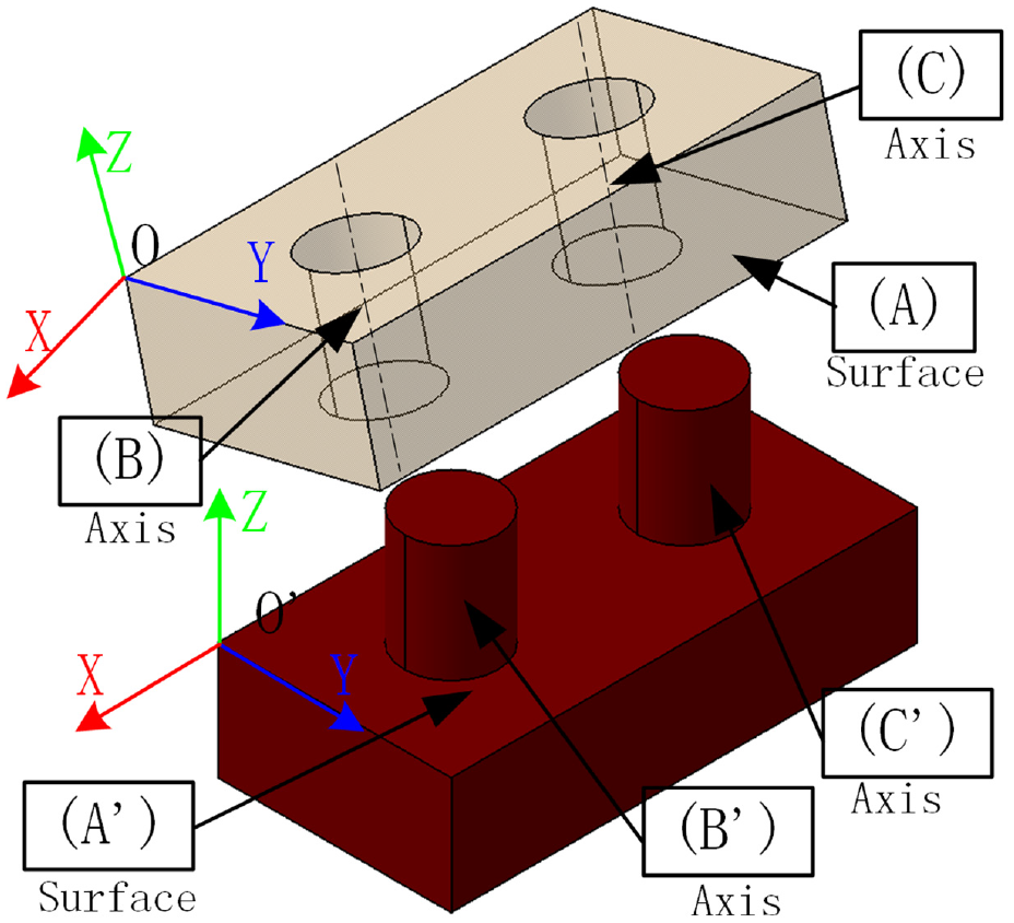
Assembly positioning based on rigid hypothesis.

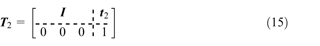
Then, the part is translated using a vector from the hole (B) to the positioning datum (B′). The transformation matrix is:

$${\mathit{T}}_2=\left[\begin{array}{cc}\mathit{I}\hfill & {\mathit{t}}_2\hfill \\ \multicolumn{1}{c}{\begin{array}{ccc}0\hfill & 0\hfill & 0\hfill \end{array}}& 1\hfill \end{array}\right]$$

(15)

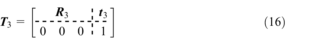
Finally, the rotation angle is calculated according to the hole (C) and positioning datum (C′). The transformation matrix is:

$${\mathit{T}}_3=\left[\begin{array}{cc}{\mathit{R}}_3\hfill & {\mathit{t}}_3\hfill \\ \multicolumn{1}{c}{\begin{array}{ccc}0\hfill & 0\hfill & 0\hfill \end{array}}& 1\hfill \end{array}\right]$$

(16)

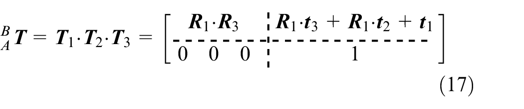
The transformation matrix of the parts from the initial to the final assembly is as follows:

$${}_A{}^B\mathit{T}={\mathit{T}}_1·{\mathit{T}}_2·{\mathit{T}}_3=\left[\begin{array}{cc}{\mathit{R}}_1·{\mathit{R}}_3\hfill & {\mathit{R}}_1·{\mathit{t}}_3+{\mathit{R}}_1·{\mathit{t}}_2+{\mathit{t}}_1\hfill \\ \multicolumn{1}{c}{\begin{array}{ccc}0\hfill & 0\hfill & 0\hfill \end{array}}& 1\hfill \end{array}\right]$$

(17)

Flexible best fit of OML

After the initial positioning based on the rigid body hypothesis, the flexible best fit of the OML was realized. An FEM based on triangular mesh elements was established using the octree algorithm, which reflects the actual shape and material characteristics of the parts. Subsequently, a set of OML constraints was defined as the boundary conditions to simulate the shape of the OML after assembly.

For example, for the positioning hole (B), (C) must be constrained during the skin assembly. For each location of i nodes D_i on the OML face of the mesh, these nodes should be forced to be placed on the theoretical OML after assembly.

During the finite element analysis, by applying a set of displacement boundary conditions, defined by the derived laws for rotation and translation, all the nodes in each group of D_i were forced on the theoretical OML. The resulting deformable mesh represents the predicted assembled shape of the component and can be used to derive the node C_j coordinates. The C_j coordinates of the nodes reflect the shape of the IML, for the case of an ideal OML, as shown in Figure 17.

Figure 17.

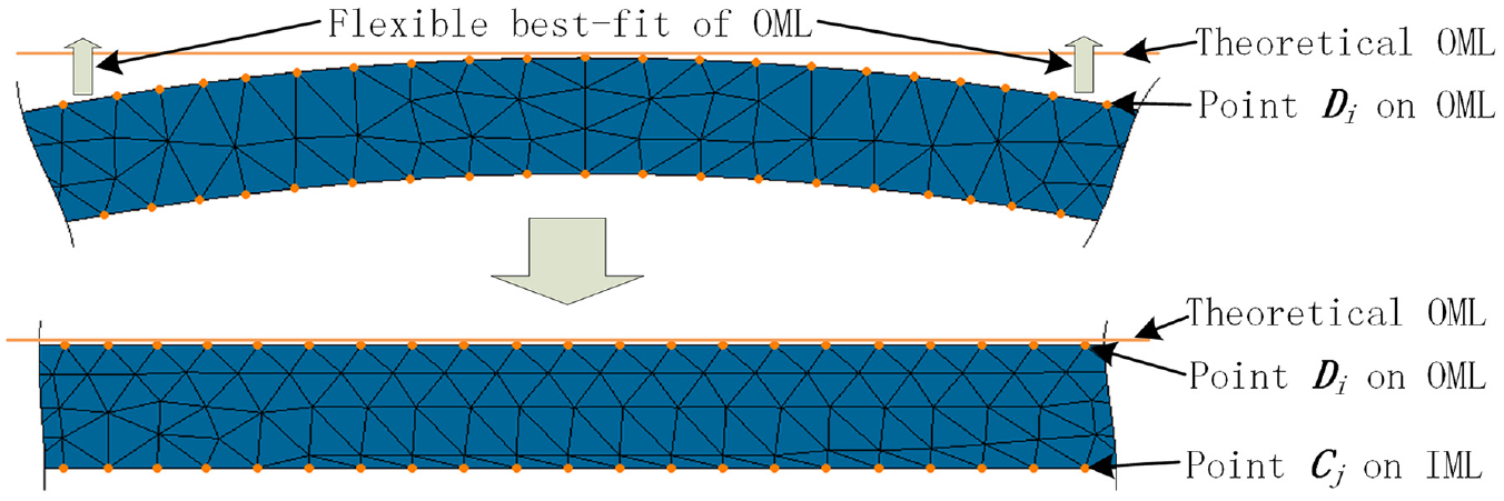
Flexible best-fit process for OML.

Physical verification

This section presents the verification of the proposed method. The structure and the size of the verification setup are shown in Figure 18. The verification setup consists of beam × 2, rib × 2, skin × 2, positioner × 4, adapter plate × 4, and flexible clamping platform × 1. The verification setup is shown in Figure 19.

Figure 18.

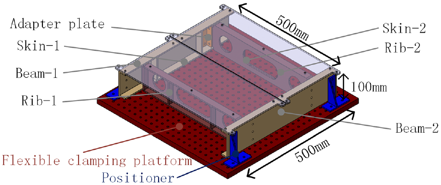
Structure of verification setup.

Figure 19.

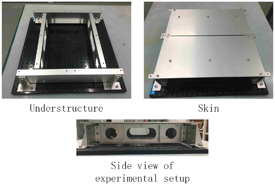
Verification setup.

The verification process is as follows. First, the framework (composed of the beam, rib, and adapter plate) was installed, and the understructure was measured. Second, the OML and IML of the skin were measured and the measured models were constructed. The posture and deformation of the skin after assembly are calculated using the method described in Sections 6.2 and 6.3. The process of shimming is simulated in accordance with artificial shimming. Finally, the skin assembly was completed and the OML after assembly was measured to verify the feasibility of the method.

Acquisition and processing of point clouds of parts

The method and equipment described in Section 4.1 was used to scan the skin and framework and obtain the actual pre-assembled shape. The reconstruction algorithm was used to reconstruct the surface. Figure 20 shows the deviations between the actual and theoretical shapes. The maximum deviation of Skin-1 was 3.017 mm and the average deviation was −0.115 mm. The maximum deviation of Skin-2 is 3.026 mm and the average deviation was −0.048 mm. The maximum deviation of Framework is 0.257 mm and the average deviation was 0.015 mm.

Figure 20.

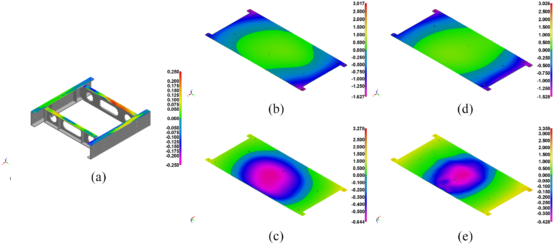
Deviations between actual and theoretical shapes: (a) framework under structure deviation, (b) Skin-1 OML deviation, (c) Skin-1 IML deviation, (d) Skin-2 OML deviation, and (e) Skin-2 IML deviation.

Using the method discussed in Section 4.3, the point cloud data of the skin and framework was reconstructed into the actual measured model, as shown in Figure 21.

Figure 21.

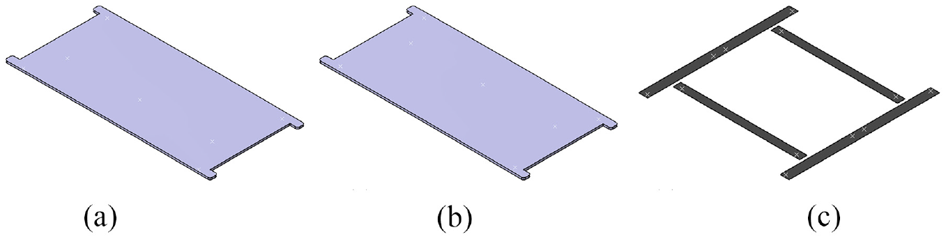
Measured models for (a) Skin-1, (b) Skin-2, and (c) Framework.

Skin and understructure assembly coordination

Global coordinate conversion

According to the coordinate transformation method proposed in Section 6.2, Skin-1 and Skin-2 are located in the global coordinate system. Hence, the skin and the framework are in the same coordinate system, as shown in Figure 22. Specifically, the IML of the skin is selected as the locating surface, and two holes are selected as the locating holes. Thereafter, the best fit was determined based on the rigid body assumption. The transformation matrices for Skin-1 and Skin-2 are as follows:

$$\begin{array}{c}\multicolumn{1}{c}{{}^{\mathrm{Framework}\mathrm{Skin}-1}\mathit{T}=\left[\begin{array}{cccc}0.984\hfill & -0.062\hfill & -0.169\hfill & -641.121\hfill \\ \multicolumn{1}{c}{0.163}& 0.700\hfill & 0.695\hfill & 235.476\hfill \\ \multicolumn{1}{c}{0.076}& -0.711\hfill & 0.699\hfill & -389.887\hfill \\ \multicolumn{1}{c}{0}& 0\hfill & 0\hfill & 1\hfill \end{array}\right],}\\ \multicolumn{1}{c}{{}^{\mathrm{Framework}\mathrm{Skin}-2}\mathit{T}=\left[\begin{array}{cccc}0.912\hfill & 0.369\hfill & -0.179\hfill & 1325.408\hfill \\ \multicolumn{1}{c}{0.328}& -0.918\hfill & -0.224\hfill & -195.813\hfill \\ \multicolumn{1}{c}{-0.247}& 0.145\hfill & -0.958\hfill & 272.203\hfill \\ \multicolumn{1}{c}{0}& 0\hfill & 0\hfill & 1\hfill \end{array}\right]}\end{array}$$

Figure 22.

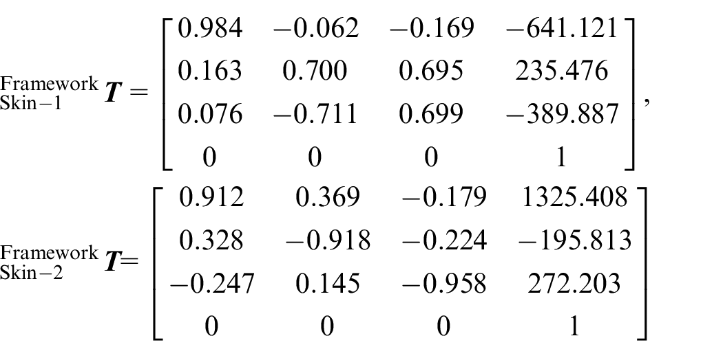
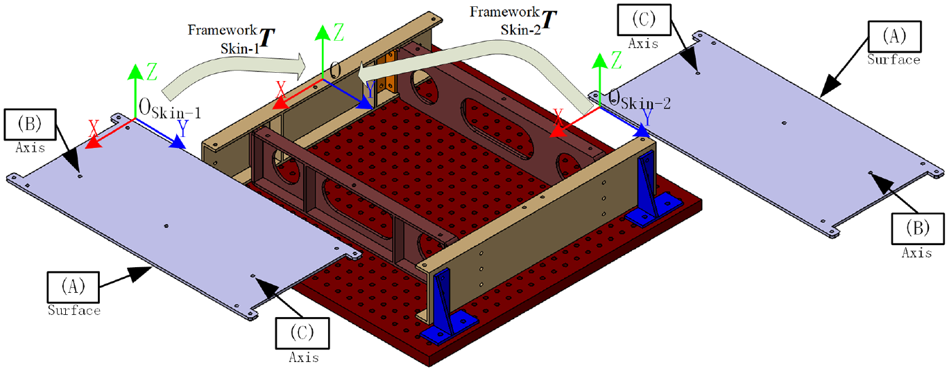
Skin-to-framework coordinate conversion.

Flexible best fit

The finite element analysis software ABAQUS was used for the flexible best fit. The four corner holes were constrained to realize the positioning of parts. Loads were added to the nodes of the OML in the measured model. The loads represented the deviation between the OML of the measured model and the theoretical one. Consequently, each node of the OML of the measured model coincided with the corresponding node of the theoretical OML. Subsequently, the node coordinates of the IML after flexible fitting were calculated using (3). The deformation of Skin-1 and Skin-2 after the flexible best fit is presented in Figure 23.

Figure 23.

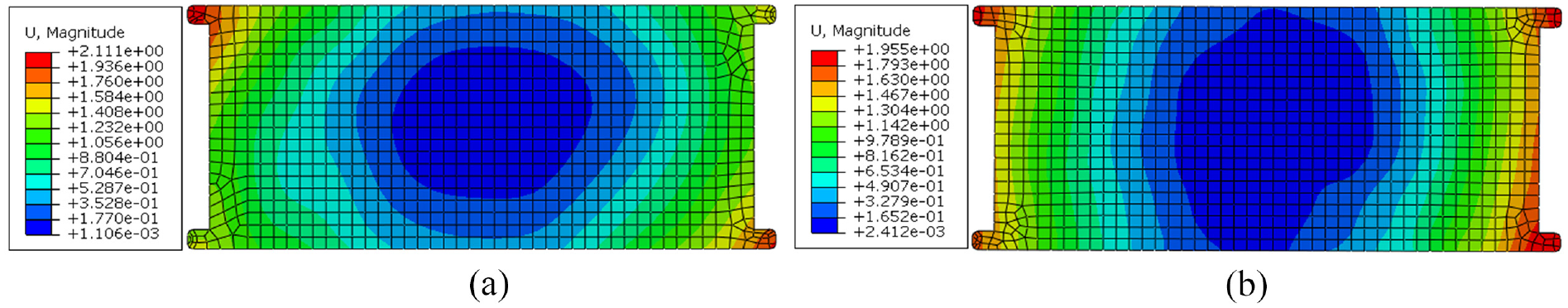
Deformation of Skin-1 and Skin-2 after flexible best fit: (a) Skin-1 deformation after flexible best-fit and (b) Skin-2 deformation after flexible best-fit.

OML control feasibility and results

The shimming value between the IML and the framework is calculated using (6), as shown in Figure 24. The results of positions ① to ⑧ are compared with the measurement results of the feeler gauge, as shown in Table 3. The process of artificial shimming is adopted. The OML deviation after shimming is depicted in Figure 25(b).

Table 3.

Comparison between calculated results and measured results.

Position number	Calculationresults (mm)	Measured results (mm)
①	0.23	0.25
②	0.14	0.15
③	0.22	0.20
④	0.08	0.10
⑤	0.14	0.15
⑥	0.08	0.05
⑦	0.06	0.05
⑧	0.27	0.25

Figure 24.

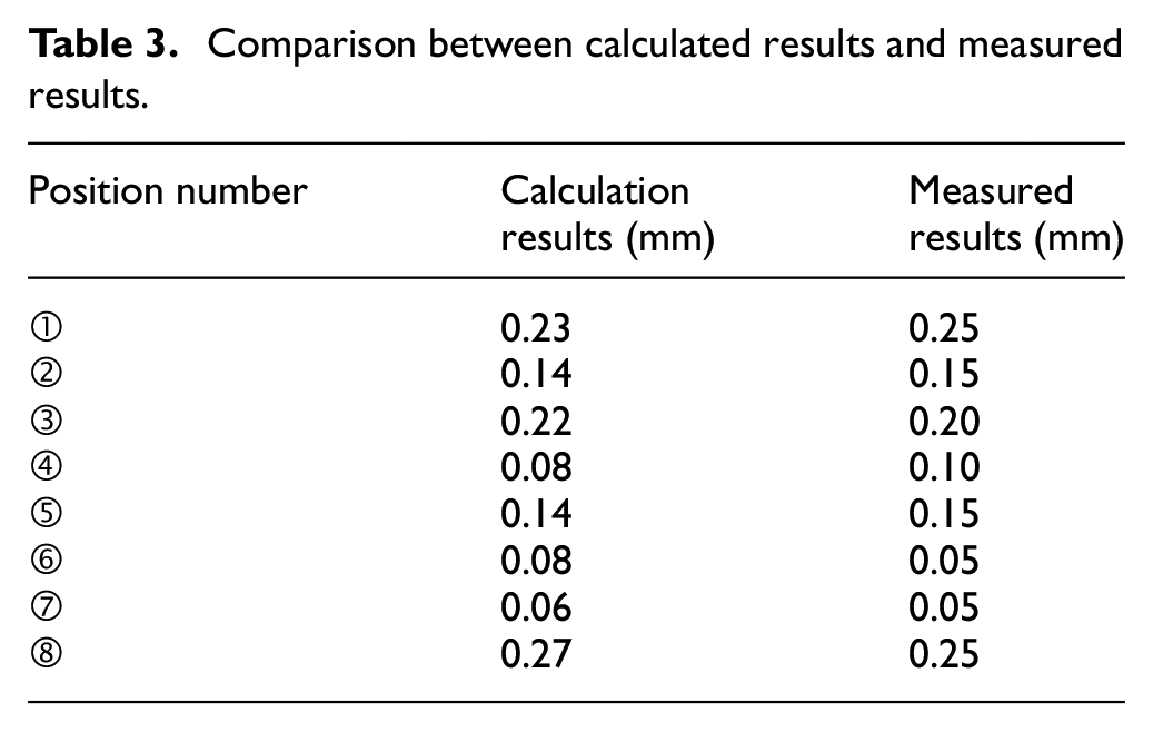
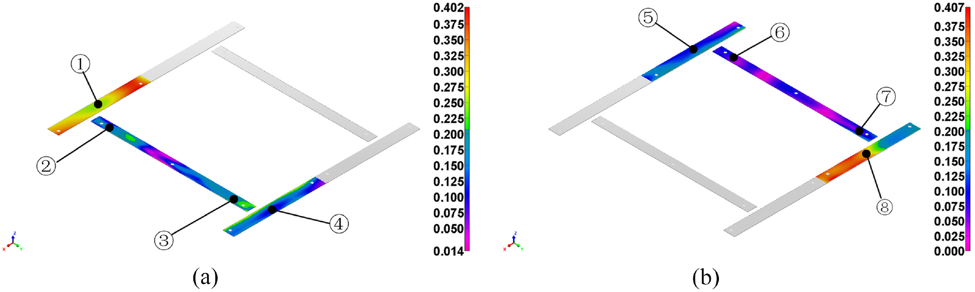
Shimming values of (a) Skin-1 and (b) Skin-2.

Figure 25.

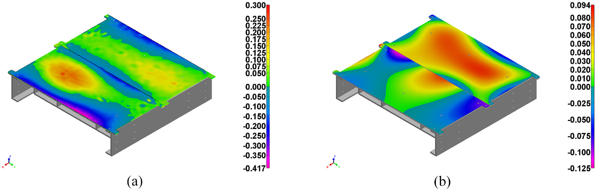
Comparison between assembly results without shimming and with shimming using the proposed method: (a) OML deviation after assembly without shimming and (b) OML deviation after assembly with shimming.

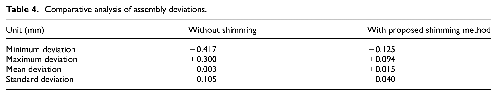
The assembly without shimming and the assembly after shimming using the proposed method are compared. The results reveal that the proposed method affords smaller deviations in the OML, as shown in Figure 25 and Table 4. The results also show that the proposed method can effectively control the OML of thin-walled parts.

Table 4.

Comparative analysis of assembly deviations.

Unit (mm)	Without shimming	With proposed shimming method
Minimum deviation	−0.417	−0.125
Maximum deviation	+0.300	+0.094
Mean deviation	−0.003	+0.015
Standard deviation	0.105	0.040

Conclusions

In this work, a method of shimming based on the OML control of thin-walled parts is developed. This approach can predict the shape of a shimming space via the virtual assembly of thin-walled parts in their final assembly state. 3D digital scanning equipment is used to measure the shape before assembly and the measured finite element model is generated to analyze the shape after assembly. The shimming space is then obtained and a verification step is performed by comparing the predicted and actual assembled shapes. Physical verification reveals that this method can predict the shimming space when the OML reaches the ideal state without assembly.

The time and cost of geometric quality inspections can be considerably reduced by alleviating the necessity of physical trial assemblies and special inspection tools. In addition, the proposed method can predict the final shape of the assembly and also adjust the assembly process, such that the existing parts meet the specific geometric requirements without necessitating a change in the manufacturing process.

Future developments in this method should focus on extending it to more complex component geometries and loading conditions. Some aerospace products such as composite panels may have special features, including stiffeners or honeycomb cores, which can be quickly measured using an automated measurement system. Furthermore, automatic feature recognition and reconstruction algorithms can be developed. The components are clamped and moved by robots; digital measuring equipment is used to obtain the two sides of the component surface and combine them into a measured model. Using the algorithm for automatic feature recognition and reconstruction, the measured model can be constructed quickly and automatically.