
Abstract
Maintaining minimal levels of geometric error in the finished workpiece is of increasing importance in the modern production environment; there is considerable research on the identification, verification and calibration of machine tool kinematic error, and the development of Postprocessor implementations to generate NC-code optimised for machining accuracy. The choice of multi-axis positioning function at the controller, however, is an often-overlooked potential source of kinematic error which can be responsible for costly mistakes in the production environment. This paper presents an investigation into how mis-management of the positional error parameters that define the rotary-axes’ pivot point can lead to unintended variations in multi-axis positioning. Four approaches for kinematic positioning on a Fanuc-based controller are considered, which reference two separate parameter locations to define the pivot point – managing the kinematics within the Postprocessor itself, full five-axis positioning with a fixture offset, full five-axis with rotation tool centre point control and 3+2-axis with a tilted workplane. Error vectors across four sets of rotary-axis indexations are simulated based on the theoretical kinematic model, to highlight the expected differences in geometric error attributable to mismatched pivot point parameters. Finally, the simulation results are verified experimentally, demonstrating the importance of maintaining a consistent approach in both programming and operation environments.
Keywords
Introduction
The modern machine tool is a versatile piece of production equipment capable of performing multiple operations within a single setup, principally leading to significant advantages in process and operational efficiency. The introduction of fourth- and fifth-axes frequently underpins this, permitting rotational motion in addition to the linear motion typically found on the traditional three-axis machine tool. The inclusion of rotary-axes expands the production possibilities to include curved and freeform geometries with standard cutting tools; immediate access to difficult-to-approach areas, such as overhangs or angled slots as well as in-process improvements, such as minimising cutting forces and form/surface error by optimising cutting tool lead and tilt angles. 1 Industrial requirements for high precision in High Value Manufacturing applications are a driving force for the development of solutions to identify and minimise machine tool error, in both the academic and industrial communities.
Achieving high levels of accuracy in a machined workpiece is ultimately determined by precise control of the tool-tip during cutting. The geometry of the structural loop, comprising a kinematic chain of components between workpiece and tool, 2 specifies the spatial transformation necessary for tool-tip control relative to the workpiece. Errors may be introduced by inaccurate dimensions of the components themselves, or positioning and orientation errors between connected components, known generally as component and location errors, 3 respectively. Component errors arise at the machine tool’s manufacture and remain constant throughout its life-cycle. Errors in the position and orientation of the kinematic components will vary throughout as a result of general machine usage, due to the non-ideal rigidity of the structural loop.
Accordingly, much research in recent years has been dedicated to the accurate identification of the parameters which mathematically define the structural loop’s error motions, with particular interest in the variable location errors, to inform necessary maintenance actions such as calibration or specific repair. A prominent example of this is the R-Test, 4 which is currently recognised as an ISO standard 2 and has been shown to be effective for multi-axis machine tool calibration. 5 The original method used three linear displacement sensors to dynamically track the location of a calibrated, spherical artefact through ranges of motion in the fourth and fifth axes. An examples of recent commercialisation 6 of the technique employs a non-contact 3-D probe based on eddy currents to the same effect. This results in a detailed error map which can be used to diagnose machine faults (position and orientation errors, backlash, etc.) and inform a calibration action. Static variants of the R-Test, wherein the procedure and equipment setup is replicated but data is collected at discrete intervals, has been applied for complete error map construction of all location errors and the larger class of position-dependent geometric errors. 7
The R-Test is a fast and reliable method for kinematic error identification in machine tool rotary-axes, but it has the drawback of requiring specialist equipment to conduct. A common alternative is to use a touch trigger probe to inspect an artefact of precisely known dimension, in a procedurally similar manner to the static R-Test. Calibrated artefact probing is attractive to many in the industry due to the ubiquitous nature of the touch trigger probe in virtually all modern facilities for pre-machining verification, fault diagnosis and calibration. The main trade-off for this minimised cost is the overall speed of the procedure, as multiple contact points on the artefact must be probed to precisely determine its location, as compared with the R-Test which requires only one contact per rotary-axis position. An approach involving probing a rectangular artefact across numerous probing patterns 8 has been shown to be effective for rotary-axis location error calibration. This work was then extended to construct a complete error map by artefact probing, to much the same effect as the static R-Test publication noted above. 8 Spherical artefacts are often favourable, due to their nominally identical form when approached from different angles. The artefact is probed numerous times and spherical interpolation applied to determine its true centre point, resulting in an informative error map which can be applied in much the same way as its dynamic counterpart. A recent paper 9 proposed a method employing Least Squares Estimation (LSE) to identify and calibrate rotary-axis location errors, though a very similar approach 10 has been available commercially for quite some time now. A straightforward method for kinematic calibration involves updating the error offset parameters which the controller references to calculate motion, and it is fortunate that this often represents the most commonly occurring faults with respect to machine tool rotary-axes. Calibration can also be achieved through physical fixes, such as realigning or replacing kinematic components, however this generally involves more complex maintenance action and resultant higher costs. Simply running a maintenance routine and verifying machine tool errors are within the specified tolerance thresholds, however, is not necessarily enough to guarantee accurate part production.
Postprocessor development, to convert CAD/CAM tool path data to machine- and process-applicable Numerical Control (NC) code, has also been widely considered in the literature. A generic Postprocessor for multi-axis machine tools was developed, 11 which provides an efficient solution based on generalised kinematics and allows straightforward transfer of NC code from one system to another. Much focus has been given to building accuracy enhancing features into the Postprocessor, such as optimised tool radius compensation, 12 multi-axis tool length compensation on older systems which do not have the built in functionality 13 and built-in geometric error compensation.14,15 For most manufacturing procedures a level of human intervention is required; for example, in the machine operator running an error identification procedure, or an NC programmer selecting parameters for the Postprocessor. This will always carry the risk of human mismatch 16 in, specifically, the form of inappropriate action taken by the individual completing the task, and there has been significant effort in the research and development community to aid in mitigating this. One potential situation which has not received any attention concerns not mismatch attributed to the individual, but a collective mismatch, whereby individual teams are acting accordingly but a big picture problem is not clearly appreciated. One such example of this, which occurs more regularly in the industry than one might expect, relates to the chosen mode of operation for multi-axis NC programming. This is an oft-overlooked factor, but one which has potential to seriously affect finished workpiece quality, if the approach for programming machining operations is not replicated when performing maintenance routines on the machine tool rotary-axes. This paper aims to draw attention to this fact, by experimentally demonstrating the effect on a Fanuc-based controller in four common modes for producing multi-axis programs.
This paper is organised as follows: Section 2 defines the theory governing machine tool rotational motion, and the programming methods considered in this study; Section 3 describes the experimental methodology; Section 4 presents the results and Section 5 provides concluding remarks on the findings and their implication for the industry.
Theory
Geometric errors of the rotary-axes
According to ISO230-7,
2
there are 11 error parameters which influence the non-ideal motion of a rotary-axis. Of these, six relate to error motions of the axis component, comprising two radial errors, one axial error describing the linear offset in the direction of the axis of rotation, one angular positioning error and two tilt errors. For example, the error motions of the B-axis are defined by (
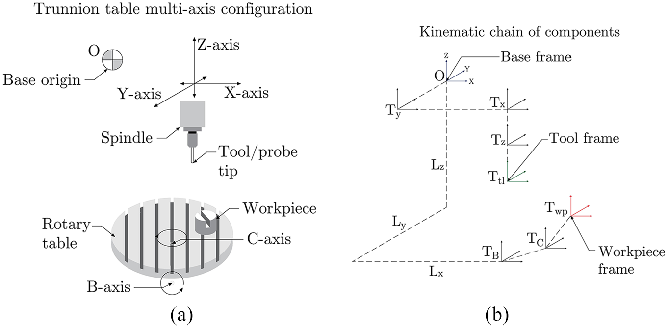
Configuration of kinematic components in multi-axis machine tool investigated in this paper: (a) physical components of the kinematic chain, with BC rotary table and XYZ linear-axes on the tool side and (b) relative coordinate systems in the kinematic chain.
Five more parameters define the position and orientation errors of the axis average line, defined in ISO230-7 as ‘a straight line segment located with respect to the reference coordinate axes representing the mean location of the axis of rotation’. These parameters – also known as the axis shift, or location errors– comprise two positional errors, two orientation errors and one zero position error. Again, for the B-axis, these are (
Geometric error parameters of BC-configured rotary-axes.
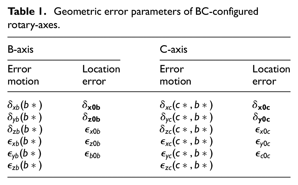
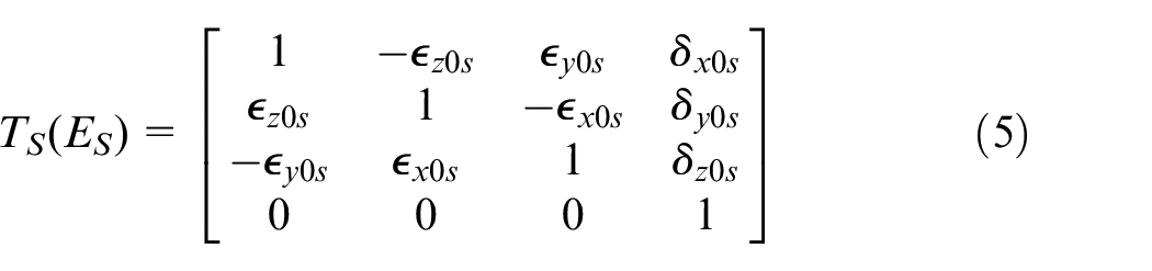
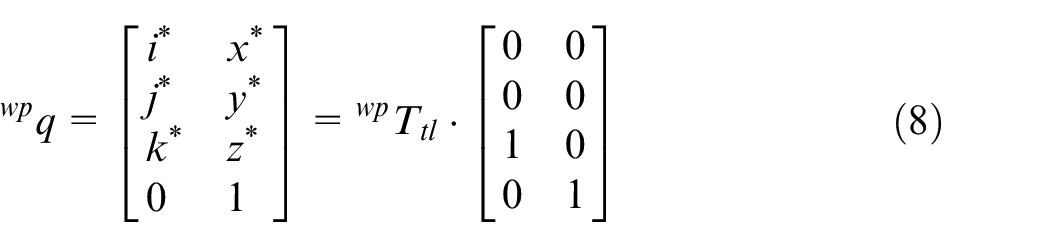
A necessary feature in a multi-axis machine tool controller is the ability to define the pivot point of the rotary-axes within the machine coordinate system. As a result of this, correcting the positional location errors (
The positional location errors, described above, are the ones most at-risk of mis-management, if proper care is not taken when utilising two or more different multi-axis positioning functions on the same machine tool and workpiece. In order to demonstrate this experimentally, the succeeding sections will assume negligible effects of error in the linear-axes. In evaluating each function, measurement data were obtained for identical rotary-axis indexations, such that the effect of linear-axis errors during comparison will be negligible-to-nil. As will be detailed in Section 2.3, the critical factor which can cause problems is the setting of the pivot point, which is solely influenced by the positional errors. For the comparison, it is beneficial to omit the orientation and zero position errors; these are not as easily corrected, and as such, are not subject to the same risk of mis-management as the positional errors are. This is achieved in the methodology by intentionally inflating the positional errors to very large values, causing any present orientation errors to be negligibly-small by comparison.
Kinematic model of the multi-axis machine tool
The key physical components of the multi-axis machine tool considered for this paper are illustrated in Figure 1(a). Movement in the X-, Y- and Z-axes is achieved through three linear guideways on the tool side of the base origin, with a bridge configuration for the X- and Y-axes, and octagonal ram construction for the Z-axis, 17 providing high thermal and structural rigidity. Rotation is performed in the B- and C-axes (about the Y- and Z-axes, respectively) through a trunnion-style rotary table on the workpiece side.
The general objective in NC programming is to accurately drive the tool tip around the workpiece, facilitating material removal and subsequently controlled geometry creation. This is most commonly and easily achieved by defining an origin on the workpiece, and using knowledge of the machine tool’s kinematics to calculate the required tool tip positions for each command.
Defining the base frame, O, located at the origin illustrated in Figure 1(b), the tool, tl, and workpiece, wp, frames are formed as branches from O. The relative position of tl to wp can be obtained by,

where
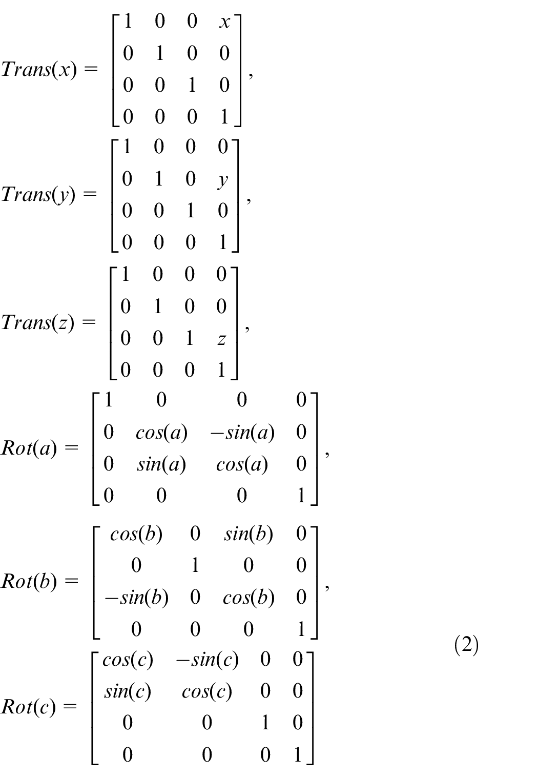
the general transformation from one frame to its predecessor can be represented by the combination of all translations and rotations,

for linear displacements

where
where


The origin of the workpiece frame is generally referred to as the work offset. The location of the work offset is unique to every setup, but is included as a nominal offset in the transformation
This derivation describes the forward kinematics of the multi-axis machine tool, which provides sufficient context for this paper. The derivation can be extended to calculate the physical axis positions that correlate commanded tool tip positions, relative to the workpiece frame, which are obtained by solving the inverse kinematics of the system. In the HTM approach, the inverse kinematics solution is implicit, obtainable by either an iterative numerical approach, or analytically by a closed form solution. 21 An alternative approach, which has become increasingly popular in the literature, is to apply screw theory to model the multi-axis kinematics,22,23 which provides an explicit solution to the inverse kinematics.
Numerical control programming approaches
It is possible to produce NC-code to calculate tool position in a multi-axis operation, according to the mathematical method – or similar method 24 – described in Section 2.2. In this, as the equations required for kinematic transformation are built into a software subroutine called a Postprocessor. The Postprocessor is a unique driver, specific to each machine tool, which takes generic toolpath data from Computer-Aided Design/Manufacturing (CAD/CAM) software and converts it into machine-readable NC code. This includes the general definition of NC-code functions – for example, functions written for a Fanuc controller will not work on a Siemens controller, and vice versa – as well as machine kinematics, necessary modal commands (e.g. defining programming in mm or inches, absolute or incremental positioning, etc.) and any customised alterations to ensure operations are conducted effectively.
In practice, compensating for kinematic error in the Postprocessor directly can lead to considerable operational inefficiency. As the nature of kinematic error is variable, it is important to take the current error state into account when calculating tool position to ensure accurate workpiece production. Based on individual requirements, it is possible that a single workpiece may be assigned to multiple machine tool for production; conversely, a single machine tool might be used to produce many different designs. Managing kinematics in the Postprocessor is problematic in both cases; particularly the former, which necessitates unique versions for each machine tool, but in both cases there is a requirement to ensure kinematic errors are accurately measured and all programs re-processed after every instance of maintenance. This traditional approach does still occur at some facilities, although the convenience of modern controllers and high risk of issues is making it more and more a relic of the past. Nowadays, it is more common to straightforwardly manage the errors in the controller, allowing the use of advanced multi-axis positioning functions with attributes designed to improve process performance and programming.
Direct pivot point
As described above, the kinematic model can be defined in the Postprocessor, and utilised this to calculate the tool tip position given a particular multi-axis command. For this approach, denoted in this work as Direct Pivot Point (DPP), it will be presumed that only kinematic motion is calculated in the Postprocessor, and errors are managed on the controller itself. This is more reflective of a modern production approach, which might be found on a typical shop floor environment employing this technique nowadays. The errors, in this case, are managed in the work offset register G54. G54 stores the location of the rotary table pivot point, and all programming is conducted directly with this location as the origin. Figure 2(a) illustrates a simple positioning example with the corresponding NC-code blocks. Equations (6) and (7) can be modified to describe the DPP approach by,
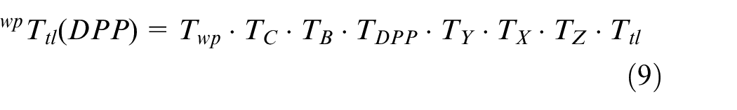
where
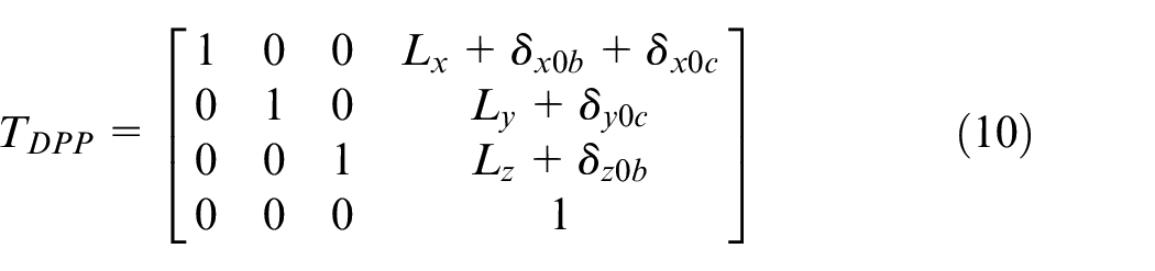
The programming frame is fixed at the pivot point by the nominal offset,
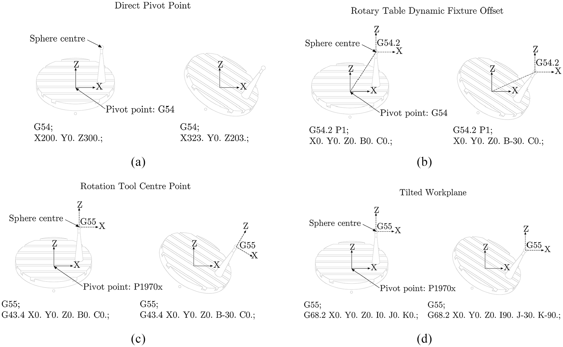
Frame handling with the four controller functions investigated in this work. Each subfigure shows a spherical artefact mounted on a rotary table, at the home position (B- and C-axes both at zero, left) and at a minus-thirty degree pivot of the B-axis (right). Below each diagram is an example NC-code block which defines the sphere centre location in each programming approach: (a) multi-axis programming directly from the pivot point (DPP), defined here at G54. Note that the programming frame remains fixed to the pivot point, and the new sphere centre position is calculated in the XYZ coordinates, (b) RTDFO programming, incorporating an offset from the programming frame (G54 pivot point) to the true workpiece frame. RTDFO is commanded here with G54.2; the programming frame origin is shifted to the sphere centre via the recorded location of G54, maintaining the frame orientation in parallel with the tool/base frames, (c) RTCP programming, with the rotation centre located at the tool tip. RTCP is commanded here with G43.4; this time, a new work offset is recorded for the sphere centre in G55, which is dynamically repositioned during table rotation. Note that the orientation of the frame is also reoriented with rotation, such that it always remains parallel to the table, and (d) tilted workplane programming, for 3 + 2-axis machining. TW is commanded here with G68.2, which involves defining a new origin on some part of the workpiece in XYZ and an IJK vector defining the desired rotation angle; the frame orientation remains parallel to the tool/base frames.
Rotary table dynamic fixture offset
Interpretation of commanded tool positions, and simplification in programming, is greatly improved through the use of a specific multi-axis positioning function. As for DPP, Rotary Table Dynamic Fixture Offset (RTDFO) utilises the G54 work offset at the pivot point, but incorporates an additional offset (G54.2) to define the true workpiece frame with an origin on the workpiece itself. All kinematics are calculated within the RTDFO function which makes programming more straightforward than the DPP approach. The resultant NC-code is also easier for the operator to interpret – tool positions are defined relative to the workpiece offset, with the axis motions described in the code conveniently aligned with the base machine coordinate system orientation. RTDFO can be interpreted in the kinematic model with the addition of a programming frame,

where
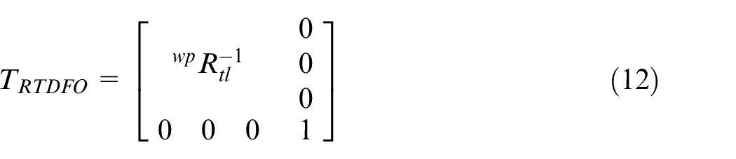
and
Rotation tool centre point
An alternative approach for dynamically controlling multi-axis motion is Rotation Tool Centre Point (RTCP). The RTCP approach effectively shifts the centre of rotation to the tool tip, re-orientating the machine kinematics and subsequently the workpiece, around that point in real time. As a result, both the origin location and orientation of the workpiece frame remain fixed to the workpiece throughout multi-axis motion, illustrated in Figure 2(c). Interpretation of RTCP in the kinematic model is straightforward, with,

where the transformation to the programming frame,
Similarly to RTDFO, RTCP is ideally suited to producing curved and free-form geometries. The key difference, however, is that the RTCP approach references a different set of offsets for calculating positioning with consideration to kinematic error. These are lockable parameters in the controller’s system settings, as opposed to the previous two approaches which rely on managing offsets in the work offset user interface. P1970x will be used henceforth to reference this parameter set, reflecting their location on a Fanuc-based system, as considered in this paper. The errors are defined separately for each axis, providing a total of six positional error parameters for the two rotational axes. Unlike the G54 approach, these error parameters are introduced separately to the kinematic model, such that the positional errors associated with the B-axis are included in
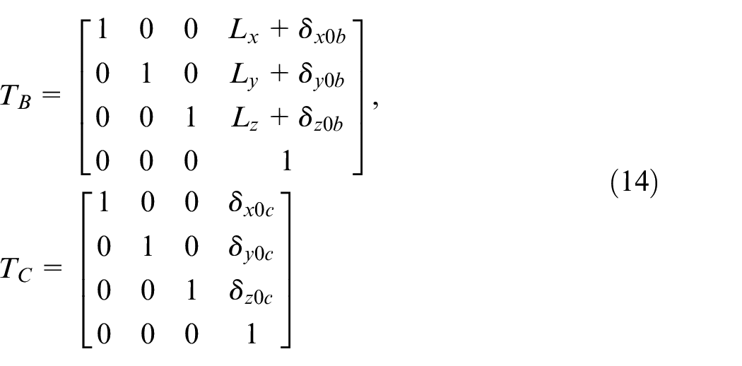
Note the addition of positional errors normal to the axis of rotation,
Of the three specialist controller functions considered in this paper, the RTCP function has appeared in the literature most frequently. The concept of a measurement coordinate system fixed to the workpiece frame was utilised to develop an alternative and simplified geometric error model for rotary table-based machine tools, 25 based on the traditional forward/inverse kinematics method. More recently, the corrections applied by dynamic approaches (both RTCP and RTDFO) during motion to maintain a constant relative distance between the tool and workpiece have been incorporated into error modelling strategies, integrating RTCP into a traditional geometric error compensation approach 26 and for detecting linkage performance through the evaluation of RTCP trajectories. 27
Tilted workplane
Unlike the dynamic orientation applied with RTCP and RTDFO, the Tilted Workplane (TW) command is a method of statically reorienting a workpiece to machine simple features but at non-orthogonal angles. It is a popular approach in industry, and is colloquially referred to as 3 + 2-axis machining, due to the fact that the (two) rotary-axes initially move to a specified orientation, then the linear-axes perform a three-axis operation at that new rotation, as is illustrated in Figure 2(d). Simultaneous motion of the linear and rotary-axes is not permitted in a TW operation. The TW function references the P1970x parameters, in the same manner as RTCP.
TW can be commanded by defining a set of Euler angles which describe the desired orientation of the feature programming frame. A translational offset,
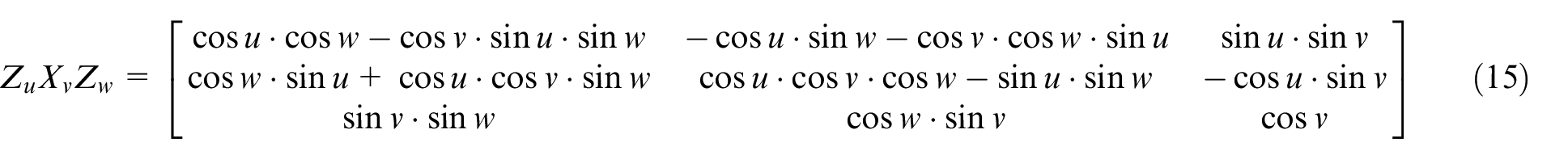
where
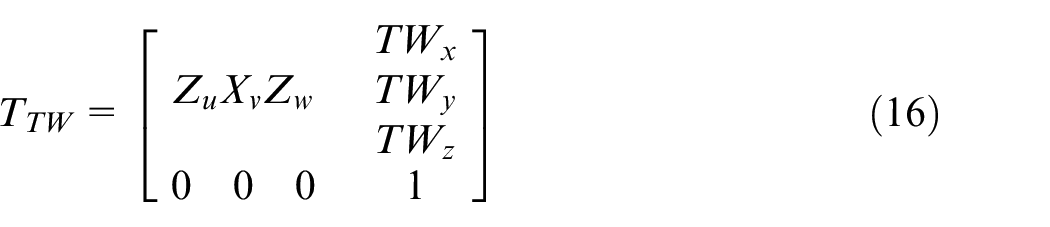
and finally,

Similarly to RTDFO, the Z-axis of the programming frame in TW is always parallel with the tool axis, ultimately defining the physical axis positions that can be determined through the inverse kinematics solution.
Although each method handles programming frame origins and orientations differently, the critical issue, raised in this paper, is the way they incorporate knowledge of positional errors. If various approaches for multi-axis positioning are to be applied – such as free-form machining with RTDFO and static reorientation with TW – in a machining strategy, it is imperative that the positional error parameters described in equations (10) and (14) match exactly, and both storage locations contain up-to-date values. Neglecting to update the errors in both locations during a calibration routine can have severe consequences on workpiece accuracy, and such an oversight is not unrealistic in a busy shop floor environment. The following section now describes the methodology employed to demonstrate such effects, by leveraging the theory in this section for a simulation-based approach and experimental validation on a real production system.
Methodology
Simulation
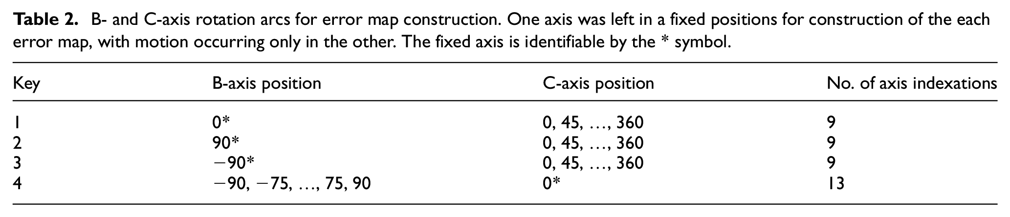
A mathematical simulation was produced with the HTM approach, described in Section 2, to demonstrate the expected differences of the G54 and P1970x error parameter storage locations. The kinematic model was evaluated to calculate the expected error at each rotary-axis indexation detailed in Table 2, taking the positional errors in 3 and 4 as kinematic model parameters. The expected errors at each indexed position were then arranged according to Table 2 simulating a total of four rotary-axis error maps.
B- and C-axis rotation arcs for error map construction. One axis was left in a fixed positions for construction of the each error map, with motion occurring only in the other. The fixed axis is identifiable by the * symbol.
In order to reliably compare the programming functions, it is important to maintain nominally-identical machine conditions between the respective tests. As a result of this requirement, it is viable to make a number of assumptions to simplify the expressions (5) and (6) defined in Section 2 for the simulation. As the machine tool utilised for testing each function is constant, the nominal positions and orientations of each link in the kinematic chain are also constant and, as such, are irrelevant to the comparison. Thus, all

for the approaches that capture errors in a G54 work offset and,

for the approaches that capture errors in the P1970x parameter tables. Note that the critical difference between equations (18) and (19) is the point in the kinematic chain in which each error parameter set are considered. For G54 work offset-based approaches, the parameters in both
Experimental
An experiment was designed to demonstrate the potential differences in identifiable error when running identical axis checks in different NC-programming modes, based on the static test procedure detailed in Section 6 of ISO230-7. 2 A calibrated, spherical artefact was positioned centrally in a machine tool with a BC-configured rotary table, as illustrated in Figure 3(a). A touch-trigger probe was then utilised to locate the sphere at each rotary-axis indexation, taking a total of nine measurements on the sphere surface to calculate the centre point. The initial performance of the probe was determined prior to conducting the experiment, and the results are shown in Table 3.
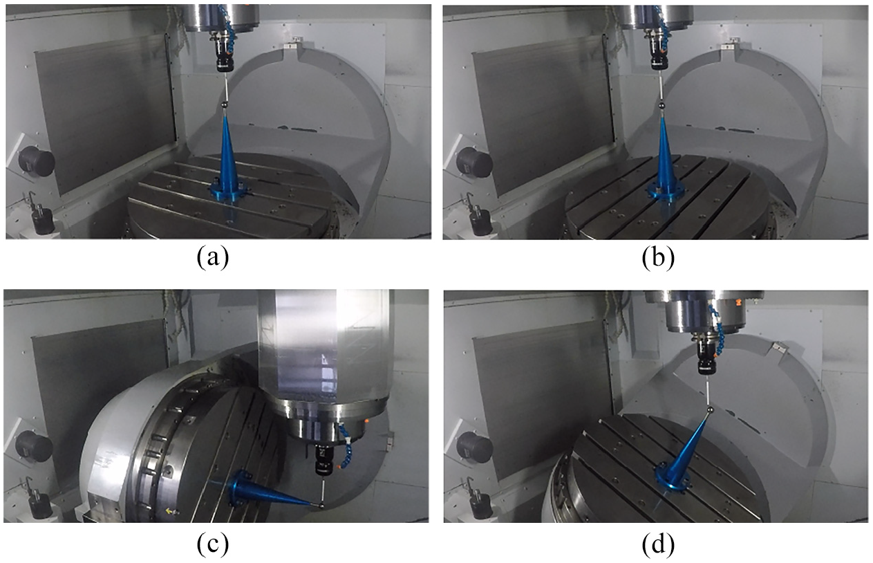
Experimental setup and example rotary-axis indexations for constructing the error maps in this study: (a) rotary-axes indexed at the ‘home’ position, B =
Probe calibration and repeatability results obtained immediately prior to the experiment.
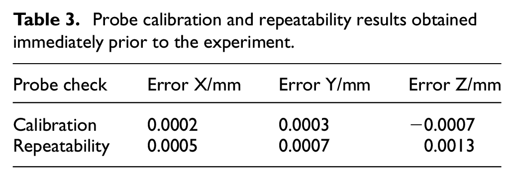
Calibration quantifies the performance of the probe to accurately collect measurements, with values automatically compensated-for in the results presented in Section 4. Repeatability tests the probe’s precision across multiple identical measurements. The results of these test were excellent, in a range of 0.2–1.3
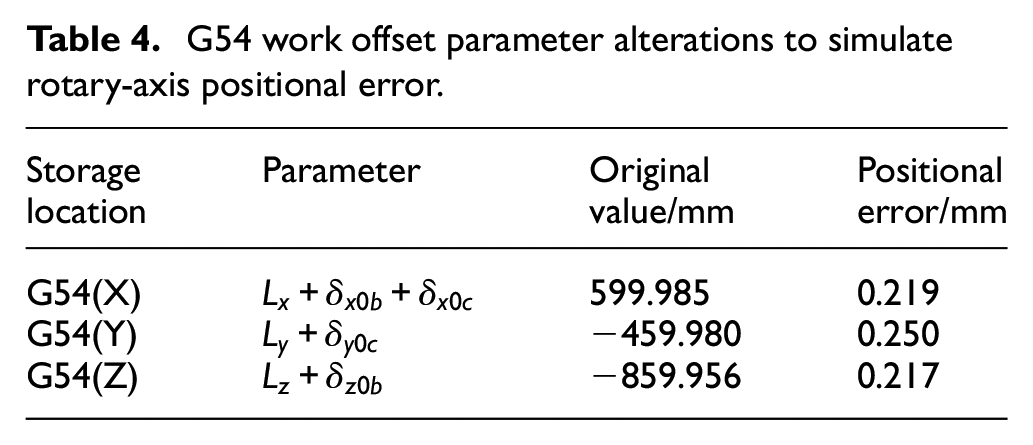
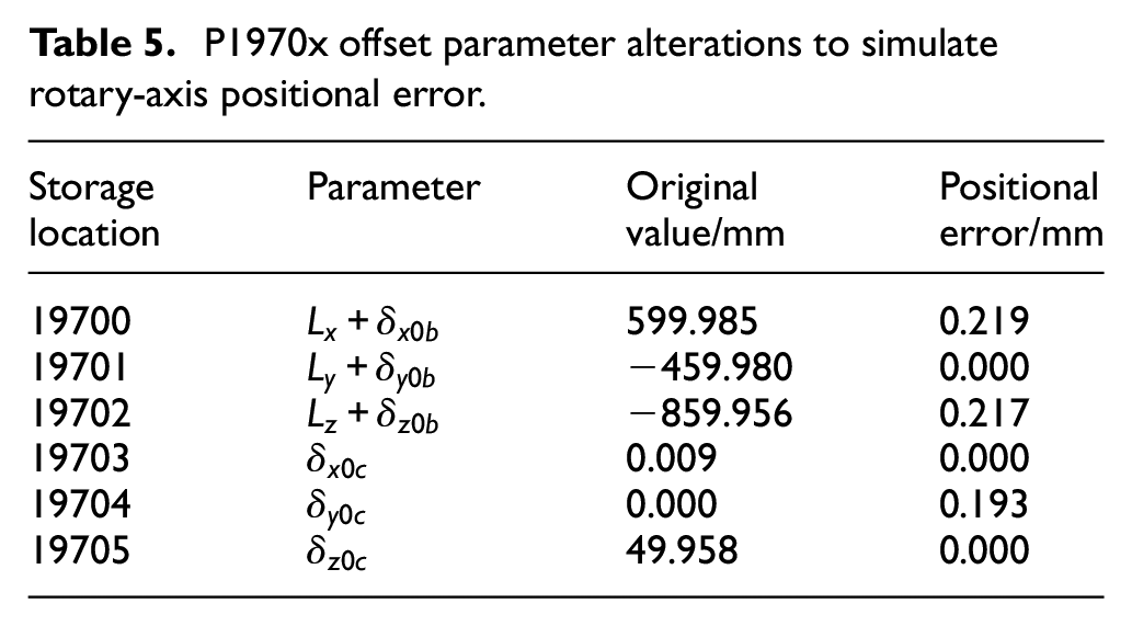
Pivot point positional error compensation values held within the controller were adjusted as detailed in Tables 4 and 5. The deviation values were determined to approximate a 250
G54 work offset parameter alterations to simulate rotary-axis positional error.
P1970x offset parameter alterations to simulate rotary-axis positional error.
Error maps were then collected for each of the four programming approaches at various axis positions, given in Table 2 alongside an identifier key for each map and the number of points collected. Figure 3(b) to (d) show the artefact at various rotary-axis positions indexed for data collection, as visual examples of the procedure. The results at each indexation were converted from a three-dimensional coordinate vector to a Euclidian distance, describing the extent of measurement’s deviation from the average error measured across the map. As the programming approaches in this paper each handle frame orientations in unique ways, these steps are important to ensure comparability in the results. Ultimately, it is the size and shape of the error map which one wishes to compare, however extraneous errors – such as an inaccuracy in the tool length setting – and the frame which each measurement is reported in impacts the position and orientation of the error map, when observed in the probing procedure’s reporting space. Normalising the error map values about their collective average ensures that the map is positioned centrally in the reporting space, irrespective of the frame orientation in which the data was collected. Converting the error map coordinates to Euclidian distances then removes the impact of varying orientation in the reporting space, which provides a reliable and generalised metric to compare results between the respective programming approaches. An LSE was also performed on the data to estimate the positional error parameters on the machine, as measured by each probing procedure. The results are presented for comparison in Section 4.
Results
The results from the probing trials described in Section 3 are presented herein. A true radial error – that is, radial error alone, with negligible influence from any other error source in the kinematics – is observable by smooth, circular plots in the plane that is perpendicular to the axis of rotation, with a nominally flat profile in the other two planes.
Figure 4(a) shows the theoretical expectation of the differences between G54- and P1970x-based approaches, based on the kinematic modelling approach described in Section 2, and equations (18) and (19). Figure 4(b) presents the results of each error map collected through on-machine probing, as the Euclidian distance from the error map’s average value.
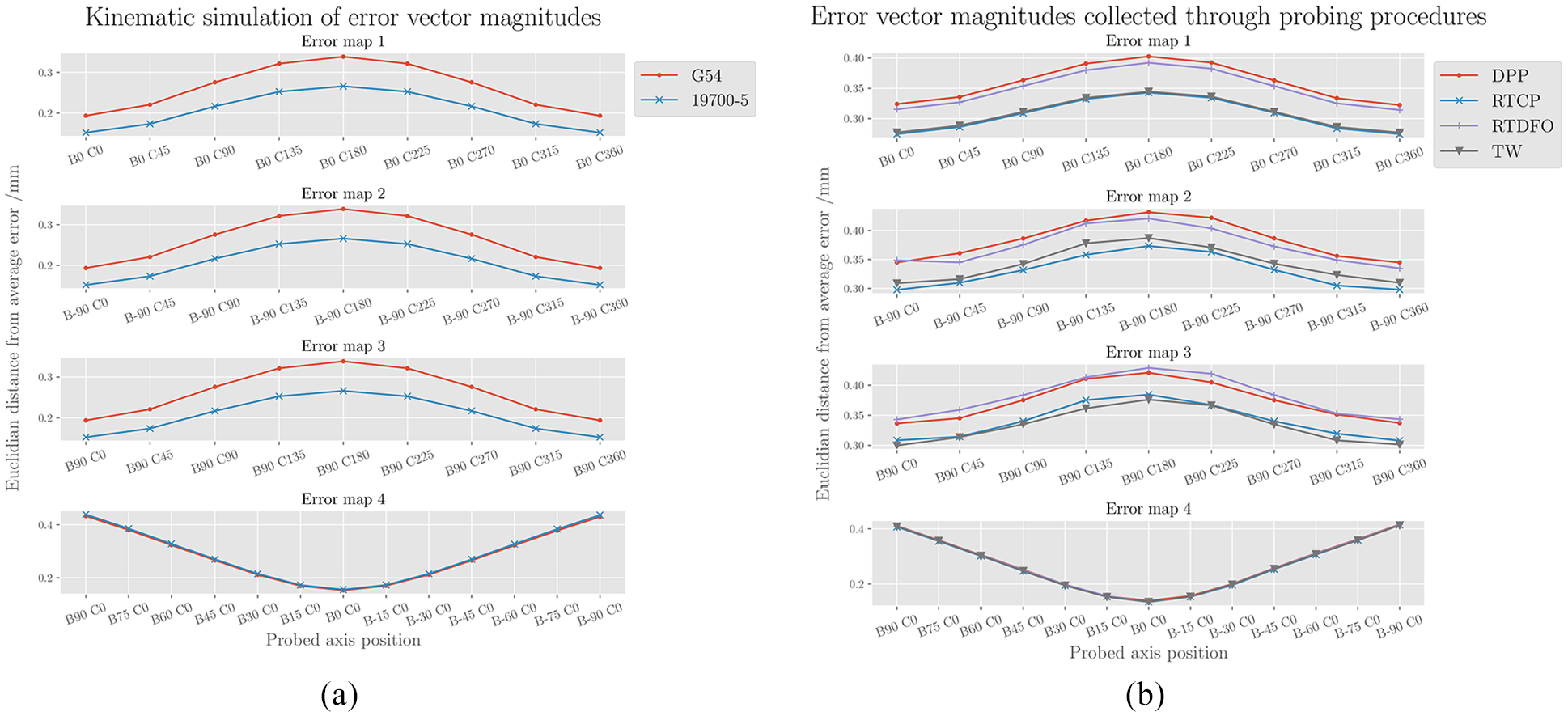
Comparison of methods across error maps, as Euclidian distance from the average error per approach: (a) kinematic simulation results and (b) on-machine measurement procedure results.
The simulation results for error maps 1–3 clearly demonstrate the effects of mismatched pivot point parameters, with the G54-based approach reporting larger error vector magnitudes than the P1970x approach, consistent with the mismatched parameter values in Tables 4 and 5. The probing results in Figure 4(b) are in agreement with the simulation, with the measurements of the G54 (DPP, RTDFO) and P1970x approaches (RTCP, TW) reflecting the corresponding simulation trends well. Error map 1 – where the B-axis was fixed, and only the C-axis indexed – exhibits the most consistent measurements between DPP/RTDFO and RTCP/TW. For error maps 2 and 3, there is a little more deviation, although they still demonstrate a clear correlation with the expected results due to the mismatched positional error parameters. As both maps were collected with the table positioned at a
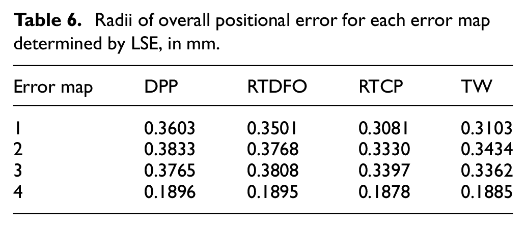
Table 6 shows the values obtained with an LSE for the four error maps collected for each programming approach. Figure 5(a) to (d) present these values visually, as the eccentric circle which would be produced by the given error.
Radii of overall positional error for each error map determined by LSE, in mm.
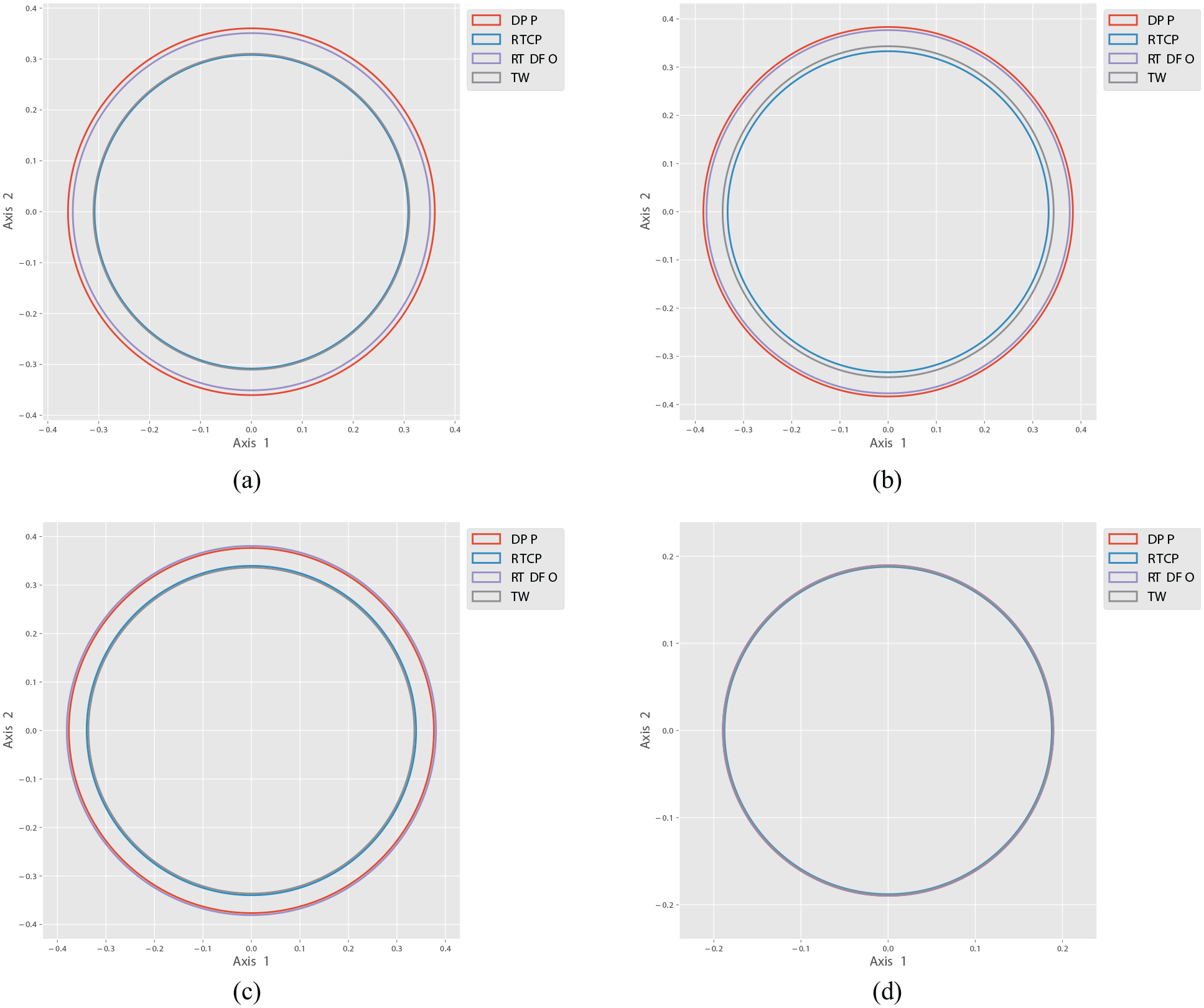
Expected positional error, through LSE fit on various error maps: (a) LSE positional error for error map one, (b) LSE positional error for error map two, (c) LSE positional error for error map three, and (d) LSE positional error for error map four.
Generally, the relationships between the two offset storage locations – G54 for DPP and RTDFO, and P1970x for RTCP and TW – are clearly observable in the data presented in Table 6. There is a clear distinction between the two groups, with G54-based approaches consistently returning higher values, due to the larger positional error induced in the Y-axis, as defined in Tables 4 and 5.
Specifically, for error map one, the two expected groupings are again clear, with a maximum difference of 50.2
Concluding remarks
The results, presented in Section 4, clearly demonstrate that a mis-match in the pivot point parameters between the two possible locations can readily lead to unexpected errors in the finished workpiece. With a proper understanding of the way these parameters are stored, this conclusion is intuitive; however, it is a real issue affecting some parts of the industry 29 which must be definitively stated. Error parameters pertaining to the pivot point of the rotary-axes must always be managed in both locations, to ensure accurate workpiece production irrespective of the chosen multi-axis positioning function. Methods which rely on the work offset register G54 to store these offsets are more at-risk than those which apply offsets from parameters P1970x, as it is much easier to mistakenly edit the offset in G54 during standard, day-to-day operation. As such, this paper would primarily recommend using the RTCP or TW programming approaches, as compared with DPP or RTDFO; that said, consistently using the same function or at least being aware of the issues will greatly reduce the likelihood of introducing unexpected errors in this manner.
The experiment conducted for this paper focuses on a Fanuc-type machine controller, however the recommendations of careful pivot point management should be adhered to in any system. Generally, any approach which handles the kinematics in the postprocessor (DPP), or otherwise directly references the pivot point with a work offset (RTDFO), runs a risk of mismatch when used in conjunction with specific controller functions for multi-axis positioning. Alternative controllers have different functions; however, there are often similarities in their general approaches. For example, the Siemens SINUMERIK control system performs full five-axis machining (RTCP) with a function called TRAORI, and 3 + 2-axis machining (TW) with CYCLE800. For a Heidenhain TNC controller, the functions are PLANE and M128, respectively. For both systems, the pivot points are stored in a parameter set synonymous with the Fanuc P1970x location, but the implementations vary due to differences in the systems and developers. Future work should consider repeating the experiment on alternative control systems, to verify that the findings of this paper translate universally to all types of machine tool controller.
Footnotes
Appendix
Declaration of conflicting interests
The author(s) declared no potential conflicts of interest with respect to the research, authorship, and/or publication of this article.
Funding
The author(s) disclosed receipt of the following financial support for the research, authorship, and/or publication of this article: The authors would like to gratefully acknowledge Metrology Software Products Ltd. and the Engineering and Physical Sciences Research Council (EPSRC) grant EP/I01800X/1 for supporting this research. KW would like to additionally acknowledge support from an EPSRC Established Career Fellowship EP/R003645/1.