
Abstract
Maintaining high levels of geometric accuracy in five-axis machining centres is of critical importance to many industries and applications. Numerous methods for error identification have been developed in both the academic and industrial fields; one commonly-applied technique is artefact probing, which can reveal inherent system errors at minimal cost and does not require high skill levels to perform. The primary focus of popular commercial solutions is on confirming machine capability to produce accurate workpieces, with the potential for short-term trend analysis and fault diagnosis through interpretation of the results by an experienced user. This paper considers expanding the artefact probing method into a performance monitoring system, benefitting both the onsite Maintenance Engineer and visiting specialist Engineer with accessibility of information and more effective means to form insight. A technique for constructing a data-driven tolerance threshold is introduced, describing the normal operating condition and helping protect against unwarranted settings induced by human error. A multifunctional graphical element is developed to present the data trends with tolerance threshold integration to maintain relevant performance context, and an automated event detector to highlight areas of interest or concern. The methods were developed on a simulated, demonstration dataset; then applied without modification to three case studies on data acquired from currently operating industrial machining centres to verify the methods. The data-driven tolerance threshold and event detector methods were shown to be effective at their respective tasks, and the merits of the multifunctional graphical display are presented and discussed.
Keywords
Introduction
To remain competitive in the modern advanced manufacturing sector, it is becoming increasingly important to embrace and implement intelligent systems for process monitoring. The core capability for data and analytics strived for in the Industry 4.0 movement 1 is a key motivator for this change. Information transparency, concerning the application of on-line data collection to facilitate analysis of the physical system, is a particularly attractive topic for research and development, and applying machine learning paradigms to physical engineering processes presents itself as an effective solution to the problem. The resultant output should then be informative in providing technical assistance to the Manufacturing or Maintenance Engineer (ME), fulfilling two of the four design principles set out for Industry 4.0. 2
It is not possible to consistently manufacture with absolute accuracy and precision; there will always be some observable, quantifiable degree of error present on a manufactured workpiece, as compared with its idealised specification. However, communication through the Geometric Dimensioning and Tolerancing system 3 allows realistic manufacturing of any reasonable engineering design. Variation in quasi-static and dynamic error sources 4 that affect machining accuracy arise due to local temperature fluctuations, in-process conditions, significant events (such as a tool crash, or calibration activity), errors in the size and form of machining centre components as well as general wear of moving elements throughout normal operation. The extent, effect and complexity of compounding error is unique to any particular machining centre and its life cycle, leading to the possibility that two otherwise identical systems may exhibit significant performance differences in their production output. It follows that the performance of a unique system will tend to drift over time, 5 as its compound error profile is affected through further operational use. A requirement for repeatable performance in the manufacturing process has led to the development of error identification methods for informing machine calibration cycles, or qualification to operate by assessment of machine capability.
Accordingly, much research in recent years has been dedicated to the accurate identification of the parameters which mathematically define the kinematic error motions, with particular interest in the variable location errors, to inform necessary maintenance actions such as calibration or specific repairs. A prominent example of this is the R-Test, 6 which is currently recognised as an ISO standard 7 and has been shown to be effective for multi-axis machine tool calibration. 8 The original method used three linear displacement sensors to dynamically track the location of a calibrated, spherical artefact through ranges of motion in the rotary axes. An example of recent commercialisation 9 of the technique employs a non-contact 3-D probe based on eddy currents to the same effect. The procedure results in a detailed error map which can be used to diagnose machine faults (kinematic eccentricity, misaligned axes, backlash etc.) and inform a calibration action. Static variants of the R-Test, where the procedure and equipment setup is replicated but data are collected at discrete intervals, have been applied for complete error map construction of all location errors and the larger class of position-dependent geometric errors. 10
The R-Test is a fast 9 and reliable method for kinematic error identification in machine tool rotary axes, but it has the drawback of requiring specialist equipment to conduct. A common alternative is to use a touch-trigger probe to inspect an artefact of precisely known dimension, in a procedurally similar manner to the static R-Test. Calibrated artefact probing is attractive to many in the industry due to the ubiquitous nature of the touch-trigger probe, used in virtually all modern facilities for pre-machining verification, fault diagnosis and calibration. The main trade-off for this minimised cost is the overall speed of the procedure, as multiple contact points on the artefact must be probed to precisely determine its location, as compared with the R-Test which requires only one contact per rotary-axis position. An approach involving probing a rectangular artefact across numerous probing patterns 11 has been shown to be effective for rotary-axis location error calibration. This work was then extended to construct a complete error map by artefact probing, to much the same effect as the static R-Test publication noted above. 12 Spherical artefacts are often favourable, due to their nominally-identical form when approached from different angles. The artefact is probed numerous times and spherical interpolation applied to determine its true centre point, resulting in an informative error map which can be applied in much the same way as its dynamic counterpart. The scale and master balls artefact method 13 employs touch-trigger probing to locate a collection of precision balls at various axis positions, and has been shown to provide sufficient data to estimate all axis-to-axis location errors in a five-axis machining centre. More recently, the method has been applied for kinematic fault diagnosis. 14
The core focus with artefact probing procedures and commercial software is error identification for machine capability checking or calibration activities. Generally speaking, performance monitoring and fault diagnosis in machine tools are of interest to the community; recent research has considered the mining of general in-process data across networks of machining centres, 15 analysing the energy usage to detect abnormalities 16 or vibration response to assess the health of the axis drives. 17 Monitoring machine performance with artefact probing data is also possible as a secondary application; however, it is often overlooked, and as such, effective systems for interrogating legacy data have not been developed. Such a system could be of great benefit to both the onsite ME and visiting specialist consultants, enabling them to quickly and easily interpret legacy data and extract critical insight on the machine’s history, usage and signature. Developing a performance monitoring system like this also presents the opportunity to employ novel predictive modelling techniques, introducing intelligent features and automation to further assist the user.
The paper is structured as follows. Firstly, the experimental procedure for artefact probing is described, as well as the data post-processing and presentation currently employed for performance monitoring purposes within a popular commercial solution. 18 The analytical methods proposed for the monitoring system are then presented; including a tutorial for interrogating the results on a simulated, demonstration dataset, and a visual comparison of the kernel options to select the most appropriate. Then, three case studies are evaluated, applying the methods to real datasets acquired from the manufacturing industry. Finally, concluding remarks and a discussion on the proposed system are presented, with consideration of further research on the topic.
Experimental procedure
The probing procedure, which this paper aims to develop, involves locating a single, spherical artefact at numerous indexations of the rotary axes. Generally speaking, the Primary-axis of a machine tool is defined as the C-axis, and the Secondary-axis is either the A- or the B-axis, dependent upon the specific configuration. For this paper, a B-C machine tool configuration will be considered. The method has a number of similarities with a recent paper,
19
which proposed a Least-Squares Estimation approach to identify and calibrate rotary-axis location errors. A calibrated, spherical artefact is firstly located at the ‘home’ position, where the rotary axes are indexed at B=
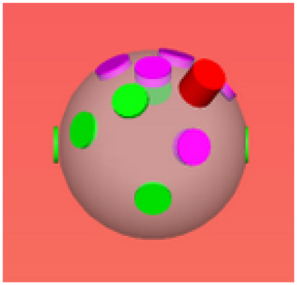
Visualisation of points probed on the sphere surface for a typical indexation. 18 The height of the extrusions indicate the extent of the error identified at each point on the surface.
At the home position, it is possible to run a number of checks to quantify the performance of the probe itself. This includes assessing the axial pre-travel (the distance traveled before the probe is triggered), the repeatability of the automatic tool change action or characterising the overall performance. The artefact is then reoriented relative to the probe, incrementally, along specified arcs of rotation to determine the performance of the rotary-axes.
Figure 2(a) shows the typical setup, with the rotary axes indexed at the home position; Figure 3 shows this in a diagrammatic format. The Primary-axis procedure described in this paper locates the sphere at thirteen indexed positions from C=
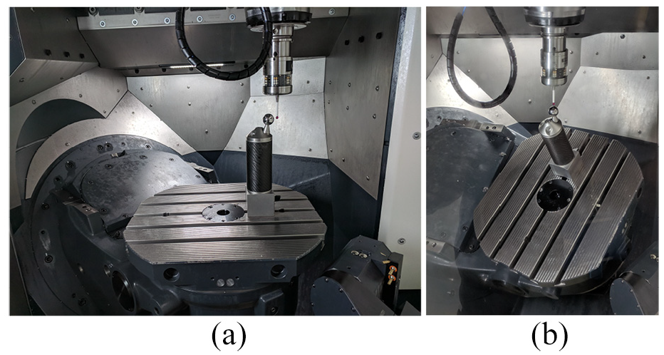
Hardware setup for performing the artefact probing procedure: (a) Probing the sphere at the home position and(b) Probing the sphere at an indexation of the Secondary-axis.
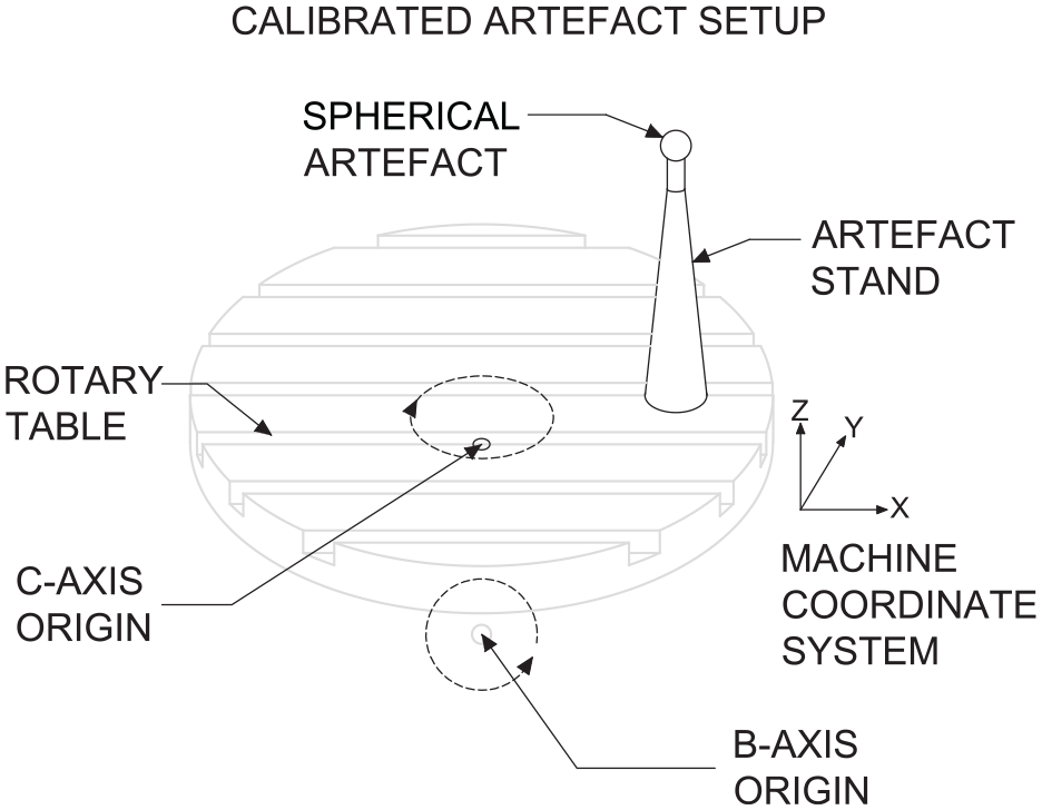
Diagram of typical spherical artefact setup on a B-C configured rotary table.
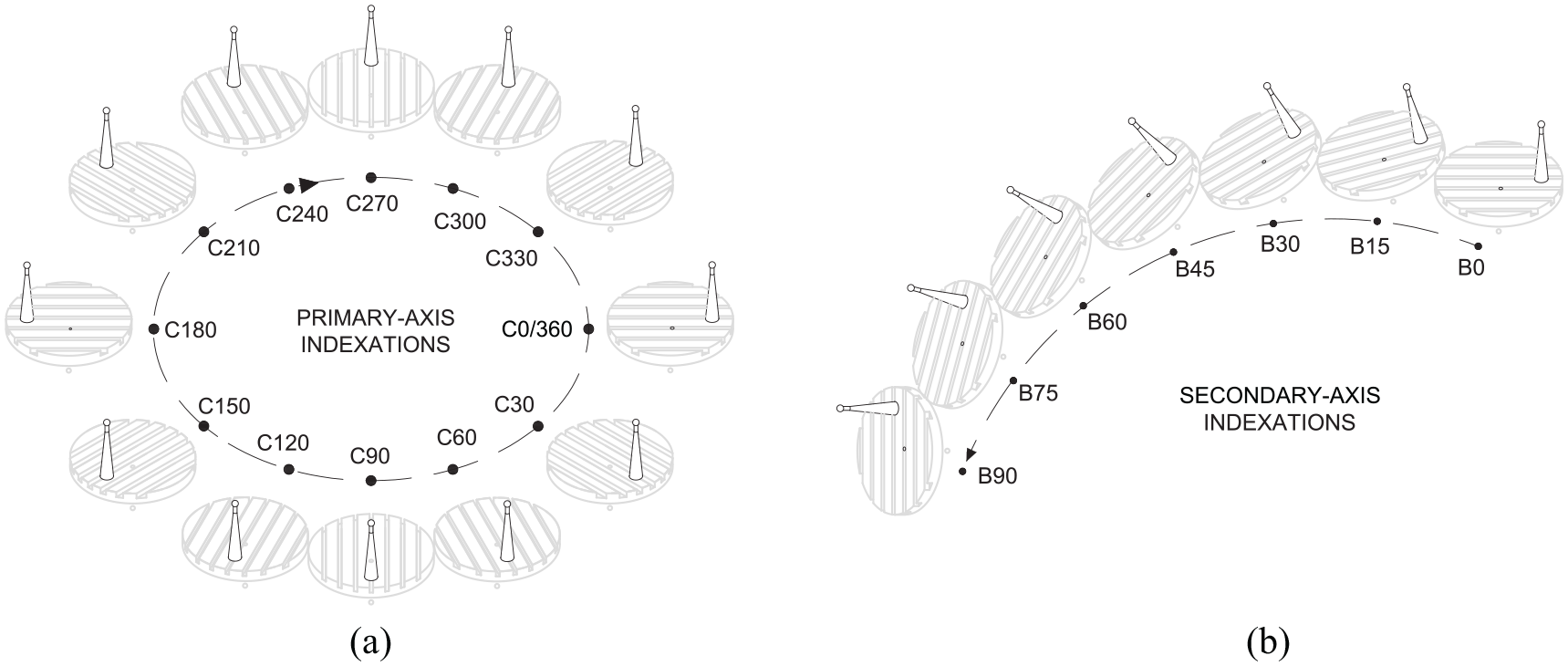
Indexations of the primary- and secondary-axes for the rotary-axis error identification procedures: (a) Typical rotary-axis positions for the Primary-axis procedure and (b) Typical rotary-axis positions for the Secondary-axis (+ve) procedure. The Secondary-axis (–ve) procedure is simply these indexations, but in reverse.
The intrinsic focus in machine capability is to ensure satisfactory part production in the short-term, implementing a green light manufacturing policy where operators can confidently and efficiently run machines without the need for high levels of additional, specialist skills. Proprietary software 18 achieves this by collating the data from a calibrated artefact probing procedure into a summary presentation – referred to as the benchmark performance and illustrated in Figure 5– and detailed reports for deeper analysis and fault diagnosis. Each spoke on the benchmark wheel represents a different test conducted by the software, such as Rotary Single Primary (a measure of the Primary-axis performance) or the Overall probe performance.
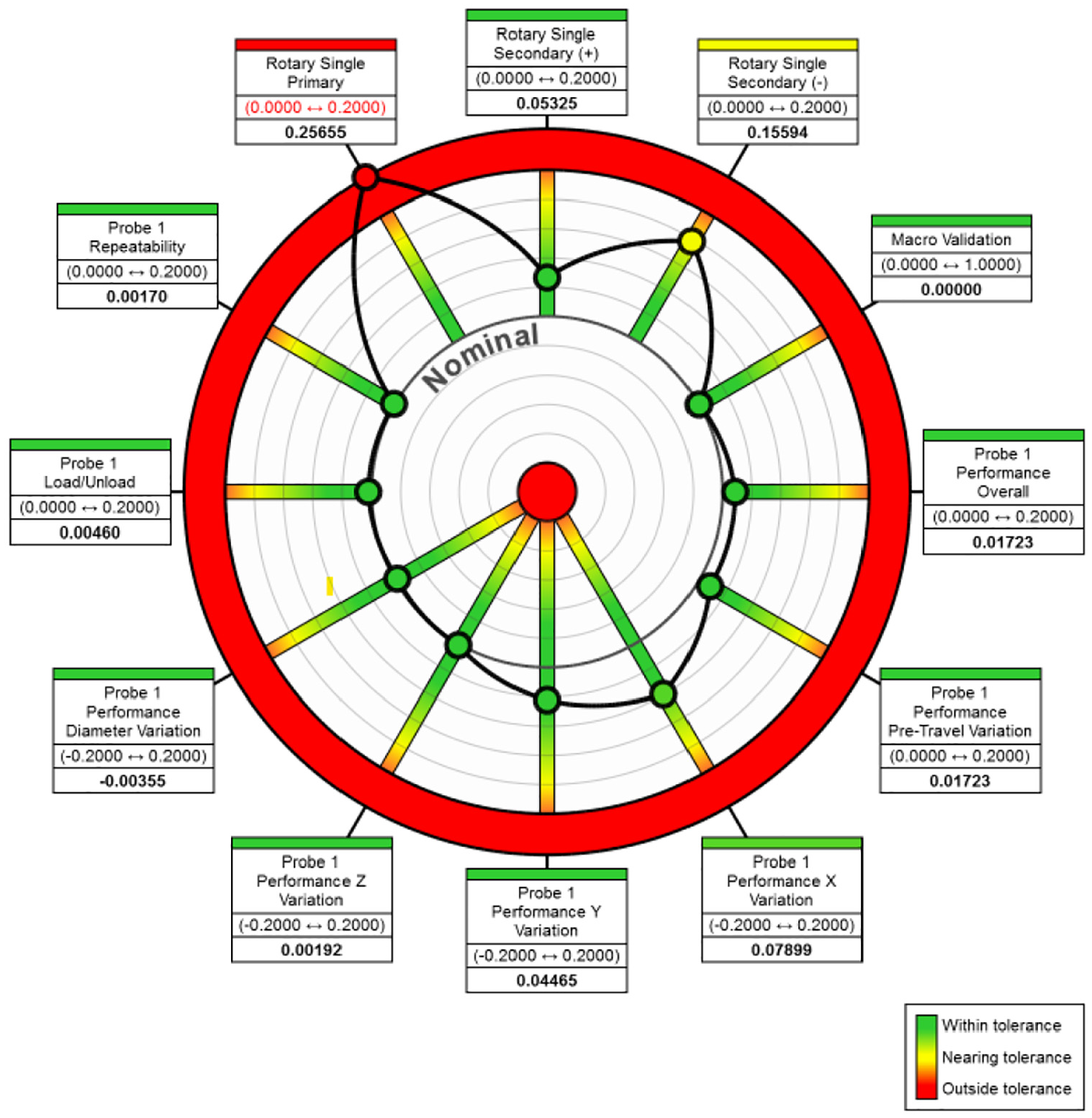
Benchmark performance summary, as produced by proprietary artefact probing software. 18
A foundational characteristic with the benchmark performance presentation is its ability to provide an instant appraisal of the system’s health state, which is accessible to personnel of all skill levels. In 1983, The Visual Display of Quantitative Information 20 by Edward Tufte was published, concerning the theory and practice of data graphics design. The benchmark performance presentation echoes many of the design practices set out by Tufte. The heavier line-weight afforded to the data elements helps establish contrast in meaning, as compared with the polar axis elements that have lesser graphical importance. Presented in this way, the data elements also serve as a multifunctional graphical element; every machining centre has its own unique signature, which is represented by the respective positions of each data element during normal operation. The signature is an important visual element for verifying that a group of machines producing the same part are likely to perform to similar levels. The inclusion of colour can often risk generating a graphical puzzle, in which the viewer is required to consciously decode the information presented before them. The benchmark presentation leverages colour effectively by implementing a red-yellow-green scheme, instantly recognisable due to the ubiquitous traffic light system in modern society.
Analytical methods
Learnable tolerance thresholds
A key decision-making process in capability checking concerns the proper setting of tolerance thresholds, which define the acceptable levels for each feature that characterise the machine’s error state. Thresholds are determined by the ME as a result of satisfactory feedback from the quality assurance process, generally depending on the production requirements and the industry for which they are intended. Incorporating normalisation with respect to the tolerance threshold is crucial for assigning meaning to the absolute error measurements obtained by the probing procedure. Reassignment of a machining centre to new production requirements may result in alterations to the tolerance thresholds. There is also the possibility of user error, or even intentional tampering, when setting new tolerance thresholds; this is to be avoided at all costs, and is an important motivator for incorporating learnable tolerance thresholds into any monitoring system with a foundation in geometric accuracy. Moreover, learning the most appropriate tolerance threshold from historical data is highly useful for representing the normal operating condition of any unique machining centre. This representation extends the potential for signature comparison, currently utilised in the benchmark capability checking system, to evaluate historical performance of a group of machines with respect to one-another.
In supervised learning, the core objective of a classifier is to produce a decision boundary separating two or more predetermined classes of data. It is likely that there exist numerous potential solutions for an appropriate decision boundary, so it would be wise to select the one which presents the minimal generalisation error. A Support Vector Machine (SVM) classifier attempts this by solving for the decision boundary which maximises the margin between the classes of data. 21 The SVM is a kernel method based on a sparse solution, such that new input predictions depend only on a relevant subset of the training data, known as the support vectors. The margin is defined as the smallest distance between the decision boundary and designated support vectors. Conveniently, the identification of model parameters corresponds to a convex optimisation problem, so any local solution can be considered a global optimum. 22
For a linearly-separable case, defined by kernel function,

the optimum decision boundary is determined by applying the constraint,

where
with parameter
A one-dimensional SVM (1D-SVM) approach is proposed to learn appropriate tolerance thresholds and inform future decisions. The artefact probing procedure considered in this paper is an off-line method, which necessitates a degree of disruption to the production process to conduct. Subsequently, the datasets obtained for use in a performance monitoring context are often relatively small. SVMs are generally better suited to tasks involving smaller datasets as compared with other predictive algorithms – the classic example being the artificial neural network, which requires extremely large training sets to properly mitigate the risks of overfitting - due to the fact that only a subset containing the support vectors are required to construct the hyperplane, irrespective of the total size of the training set. In fact, a critical drawback of the SVM is high computational costs for processing large datasets, with a common solution in recent research efforts concerned with extracting reduced training sets that are most likely to contain the support vectors. 24
Classes were assigned based on each measurement’s relationship with the engineer-determined tolerance threshold at the time, resulting in two classes; in-tolerance, and out-of-tolerance. The size of the dataset was increased by sampling each observation numerous times with additional Gaussian noise. This strategy ensured that the generalised model could be properly cross-validated (CV); it is possible that the data may contain only a single instance of one of the classes, causing the standard SVM algorithm
25
to fail, even with a Leave-One-Out CV scheme. Additionally, a number of points were introduced in the same manner close to 0.000, simulating the ideal case which will always hold the class in-tolerance. A hold-out test set consisting of 10% of the total data was separated, and a grid search CV
25
with five folds conducted on the remainder to optimise the trade-off parameter,
on the hold-out test set, where
Legacy trending with incorporated thresholds
In order to effectively present historical machine accuracy data in the temporal domain, it is extremely important to maintain context through inclusion of the tolerance thresholds throughout that period. Referring back to Tufte’s principles, it would be visually beneficial to provide this in the form of a multifunctional graphical element. A Gaussian Process (GP) can be loosely interpreted as a generalised, multivariate Gaussian distribution over an infinite-dimensional function space. Rasmussen
26
defines the GP as a collection of random variables, any finite number of which have a joint Gaussian distribution. Just as a Gaussian distribution can be wholely described by its mean,

where,


Prediction with a GP involves sampling from the posterior probability distribution, which is obtained by conditioning the joint Gaussian prior distribution on the observations. The solution can be interpreted as restricting the joint prior distribution to contain only those functions which agree with the training data observations. The covariance function, or kernel,
27
is applied elementwise on a selection of training points, arranged in a matrix


where
where
Event detection
Labelling important events in the data is one of six principles outlined by Tufte for maintaining graphical integrity
20
; with this, the GP modelling method is further utilised in this paper to construct intelligent event detectors, enhancing the quality of information on the trending GPs to assist the ME or visiting specialist. The method is applicable to any three or more variables that may be considered to have some underlying relationship, such as the Primary- and Secondary-axis tests conducted in the probing procedure. Firstly, construct

where

then find the average residual across all
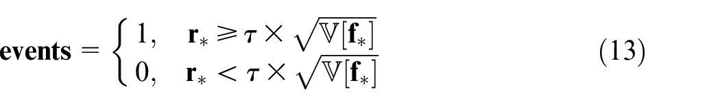
where
Interpreting the graphs: Demo data
This section presents a short tutorial on interpreting the graphical tools produced by the methods described above. For the purpose of this paper, analysis is restricted to five outputs from the artefact probing procedure, though the developed framework can process all items shown in Figure 5. Specifically, these are:
Axis checks
Probe checks
A synthetic dataset was generated for the purposes of this demonstration, and to select appropriate kernels and hyperparameter optimisation ranges for the GP methods. Data points were simulated over an eighteen-month period, representing the normal operation of a typical machining centre. Certain notable characteristics were introduced into the dataset to illustrate the graphical effects that the proposed methods should have. These are:
A significant event, or hard fault, occurs in the Primary-axis trend, on 2017-12-28.
A significant event, or hard fault, occurs in the Secondary-axis (+ve) and Secondary-axis (–ve) trends, on 2018-05-02.
The tolerance is changed for Primary-axis, on 2018-03-14; tolerance is changed for Secondary-axis (+ve) and Secondary-axis (–ve), on 2018-05-07.
There are no recorded out-of-tolerance measurements in the Overall probe performance and Probe pre-travel data.
Figures 6 shows the learnable tolerance threshold method, as applied to the demonstration dataset. On the format; measurements are plotted in a single dimension along the X-axis, with separate symbols for in-tolerance and out-out-tolerance class labels. Actual tolerance threshold changes are tagged at their corresponding values, with the date at which each was changed referenced to the right. The data-driven tolerance threshold is represented by the red-green colourmap, with the data-driven tolerance threshold at the decision boundary and two class separations on either side.
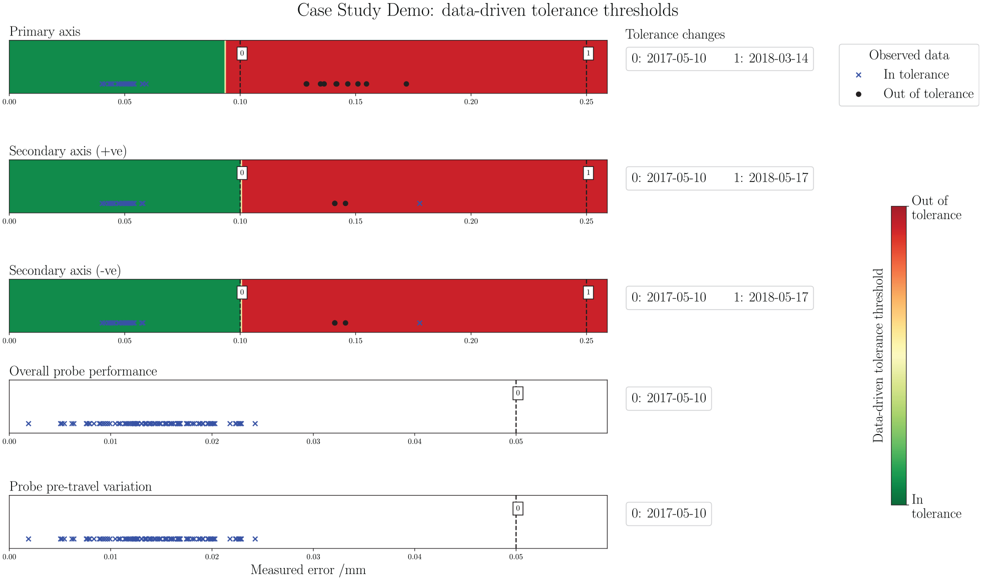
Demo data: data-driven tolerance thresholds. From top to bottom: Primary-axis, Secondary-axis (+ve), Secondary-axis (–ve), Overall probe performance, and Probe pre-travel. Tolerance change occurrences in the data acquisition period are noted alongside each graphic.
There are certain indicators in this data presentation which can provide an instant appraisal for understanding how the machine has performed with respect to the tolerance thresholds, and how the thresholds themselves have been managed. Following the initial setting on 2017-05-10, the tolerance changes on 2018-03-14 and 2018-05-07 are immediately clear, with flags indicating their respective increases from 0.1 to 0.25 mm. The data-driven thresholds for all three axis checks closely match the threshold set by the engineer initially; suggesting that, based on past-usage, the later threshold changes may be unwarranted. For the two Secondary-axis checks, it is noteworthy that one of the in-tolerance observed points lies in the out-of-tolerance zone designated by the data-driven threshold. Due to the threshold increase on 2018-05-17, this measurement – which is the highest value seen in the dataset – concludes that the machine is capable and fit for production. This change may be completely logical – the result of a new part in production and corresponding new tolerance requirements, for example; it could also represent an unwarranted change by the operator, in order to pass a test which would otherwise fail. The latter could have serious consequences for finished part quality. In either case, the learnable tolerance threshold and the graphical display shown in Figure 6 gives instant access to this information, for either the onsite ME or visiting specialist to interrogate. For the probe checks, all measurements were recorded as in-tolerance, and subsequently a data-driven threshold was not constructed. This information, along with the ME-set threshold and distribution of the data, is, again, quickly accessible from the display.
Figure 7 shows the trending GP method with intelligent event detection, as applied to the demonstration dataset. Each subplot presents the time-series information along the X-axis and measurement recorded by the artefact probing procedure on the Y-axis. Observed measurements are shown in a scatter plot, with separation for the data used to train and test the trending GP. The mean function,
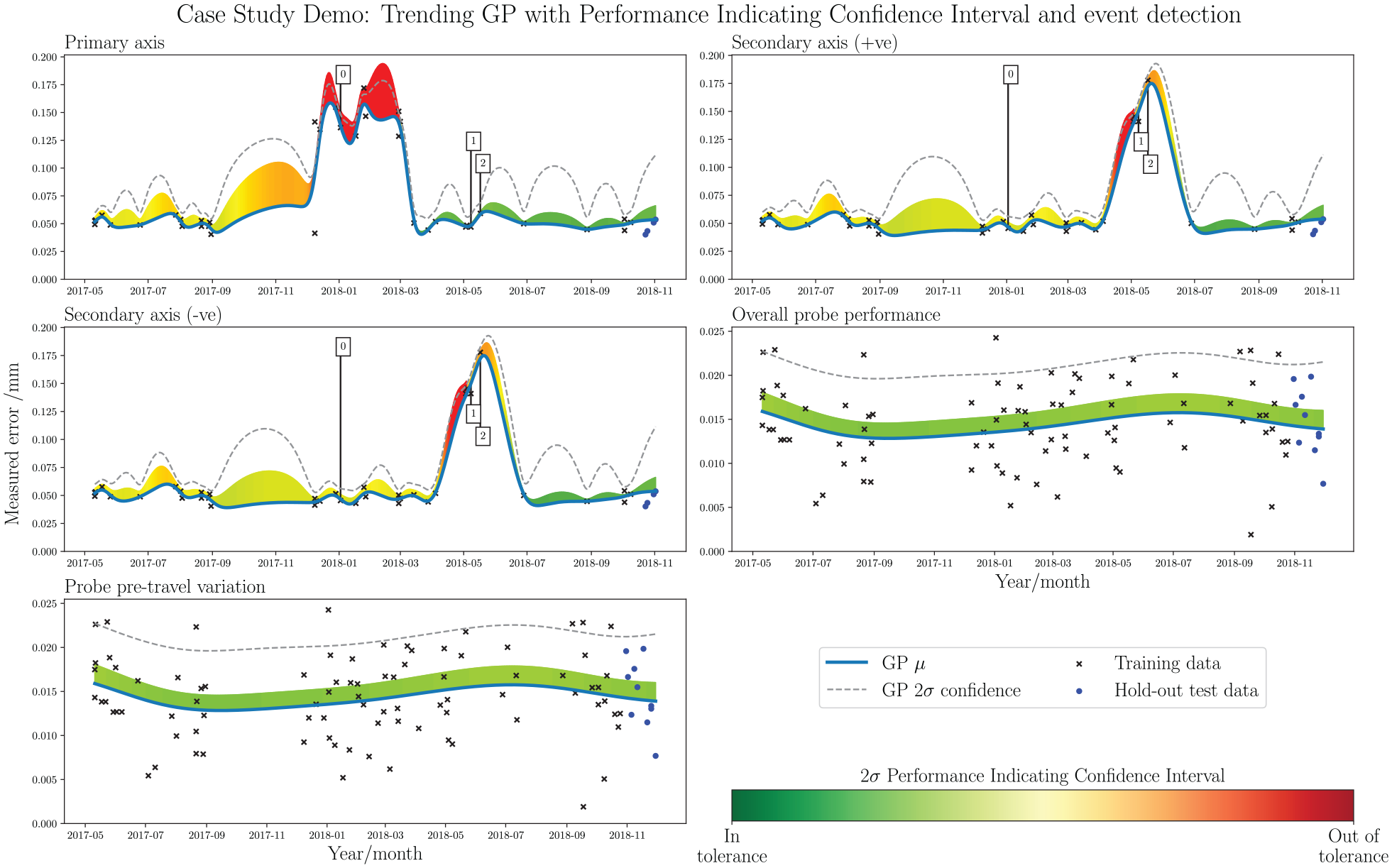
Demo data: trending GP with PICI and event detection. Significant events occur at 2017-12-28 and 2018-05-02. Each subplot shows a different data stream, derived from the extrapolation of the elements in the benchmark summary of Figure 5. From top left: Primary-axis, Secondary-axis (+ve), Secondary-axis (–ve), Overall probe performance, and Probe pre-travel.
The graphical representation shown in Figure 7 provides fast access to legacy data, displayed over the collection period. The two significant events, on 2017-12-28 for the Primary-axis and 2018-05-02 for the Secondary-axis, are clearly visible by spikes in the GP mean function. In both cases, the event detector accurately flags the problem regions. PICI colourmapping shows that there is an exceedance of the tolerance threshold in both of these regions. The most extreme measurement following the Secondary-axis event on 2018-05-02 shows a tolerance change, as the PICI colour drops from red to yellow, even though the measured error increases. The representation also shows the consistency of data collection, with taller
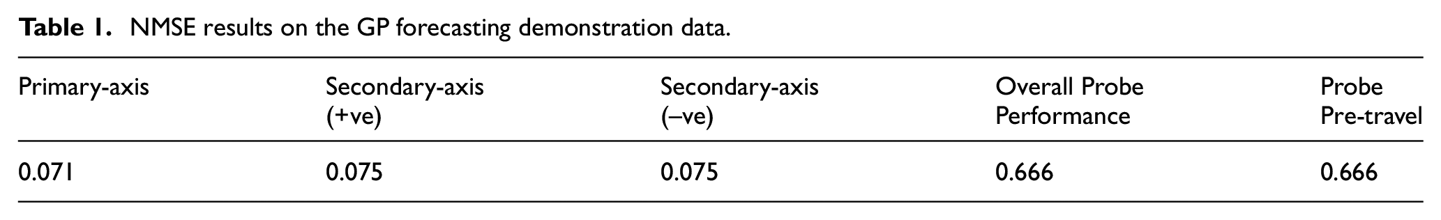
A test set was held out prior to model training to asses the practicality of predicting future trends with this method. The Normalised Mean Squared Error (NMSE) is applied to evaluate the model performance in predicting near-future events. NMSE values below 1.000 signify the existence of correlation between the test set observations and model prediction, NMSE values above 1.000 suggest poorer performance than simply applying the mean of the data as the predictor. 29 The results are presented in Table 1. For the demonstration dataset, the results are reasonable; particularly in the axis checks, where they are very low, indicating a notable correlation between observations and model predictions. The probe checks are less impressive, but still better than simple application of the mean value. However, predicting a future trend in this way relies on the assumption that proceeding data points will follow a similar pattern; in other words, it is only reliable for predicting soft fault trends. However, hard faults can and do occur throughout the life-cycle of a typical machining centre, which ultimately is the motivation for intelligent event detection highlighted in this paper. For this reason, such an approach to trend analysis will never be appropriate for predicting future states, and can not be implemented for a monitoring system which relies solely on artefact probing data. Given the scope of this paper, however, this does not affect the efficacy of the proposed methods, as the core focus is one of legacy data visualisation for fast appraisal of machine usage.
NMSE results on the GP forecasting demonstration data.
Kernel selection
The kernel (covariance function) chosen for a GP model can significantly impact the resulting form of the predictor. The Radial Basis Function (RBF), otherwise known as the Squared-Exponential kernel, is a popular kernel selection which is infinitely differentiable and thus very smooth. It is parameterised by a non-negative length-scale parameter,
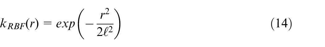
where
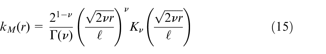
where
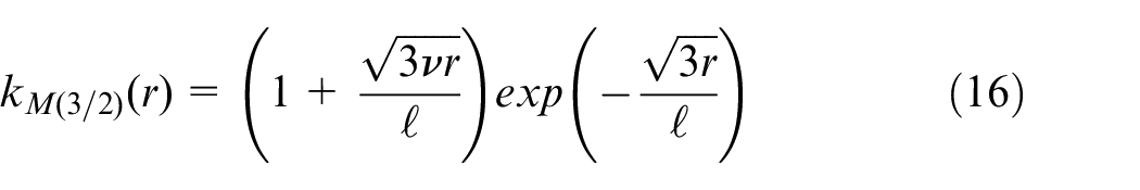
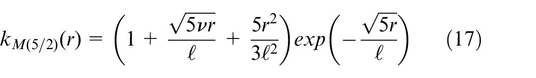
Setting
Finally, the Rational Quadratic (RQ) kernel represents a scale mixture of RBF kernels with different length-scales, given by,
where
Comparing five different kernels for the trending GP, on the Primary-axis procedure. Kernels from top left: Rational Quadratic, Radial Basis Function, Matérn 5/2, Matérn 3/2 and Matérn 1/2.
Considering the comparison in Figure 8, the RQ kernel presents itself as the most appropriate option for modelling the time-series trend. There is minimal inflection between observations, and the mean function fits smoothly when it passes through more densely-populated regions. The
Figure 9 presents the same kernel comparison, but as applied to the GP event detector method. Each subplot shows the residual values for the different kernel selections by a blue, solid line, with a
Comparing five different kernels a GP event detector, with simulated events at 2017-12-28 and 2018-05-02. Kernels from top left: Rational Quadratic, Radial Basis Function, Matérn 5/2, Matérn 3/2 and Matérn 1/2. The 3
Observing the subplots in Figure 8, it appears that the GP residuals generally peak as intended when events occur for all kernel options. The weakest seems to be the RBF kernel, which activates less accurately for event 1 and misfires at the end of the acquisition period. RQ, and the three Matérn kernels, all produce similar trends. Considering the threshold values obtained through the GP variances, the RQ kernel is the only option to produce a reasonably smooth threshold, whereas the RBF and Matérn options result in erratic thresholds. A smoother, more predicable decision boundary is preferable for this application, as large, unexpected jumps may result in false positive event detection, such as that which occurs in the RBF/Matérn systems around 2018-09. For these reasons, the RQ kernel was selected as most appropriate for the event detector. The setting of the novelty threshold could be varied based on requirements, and the experience of the ME responsible. However, for this assessment, a conservative
Case studies
This section now presents three case studies on engineering datasets, acquired directly from anonymised industrial partners. The processing and display of results for each method are identical to those which are introduced in the previous section, Interpreting the graphs: Demo data.
Case study 1
Figure 10 presents the threshold checking tool for case study 1. It is clear that the threshold has been changed numerous times throughout the acquisition period, which may indicate a mixture of parts for production with varying tolerance requirements. In the axis checks, however, many of the tests have returned out-of-tolerance class labels. This suggests that the machine has been consistently not conforming to the tolerance requirements, reflecting a poor monitoring strategy which may ultimately lead to issues with finished part quality. The threshold-checking presentation makes this inference immediate and easily accessible.
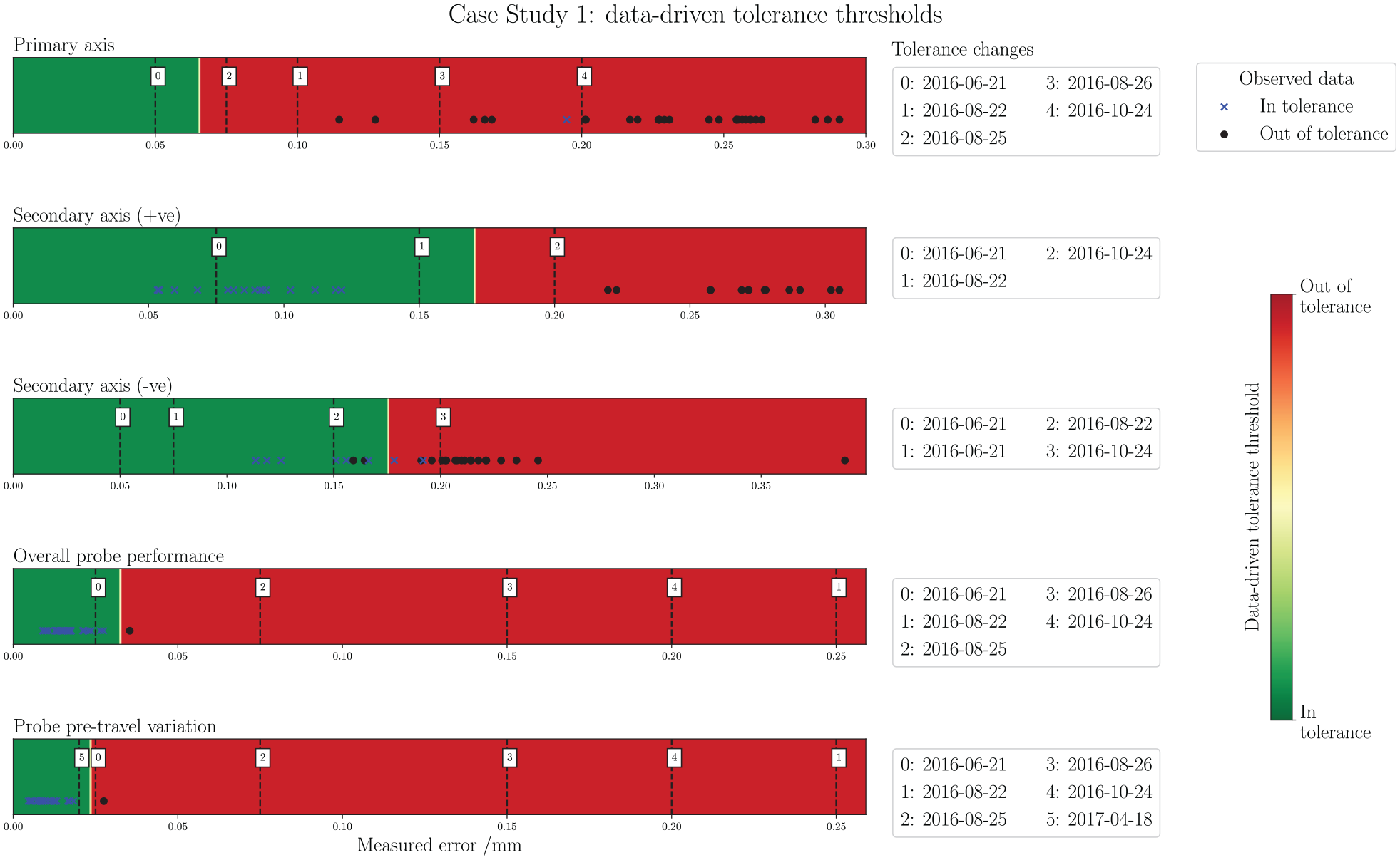
Case study 1: data-driven tolerance thresholds. From top to bottom: Primary-axis, Secondary-axis (+ve), Secondary-axis(–ve), Overall probe performance, and Probe pre-travel. Tolerance change occurrences in the data acquisition period are noted alongside each graphic.
Table 2 presents the F1 scores for the data-driven threshold classifiers. The data is linearly separable in three of the five cases, returning F1 scores of 100% in the test set. In the other two there is some crossover, so the soft margin parameter permits some misclassification, however the F1 scores are still very good, at 99% for the Primary-axis and 89% for the Secondary-axis (–ve). In all but Primary-axis, a tolerance threshold is optimised which logically separates the observations. The threshold for the probe checks very closely resembles the final ME setting for Probe pre-travel, and gives a similar but slightly more conservative setting for Secondary-axis (+ve) and (–ve). In the Primary-axis, there is only one in-tolerance observation available to construct the threshold which is mixed deep within the cluster of the other class. As a result, the calculation is biased towards the simulated ideal data points, and the threshold is constructed at a very conservative (low) value. Although this isn’t likely to be an appropriate tolerance setting, it is a logical conclusion for the algorithm based on the historical data, and is a further red flag pointing towards mis-management of the tolerancing in this case study.
F1 scores on a 10% hold-out test set, for the 1D-SVM data-driven tolerance threshold.
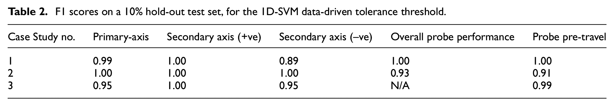
Figure 11 shows the output of the trend analysis tool as applied to case study 1. The PICI integration paints an immediate picture of the error states with respect to tolerance thresholds throughout the acquisition period, particularly when viewed alongside Figure 10. In Primary-axis, it is clear that the machine has been running consistently out-of-tolerance. Closer inspection of the
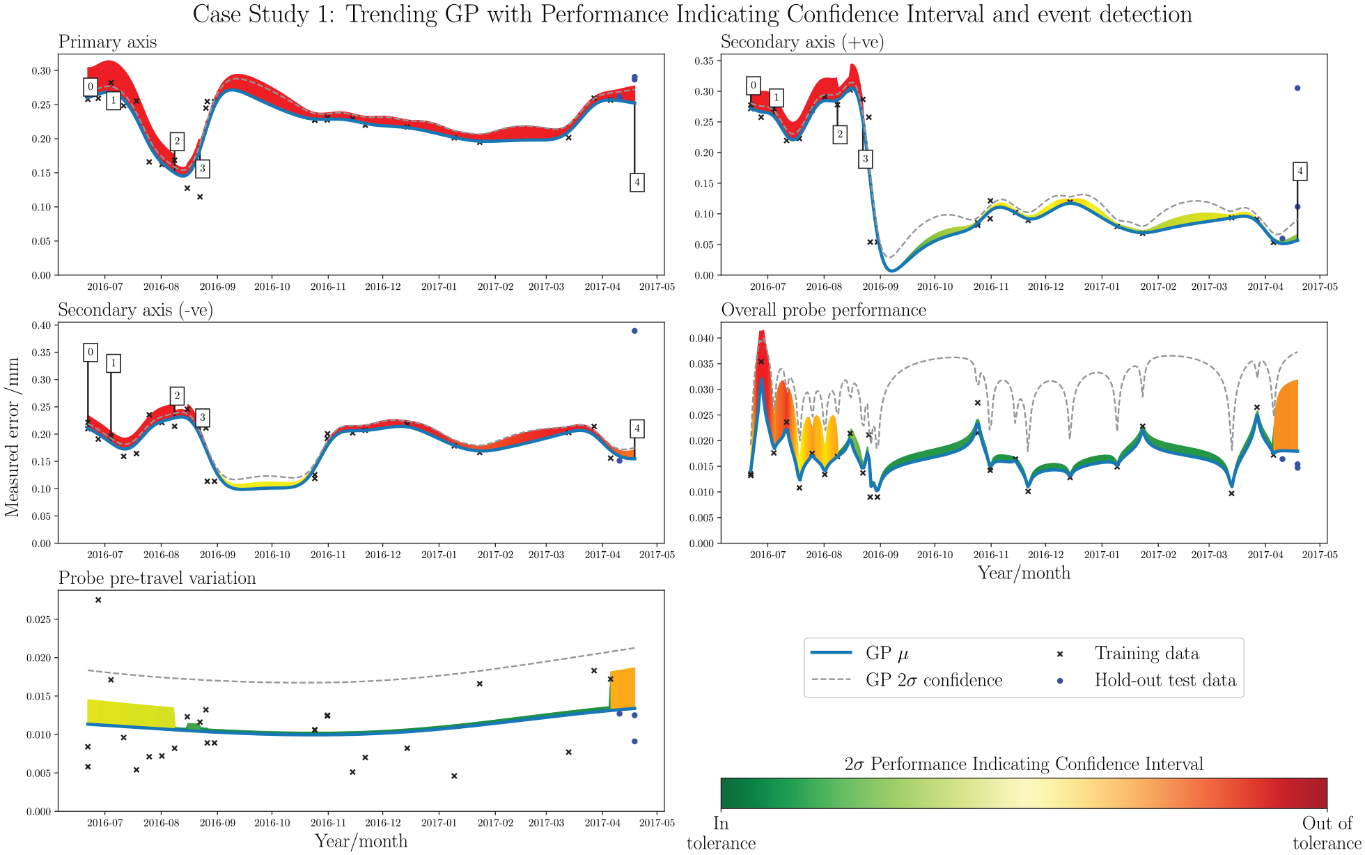
Case study 1: trending GP with PICI and event detection. Each subplot shows a different data stream, derived from the extrapolation of the elements in the benchmark summary of Figure 5. From top left: Primary-axis, Secondary-axis (+ve), Secondary-axis (–ve), Overall probe performance, and Probe pre-travel.
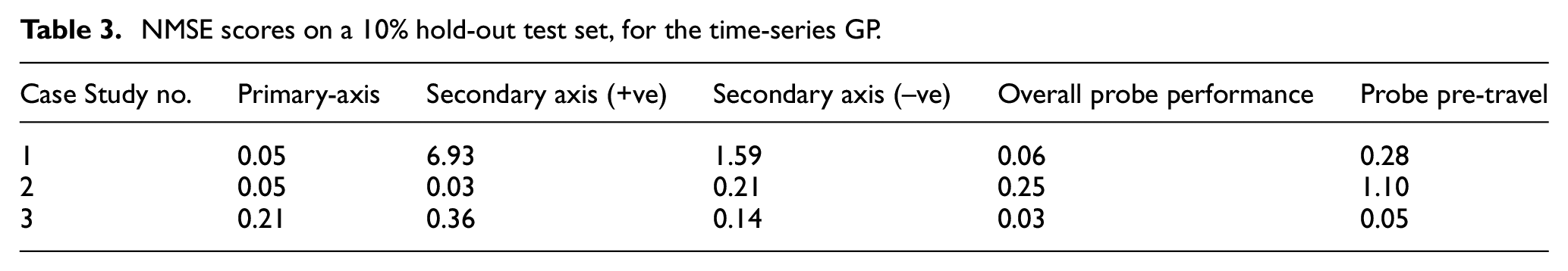
NMSE scores on a 10% hold-out test set, for the time-series GP.
Case study 2
Figure 12 presents the threshold checker for case study 2. All three axis checks are linearly separable between the two classes, which is immediately clear in the Figure and also by the F1 scores in Table 2. This separation indicates a methodical approach to setting the tolerance thresholds, and that the machine is likely to be under relatively constant tolerance conditions throughout the operating period. In all cases, a set of sensible tolerance thresholds were learned which closely reflect most of the final values settled on by the ME. The exception to this is in Secondary-axis (+ve), which sees a peculiar increase to
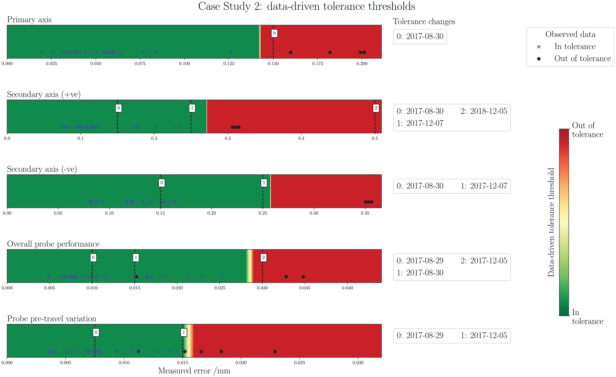
Case study 2: data-driven tolerance thresholds. From top to bottom: Primary-axis, Secondary-axis (+ve), Secondary-axis (–ve), Overall probe performance, and Probe pre-travel. Tolerance change occurrences in the data acquisition period are noted alongside each graphic.
Figure 13 presents the trending GP tool for case study 2. The probe checks provide a good example of the PICI visualisation, giving a clear indication of the historical performance and out-of-tolerance instances around 2018-08/09. NMSE results indicate decent soft trend predictive performance, with only Probe pre-travel producing a high value above 1.000. It is evident that the accuracy of the Primary-axis deteriorates towards the end of the acquisition period, which accounts for the out-of-tolerance points observed in Figure 12. There is clearly a hard fault which occurs in 2017-12, causing a spike in the trend; however, as corrective action was immediately applied, the full magnitude of the error is not reflected. Although the full extent of the tolerance exceedance is not visualised in the trend, this is actually a better representation of the machine’s general history, as the hard fault occurs for an insignificant duration in the overall chronology. The graphical presentation does, however, provide a visual prompt of this region as an area of interest for the interrogating ME or visiting specialist. The event detector - trained on the stable period of normal operating condition between 2018-02 and 2018-10 - exactly identifies a hard fault event on 2017-12-07 in the Secondary-axis, and also identifies a soft fault event in both Primary-axis and Secondary-axis (+ve) later in the time series, identifying a degradation from 2018-10-15. It must be noted that the method relies on consistent data collection across all of the input variables; the final four collections after 2018-10-15 omitted Secondary-axis (–ve), as such it was necessary to omit these points when computing the event detector. As the last data point collected for Secondary-axis (–ve) did indicate the presence of a fault, the system was able to pick it up. However, it is a noteworthy restriction of the method, and a commercially-deployed system should consider robustness to inconsistencies in data pre-processing.
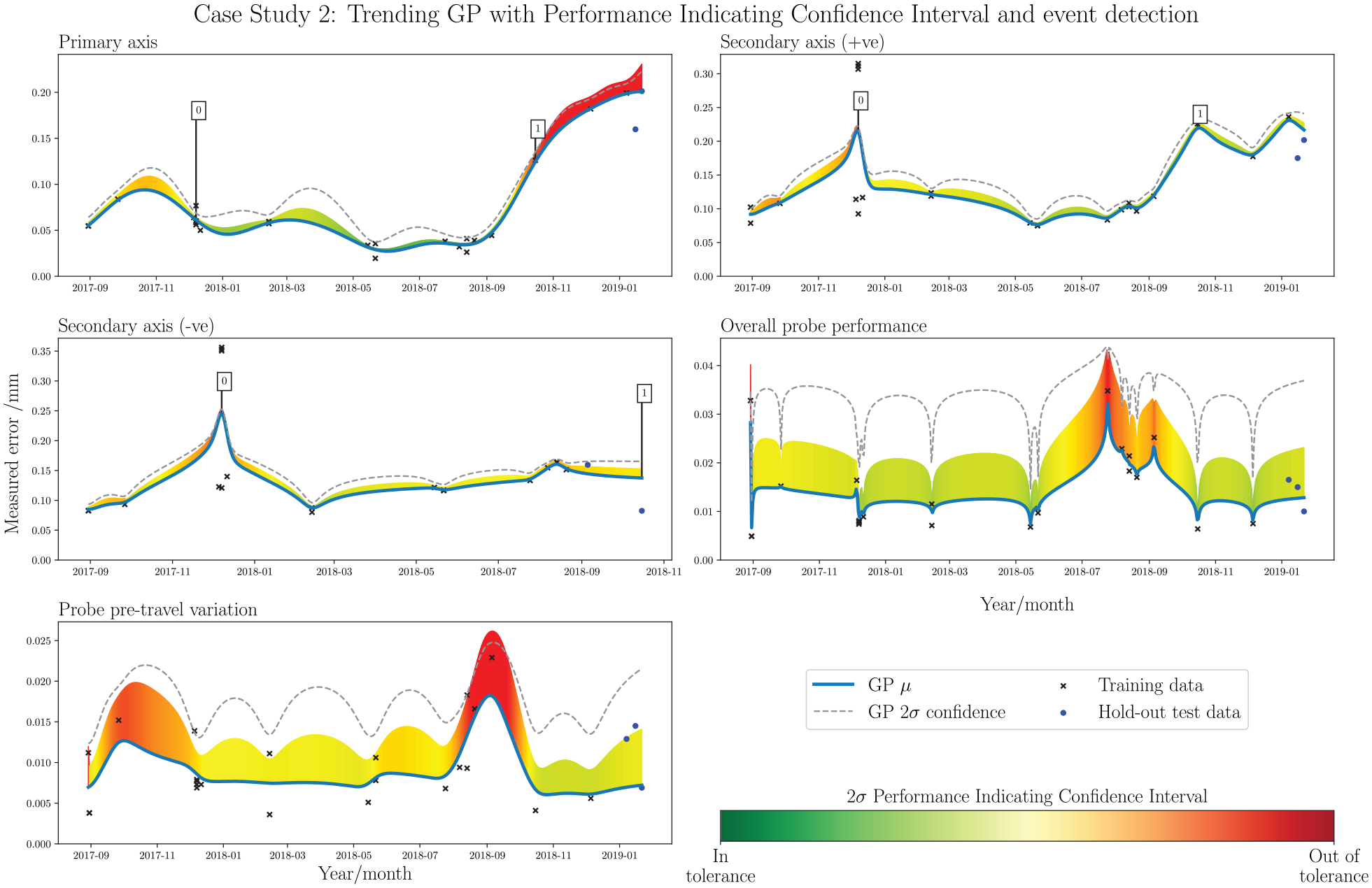
Case study 2: trending GP with PICI and event detection. Each subplot shows a different data stream, derived from the extrapolation of the elements in the benchmark summary of Figure 5. From top left: Primary-axis, Secondary-axis (+ve), Secondary-axis (–ve), Overall probe performance, and Probe pre-travel.
Case study 3
Figure 14 presents the threshold checking method as applied to case study 3. Immediately apparent is the lack of a data-driven threshold for Overall probe performance and failed construction of a data-driven threshold in Probe pre-travel. In the case of Probe performance, this indicates that all measurements were considered by the ME as in-tolerance. This is generally good news; however, it is also clear that many of the points are situated quite closely to the first tolerance change (2017-05-11); at
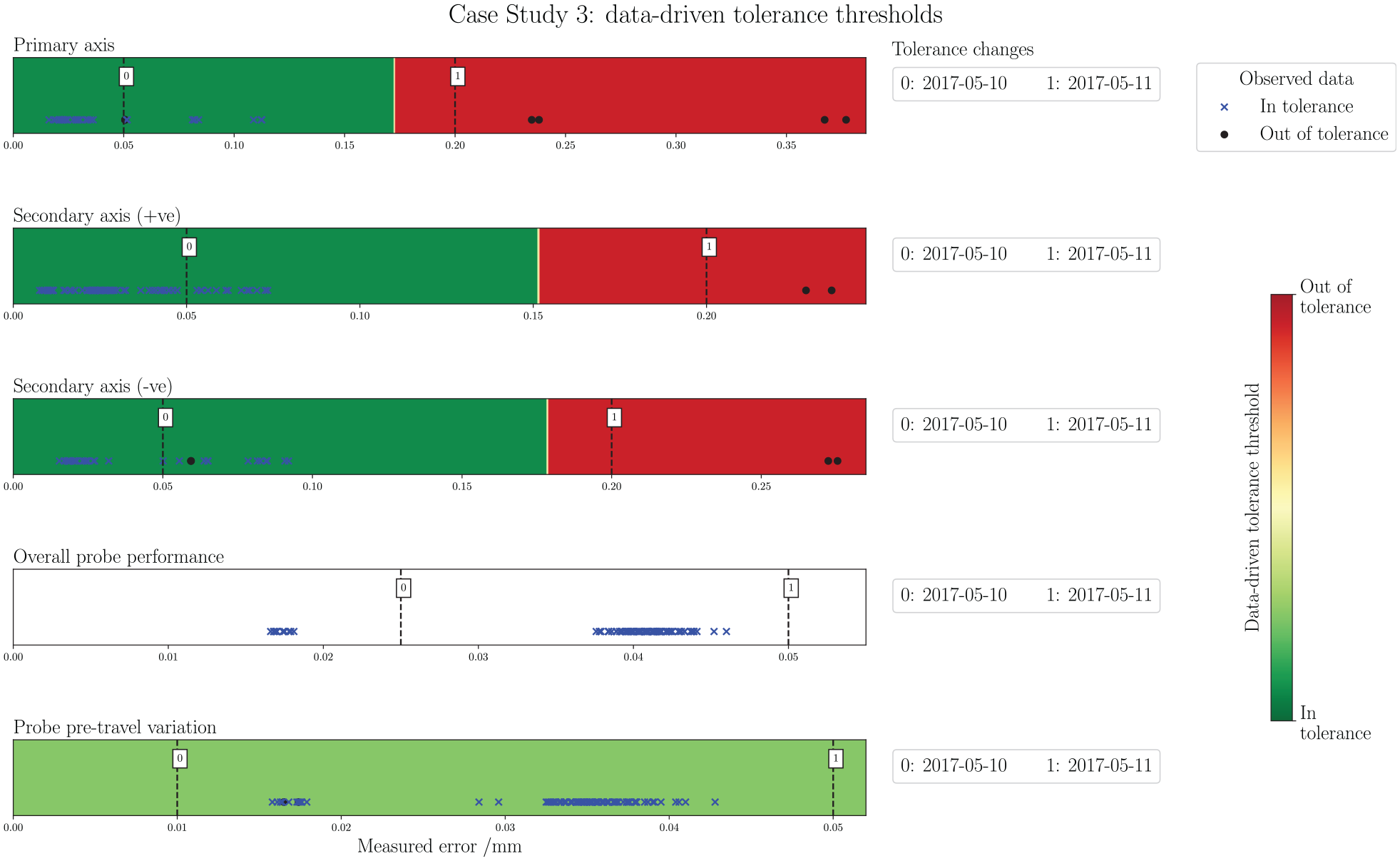
Case study 3: data-driven tolerance thresholds. From top to bottom: Primary-axis, Secondary-axis (+ve), Secondary-axis (–ve), Overall probe performance, and Probe pre-travel. Tolerance change occurrences in the data acquisition period are noted alongside each graphic.
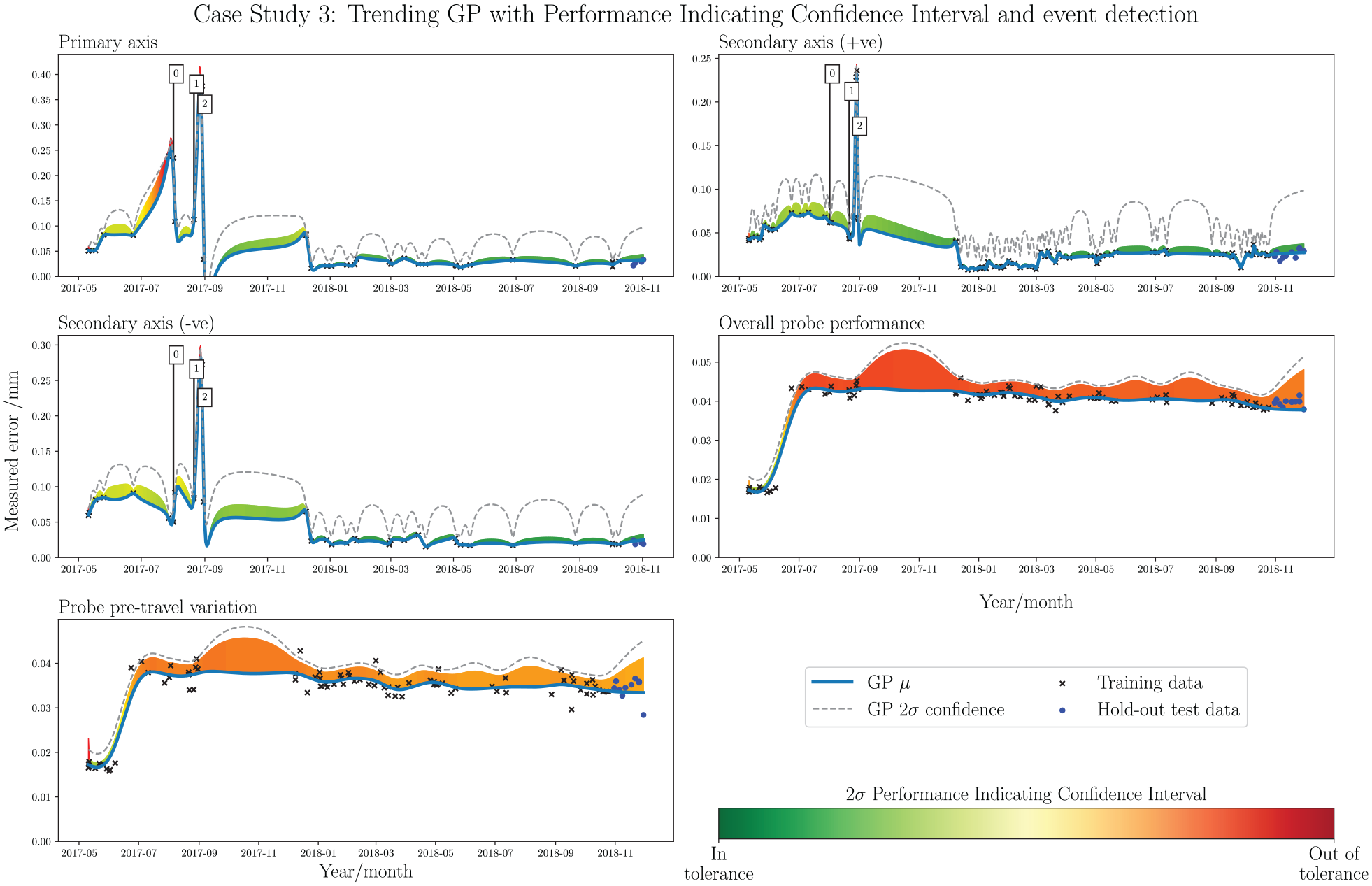
Case study 3: time series trend analysis with PICI and event detection. Each subplot shows a different data stream, derived from the extrapolation of the elements in the benchmark summary of Figure 5. From top left: Primary-axis, Secondary-axis (+ve), Secondary-axis (–ve), Overall probe performance, and Probe pre-travel.
The trending GPs in Figure 15 indicate the presence of hard faults around 2017-08-01 and 2017-08-28, which are also clearly visible as the out-of-tolerance points in Figure 14. The event detector, trained on the stable period between 2017-12 and 2018-05, accurately picks out the events, with a second trigger also occurring close to the second. The probe checks with PICI illustrate both the general trend and measurements with respect to tolerance threshold nicely. It is instantly clear that the recorded measurements were close to the specified tolerance throughout most of the acquisition period. The NMSE results in Table 3 indicate favourable performance for predicting future observations with these trends, due to the highly stable behaviour that is observed from 2018-01 onwards. One point to note is that the trend in the Primary-axis does dip below zero for a short time, following correction of the hard fault detected on 2017-08-28. Although the selected kernel and hyperparameter settings drastically reduce the likelihood of this happening, the occurrence in this case study shows that it has not been entirely eradicated. In a full deployment system, it may be worthwhile to include an extra step following the trending GP construction, in which any below-zero regions are replaced by more logical above-zero values; for example, by a linear interpolation between the two neighbouring datapoints.
Case studies: Comparison
The standardised analysis and visualisation techniques presented in the previous section give rise to the possibility machine usage comparisons between the three case studies. Comparing the tolerance threshold changes in Figures 10, 12 and 14, it is evident that the three machines have been managed in very different ways. In case study 1, there are are numerous changes to the tolerance threshold throughout the acquisition period, and it is also clear that many of the measurements obtained fell into the out-of-tolerance class. This is a particular contrast to case study 3, which indicates no change to the tolerance after the initial setting period and a majority of measurements firmly in the in-tolerance class. This suggests a more consistent management approach in case study 3, with much better adherence to the tolerance thresholds that were initially set by the onsite ME.
Comparing the trends in Figures 11, 13 and 15 reveals similar characteristics. It is observed that the PICIs for the axis checks in case study 1 regularly exceed the tolerance thresholds throughout the acquisition period; this a direct contrast to the axis checks in case study 3, where there is clearly a short period involving a hard fault near the beginning of the period, followed by strict conformance to the tolerances thereafter. Case study 2 generally indicates conformance to the tolerances in the axis checks, with a similar hard fault visible early in the acquisition period. However, there is evidence of a soft fault developing towards the end of the period in case study 2 axis checks, which is a notably different characteristic to the other case studies and easily recognisable in the trend visualisation.
An interesting observation is found in comparing the probe checks, where there is significantly lower variance in the trends for case study 3 as compared with case studies 1 and 2; this likely indicates that the probing procedure is more repeatable across different instances of the procedure conducted at different times. The proprietary software currently contains a check to assess the repeatability of the probe at the time of the test, however interpretation of the trending GPs proposed in this paper allow straightforward extension of this for the purpose of longer-term performance monitoring.
Discussion
Historical machine indicators - such as the prevalence of hard or soft faults, long-term probe repeatability of tolerance management practices – can be very useful for building up a picture of general machine usage, and are available through the appropriate processing of a relatively limited data source obtained from historical artefact probing data. Moreover, the unique compositions of indicators observed in different machine tools support the notion of signature comparison; just as the benchmark reports can be used to compare differing signatures of machine tools within a population, so too can the methods proposed in this paper be used for comparing signatures that represent machine tool usage.
Similar to the signature, any given machine also has a normal operating condition, which may differ in a small or large way to another machine considered its counterpart. The objective with producing a data-driven tolerance threshold, as opposed to relying solely on the maintenance engineer determination, is that it is possible to set the most appropriate tolerance which represents the normal operating condition of the unique machining centre. Learning tolerance thresholds in this way provides the ME which an additional empirical comparator for assessing the performance of a population of machines, based on historical data collected throughout their respective usages.
A key contribution of this paper is in the organisation and presentation of the historical data, significantly reducing the difficulty for an onsite ME or visiting specialist engineer to gain a fast appraisal of a given machine tool’s usage signature. The display methodologies were produced with consideration to Tufte’s design principles, which, although somewhat subjective, should support effective communication of the data with a reasoned application of visual aesthetics. The Performance Indicating Confidence Interval is an example of this, enhancing the trending Gaussian Process into a multifunctional element which communicates both the absolute error trend, and provides the context of performance by integrating the variable tolerance thresholds throughout the acquisition period.
In a full deployment situation, the benefit to the user would be significantly increased through the use of an interactive dashboard-style interface. Displaying the data-driven tolerance and trending Gaussian Process tools side-by-side and having a linked hover-over function – such that, when an observation is hovered over on one method, it is highlighted in the other – would be a useful feature, providing a richer user experience and making the graphs easier to interpret. The hover-over function should also provide quick access to the relevant detailed reports, making in-depth analysis in areas of interest easier to conduct.
It is noted that the smoothness of the predictive mean function - attributed to kernel and kernel hyperparameter selection – affects the resultant form of the trending Gaussian Process. With a smoother mean function, quickly-corrected hard faults are not as readily represented in the trend; this is more suitable for visualising the general historical performance, and the addition of the event detection method should help bring attention to these quick corrections of hard faults, but in a more appropriate manner. Normalised Mean Squared Error results on a hold-out test set at the end of the acquisition period evaluated the potential for using the trending Gaussian Process as a forecasting method. It was initially expected that this would not be an effective application for forecasting, due to the likelihood of hard faults interrupting any predicable, soft trends. As the core objectives with the trending Gaussian Process are trend visualisation and enrichment of historical data, this drawback does not affect the contribution of this paper. In order to reliably forecast future performance in a system like this, peripheral data streams could be utilised to identify the occurrence of hard faults, or progression of soft faults, adjusting the prediction accordingly. This functionality is out of the scope of this paper, but would be interesting future work.
The automated event detection system was shown to be effective at identifying target events, in both the simulation dataset and the three real-world case studies. In a fully deployed system, consideration must be given to defining a suitable subset for training, as the initial data acquisition period for real-world systems is not guaranteed to be free from events and representative of the normal operating condition. The datasets generated for this application are not likely to be large, so it would be appropriate to allow an experienced user the ability to retrospectively reset the training period, should the requirement arise. The event detector flags in a fully-deployed system would, again, benefit from an interactive interface, with the option to manually input diagnostic notes. Automating this diagnostic element to populate the notes without user input would be valuable further research.
Concluding remarks
The methods set out in this paper develop the information acquired from a common machine capability checking system, into a performance monitoring system for the benefit of the onsite maintenance- and visiting specialist-engineers. Performance indicators such as the incidence of hard and soft faults, management of tolerance thresholds and repeatability of measurements are identified within the datasets, and brought to the attention of the engineer through automated analysis and insightful data visualisation. The methods process only the summary statistics obtained via a calibrated artefact probing procedure; to develop the work further, this could be expanded to consider all of the raw artefact probing data, as well as information obtained from external sources as part of a wider manufacturing execution system. This would allow a much richer level of inference to be attained, including more extensive automated elements to further enhance the benefit to the user.
Footnotes
Acknowledgements
The authors would like to gratefully acknowledge metrology software products ltd. and the Engineering and Physical Sciences Research Council (EPSRC) grant EP/I01800X/1 for supporting this research. KW would like to additionally acknowledge support from an EPSRC Established Career Fellowship EP/R003645/1.
Declaration of conflicting interests
The author(s) declared the following potential conflicts of interest with respect to the research, authorship, and/or publication of this article: The research project was conducted in collaboration with industrial partner metrology software products ltd. (msp). In accordance with this partnership, the primary application of the work is in developing an msp procedure for performance monitoring; however, the methods presented are generic, and can be applied to any other techniques that utilise artefact probing for similar purposes.
Funding
The author(s) disclosed receipt of the following financial support for the research, authorship, and/or publication of this article: This research was supported by EPSRC grants EP/I01800X/1 and EP/R003645/1, and metrology software products ltd.