
Abstract
5-Degree-of-freedom parallel kinematic machine tools are always attractive in manufacturing industry due to the ability of five-axis machining with high stiffness/mass ratio and flexibility. In this article, error modeling and sensitivity analysis of a novel 5-degree-of-freedom parallel kinematic machine tool are discussed for its accuracy issues. An error modeling method based on screw theory is applied to each limb, and then the error model of the parallel kinematic machine tool is established and the error mapping Jacobian matrix of 53 geometric errors is derived. Considering that geometric errors exert both impacts on value and direction of the end-effector’s pose error, a set of sensitivity indices and an easy routine for sensitivity analysis are proposed according to the error mapping Jacobian matrix. On this basis, 10 vital errors and 10 trivial errors are identified over the prescribed workspace. To validate the effects of sensitivity analysis, several numerical simulations of accuracy design are conducted, and three-dimensional model assemblies with relevant geometric errors are established as well. The simulations exhibit maximal −0.10% and 0.34% improvements of the position and orientation errors, respectively, after modifying 10 trivial errors, while minimal 65.56% and 55.17% improvements of the position and orientation errors, respectively, after modifying 10 vital errors. Besides the assembly reveals an output pose error of (0.0134 mm, 0.0020 rad) with only trivial errors, while (2.0338 mm, 0.0048 rad) with only vital errors. In consequence, both results of simulations and assemblies validate the correctness of the sensitivity analysis. Moreover, this procedure can be extended to any other parallel kinematic mechanisms easily.
Introduction
Nowadays, five-axis machine tools play more and more important roles in the manufacturing industry for their convenience in accomplishing five-axis machining without repeatedly clamping workpieces and setting tools. Meanwhile, because of the multi-closed-loop architecture, parallel kinematic mechanisms (PKMs) are regarded to have theoretical advantages over serial kinematic mechanisms (SKMs) of higher stiffness/mass ratio and flexibility. 1 Therefore, parallel kinematic machine tools (PKMTs) are potential to realize five-axis machining of complex curving workpieces in a more compact and efficient way than the traditional serial kinematic machine tools (SKMTs). However, few of existing 5-DoF fully PKMs2–5 are suited for and have been developed into PKMTs. Xie et al.6,7 designed a novel 5-DoF PKM in 2014 and then analyzed the issues of mobility, singularity, kinematics, and dimensional synthesis. It has only three limbs to realize 5-DoF motion with 90° orientational capability, where two of them are planar substructures each composed of two links. This architecture guarantees both flexibility and the ability of five-axis machining, so it is promising for industrial application as a PKMT, and our paper will focus on this PKM.
Like all the other PKMTs, accuracy problem is always one of the main concerns. Although intelligent methods 8 are rapidly developing, accuracy design 9 and kinematic calibration5,10 are still the less costly tools with wider applicability. In general, accuracy design is by allocating tolerances for geometric error parameters to restrict the range of output pose errors before PKMTs are built, while kinematic calibration is by measuring output pose errors to identify real geometric errors after PKMTs are assembled. Therefore, it is fundamental to grasp the relationships between output pose errors and geometric errors and is significant to estimate the effects of geometric errors on output pose errors. In fact, error modeling and sensitivity analysis are the prerequisites for accuracy problem of PKMTs.
There are several mathematical methods to establish the error model of PKMs. Closed-loop vector chain (CVC) method is a widely used approach for its concise and straightforward expression.9–12 However, Wang et al. 13 pointed out that there exist three different formats to express a single error vector and thus it is hard to find a unified and optimal error model with CVC method. Denavit–Hartenberg (D-H) homogeneous transformation (HT) method is another conventional approach for error modeling.14–17 This method is somewhat attractive for its four-parameter representation of adjacent local reference frames located at each joint, which means D-H parameters are one of the minimal parameter sets with distinct physical meaning. 15 However, if two consecutive joint axes are collinear, this method will develop error models neither complete nor parametrically continuous. 16 Although Zhuang et al.16,17 proposed a modified version of D-H modeling convention with completeness and parametric continuity properties, complex operations restricted its promotion.
Screw theory is another powerful tool to establish error models, not only due to its benefits of expressing revolute and prismatic joint motions in a complete and uniform representation with clear physical meaning,18,19 but also because its modern geometric interpretation is the basis of the product of exponentials (POE) with the algebraic property of continuous differentiability.20–23 However, the POE method is seldom applied to PKMs, 23 since it cannot formulate the constraint properties of low-mobility PKMs. 24 To extend the application of screw theory, Liu et al. 25 proposed a general error modeling method for PKMs in 2011 and applied it to three classical low-mobility PKMs, Sprint Z3 spindle head, Tricept, and Delta. Although this approach has covered most of the typical limbs and structures,5,25,26 PKMs with substructures are barely included, let alone the novel architecture with special limbs studied in this article, which means it needs to be further studied.
When the error model is established, it means that the corresponding error mapping Jacobian matrix (EMJM) is derived, which essentially reflects the linear impacts of each error parameter on the end-effector’s pose errors. On this basis, sensitivity analysis can be implemented to find out which error parameters are vital error sources and which are trivial. Interval method,12,27 probabilistic method,11,28 and linearization method29,30 are three commonly used approaches. However, all of the sensitivity indices (SIs) resulting from these methods are directly (linearization and probabilistic method) or indirectly (interval method) in accordance to the two-norm of the column vectors of EMJM, which means only the values of errors are in consideration, while the directions of errors are neglected. Li et al. 31 proposed a new set of SIs and verified its feasibility on a five-axis SKMTs in 2016. These indices are derived from the inner product between the part of the pose error caused by each error parameter and the total of the pose error, so that the vector properties of errors can be embodied. In our opinion, this way of designing SIs is more effective due to its clearer physical interpretations than others and has good prospects when applied to PKMTs.
The remainder of this article is organized as follows. Section “Description of the PKMT” describes the architecture of the novel 5-DoF PKMT discussed in this article. Section “Error modeling” briefly introduces the error modeling method based on screw theory and then develops the error model of the PKMT accordingly. In section “Sensitivity analysis”, a set of SIs and an easy routine for sensitivity analysis are proposed, and the results are validated by several numerical simulations of accuracy design and three-dimensional (3D) model assemblies with geometric errors. Finally, some conclusions are given in the last section.
Description of the PKMT
The novel 5-DoF PKMT studied in this article is presented in Figure 1, and its inverse kinematics has been investigated in detail in Xie et al. 7
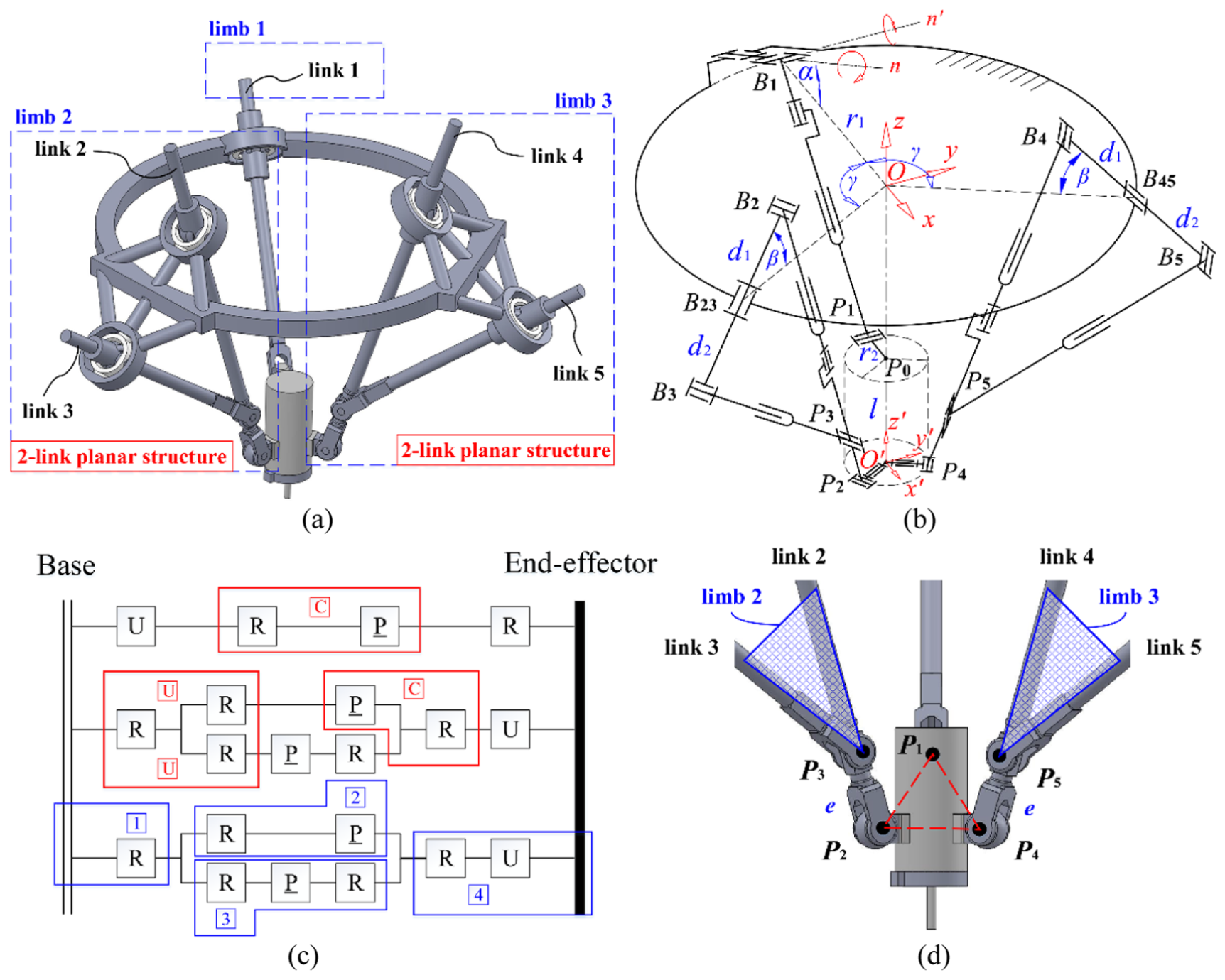
The novel 5-DoF PKMT: (a) 3D model, (b) kinematic scheme, (c) joint-and-loop graph, and (d) view of the end-effector.
As it can be seen from the 3D model in Figure 1(a) and the kinematic scheme in Figure 1(b), there are five links constituting three limbs to connect the base with the end-effector. Limb 1 (link 1) is a UR
Figure 1(c) is the joint-and-loop graph of the PKMT. It reveals some integrations of joints (in red) which are implicit in Figure 1(a) but explicit in Figure 1(b), and four divisions of joints in limb 2(3) (in blue) which will be explained in section “Error modeling for limb 2.”
Figure 1(d) shows the detailed view of the end-effector and presents the specialization of the two-link planar structure, which mostly comes from the distance e between point
Error modeling
As mentioned in section “Introduction”, an error modeling method based on screw theory would be applied to each limb of the PKMT under study. In general, this method consists of four steps, and the followings are a brief introduction:
Step 1: set up two global frames,
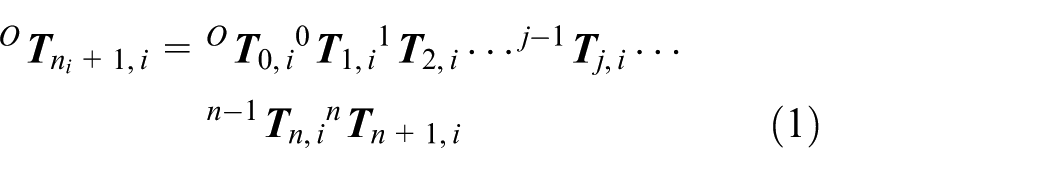
where
Step 2: bring in kinematic and geometric parameters of HTMs in equation (1) with small perturbations. Then the actual pose of the end-effector can be expressed by
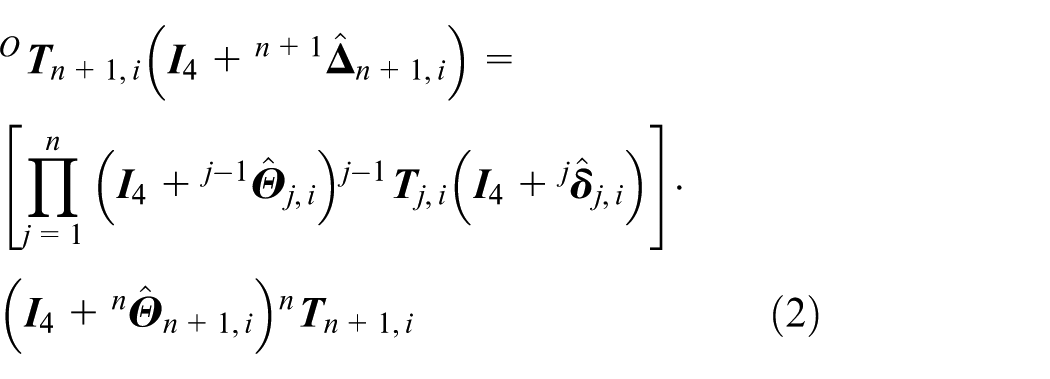
where
Step 3: expand equation (2), ignore higher-order terms with errors and equally express HTMs in the vector form by appropriate adjoint transformation. 32 Then the pose error of the end-effector in relation to first-order errors in the representation of Plücker coordinate can be obtained, and the concept of the screw can be brought in sequentially
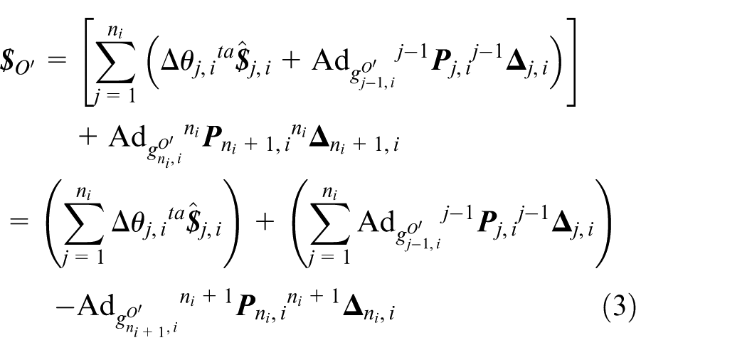
where
Step 4: remove the unknown kinematic errors of passive joints in equation (3) according to screw theory. 24 Then the error model of limb i can be established
where the subscript ka denotes the serial number of the actuated joint, and
The detailed expressions of symbols mentioned above can be checked in Appendix 1 and error modeling of most typical limbs for PKMs can be accomplished till here. However, if limbs are composed of substructures with any link not attached to the end-effector directly, there will exist some unknown kinematic errors of passive joints which cannot be removed by the active wrenches of the actuated joints, such as the limbs of two-link planar structures mentioned in section “Description of the PKMT”. This question will be solved in section “Error modeling for limb 2”.
Error modeling for limb 1
As shown in Figure 1(b), space frame
Since limb 1 is a URPR kinematic chain, seven local frames should be built and orderly named
When
When

When

When
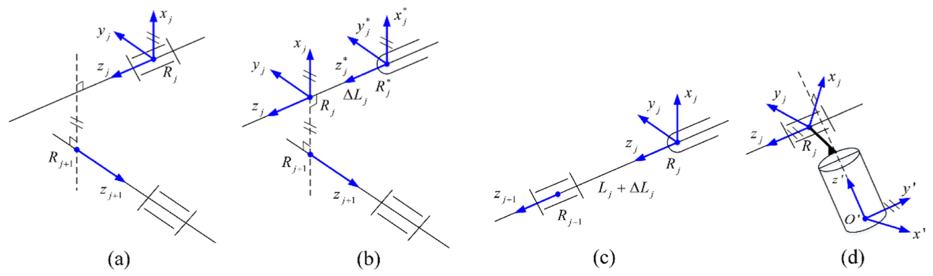
The definition of local frames with geometric errors: (a) when a R joint is followed by another R joint with axes not parallel, (b) when a P joint is followed by a R joint with axes not parallel, (c) when a P joint is followed by a R joint with axes collinear, and (d) when a R joint is followed by the end-effector.
Consequently,
where
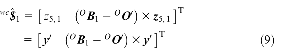
Because limb 1 is individually actuated by the P joint, the unit active wrench
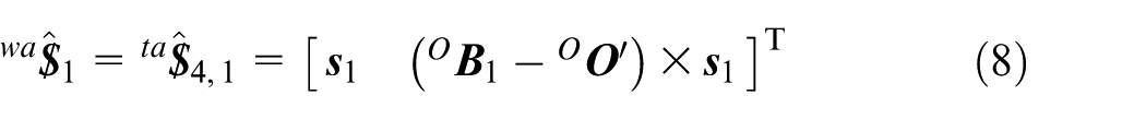
Besides, limb 1 has only 1-DoF constrained mobility, so the unit constrained wrench
Multiplying equation (7) by equations (8) and (9), respectively, results in
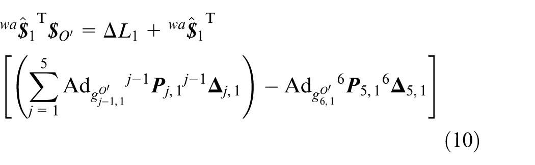
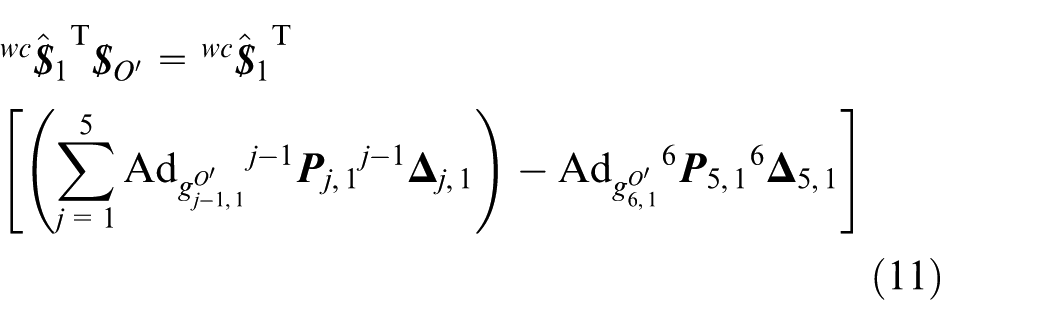
From Figure 2(b), it can be found that
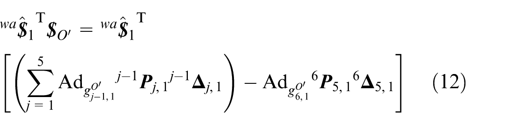
where
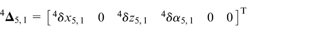
Then the error model of limb 1 can be developed by rearranging equations (11) and (12) in the matrix form
where
Error modeling for limb 2
Back to Figure 1(c), the joint constitution of limb 2 is divided into four divisions. To distinct the attached local frames in different divisions, they are also named in different ways. For division 1, there are
Similarly, the definitions of these local frames can also followed by the classification mentioned in section “Error modeling for limb 1”, then the pose error of the end-effector measured in
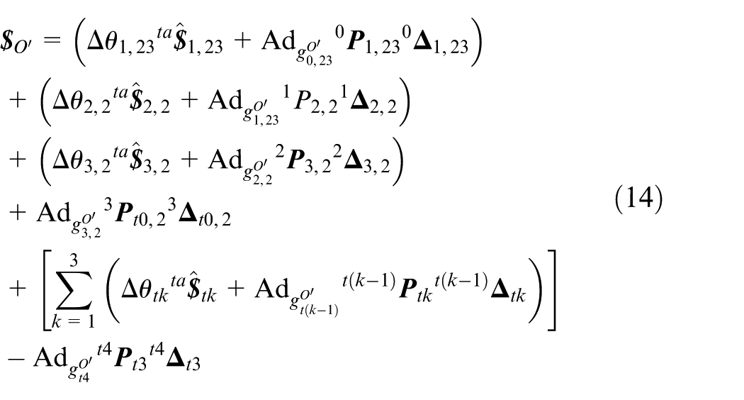
where, due to the planar constraint of limb 2, the geometric angle errors and parts of geometric length errors in division 2 and 3 are omitted, then
Subsequently, the unit active wrenches of link 2 and link 3 can be respectively expressed as
Multiplying equation (14) by equation (16) and equation (15) by equation (17) obtains
where
From Figure 2(c), it can be found that
where
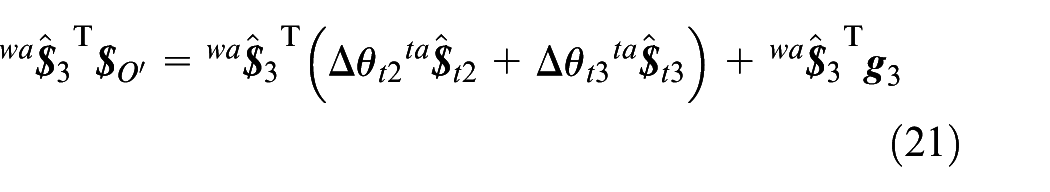
As it can be observed from equation (21), there are unknown terms
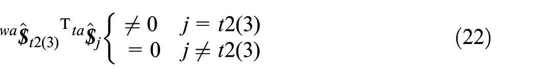
From the definition of
As shown in Figure 3, the correlated unit active wrenches can be obtained based on Blanding rules 6
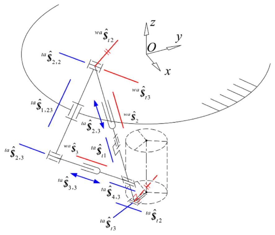
The unit twists and active wrenches in limb 2, where blue lines represent for rotational motion, blue arrows represent for translational motion, and red lines represent for constraint force.
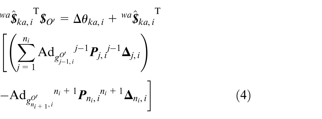
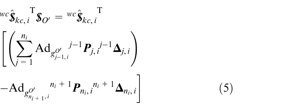
Multiplying equation (20) by equation (25) and equation (26), respectively, leads to
Thus,
Then the error model of limb 2 can be developed by rearranging equations (20) and (29) in the matrix form
where
Error modeling for the PKMT
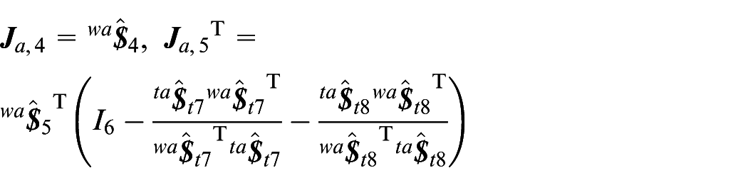
Since limb 3 is identical and arranged symmetrically with limb 2, error models of link 4 and link 5 can be easily deduced out from equation (30) through turning
where
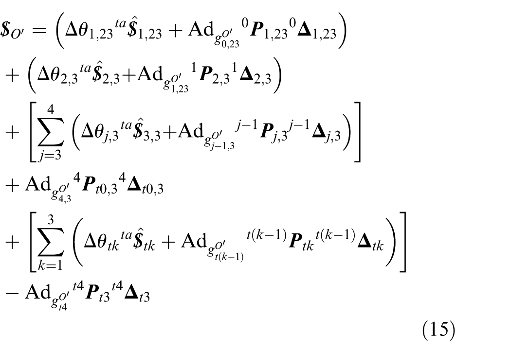
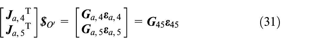
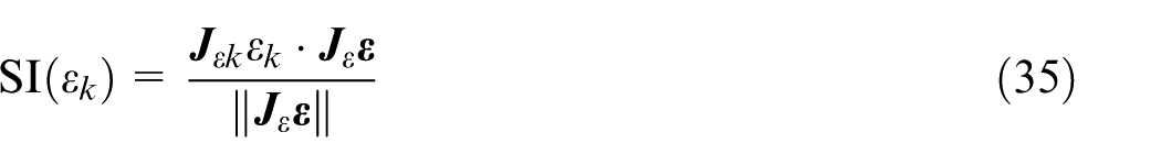
Uniting equations (14), (33), and (34) yields the error model of the PKMT

where
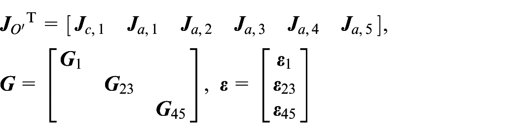
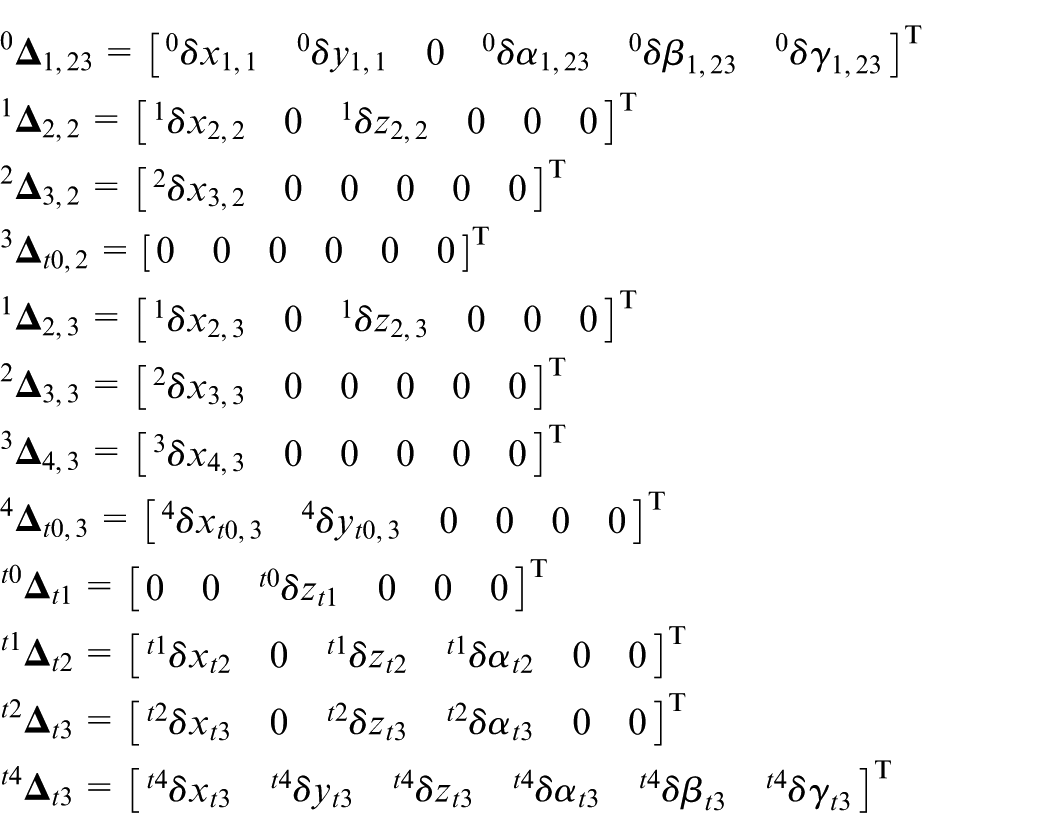
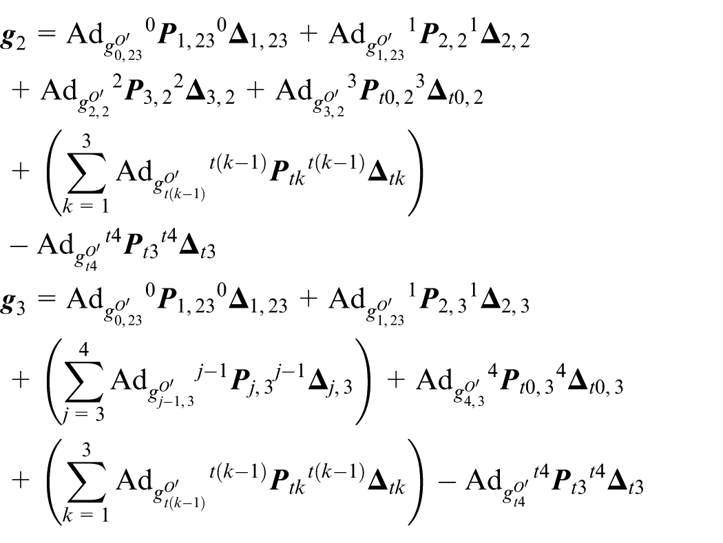
The detailed expressions of
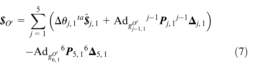
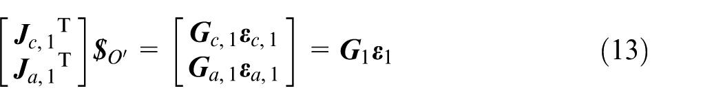
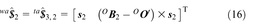
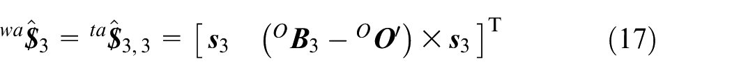
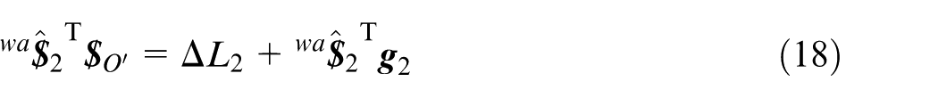
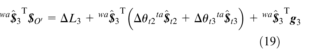
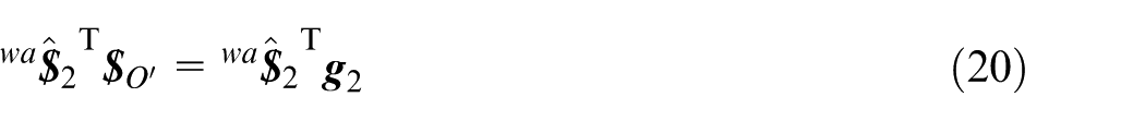
Multiplying

where
Sensitivity analysis
Definition of SIs
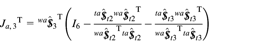
Concerning the effect of the single geometric error on the pose of the end-effector, equation (33) can be rewritten as
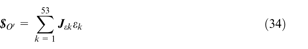
where
From equation (34), it can be known that
which embodies the effective contribution of
However, it is worth noting that the terms of
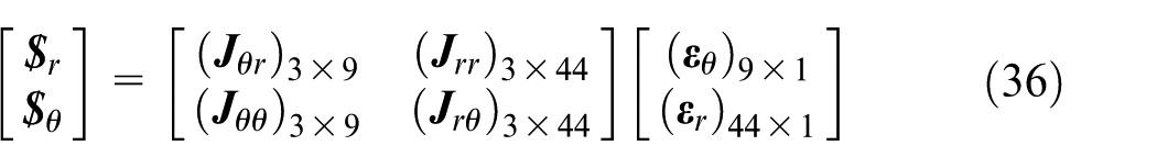
where
Due to varying with the pose of the end-effector, SIs are calculated at some specific pose, so they are actually local sensitivity indices (LSIs). Assuming that the values of elements in
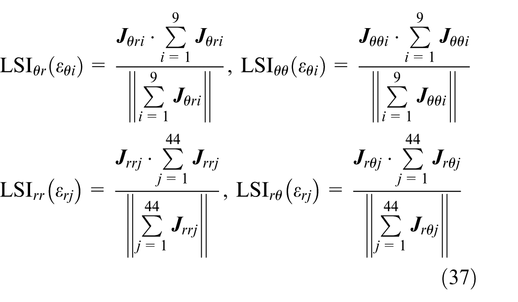
where
Usually, LSIs at plenty of poses should be collected to analyze the sensitivity of the pose error to each geometric error comprehensively. Based on the notion of mathematical statistics, global sensitivity indices (GSIs) and variable sensitivity indices (VSIs) are introduced in analogy with the mean value and standard deviation of LSIs, respectively
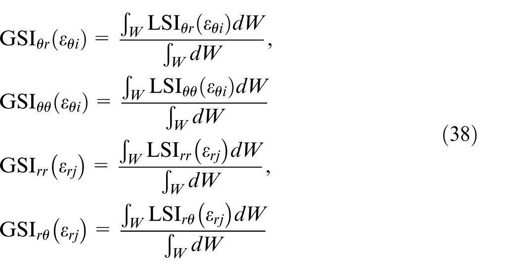
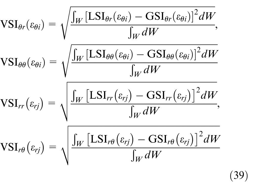
where W denotes the workspace of the PKM.
Because GSIs and VSIs independently reflect different data characteristics of LSIs, they had better be adopted to evaluate the influence on the pose error simultaneously. Thus, a kind of synthetic sensitivity indices (SSIs) is designed as
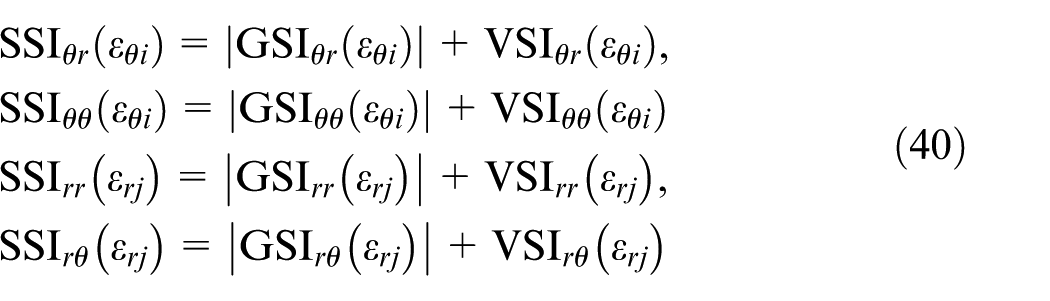
which uses the absolute average errors plus the average deviations to represent the average maximal impacts of each geometric error.
The next issue is to tell vital or trivial error sources among so many geometric errors from the achieved data of SSIs. Although there is no fixed standard, a consensus comes to that the vital errors are at least 10 times higher than the trivial ones. Hence, a kind of average sensitivity indices (ASIs) is defined as a baseline of evaluation criteria
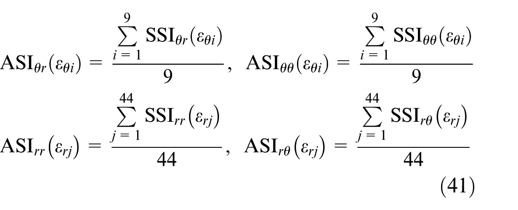
Then by designing a baseline factor
Sensitivity analysis for the PKMT
The nominal geometric parameters of the PKMT studied in this article are listed in Table 1. It is known that the end-effector of this PKMT can spatially realize 3-DoF translational positioning (
The nominal geometric parameters of the PKMT.
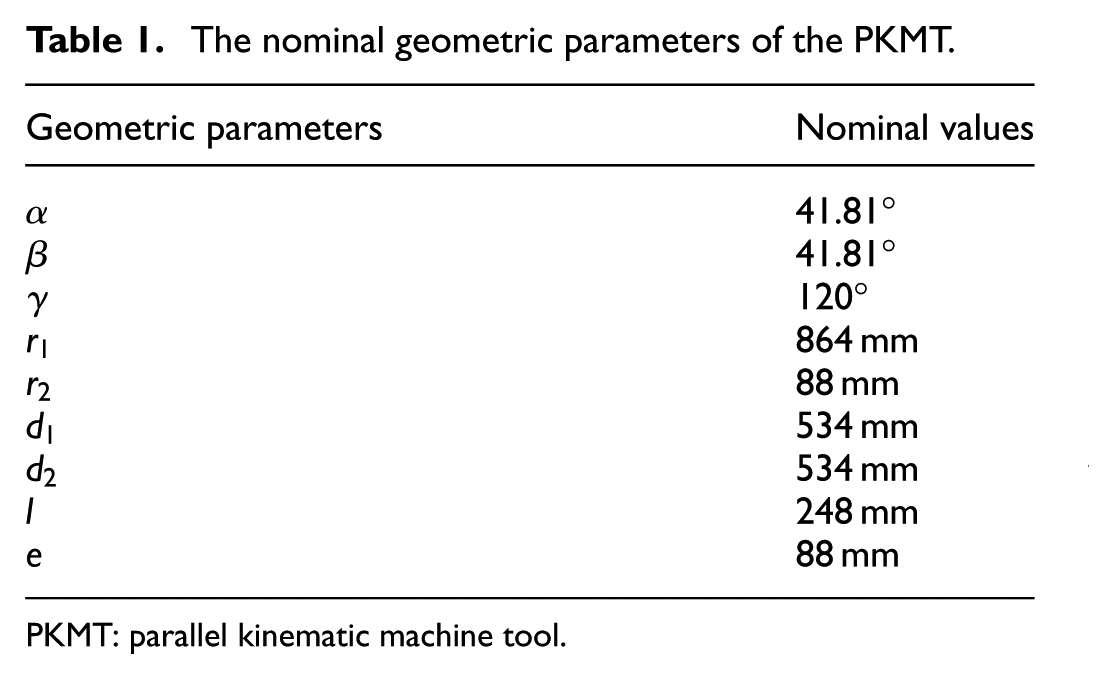
PKMT: parallel kinematic machine tool.
The workspace of the PKMT.
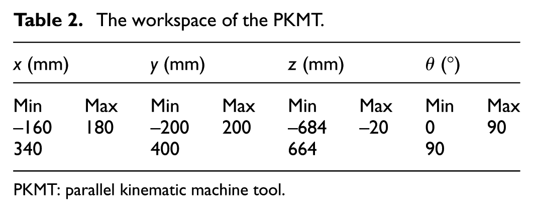
PKMT: parallel kinematic machine tool.
Via substituting the parameters from Tables 1 and 2 into equations (50)–(54), the results of sensitivity analysis are presented as histograms of SSIs in Figure 4. According to the abovementioned rules for choosing baseline factors in section “Definition of SIs”, a set of

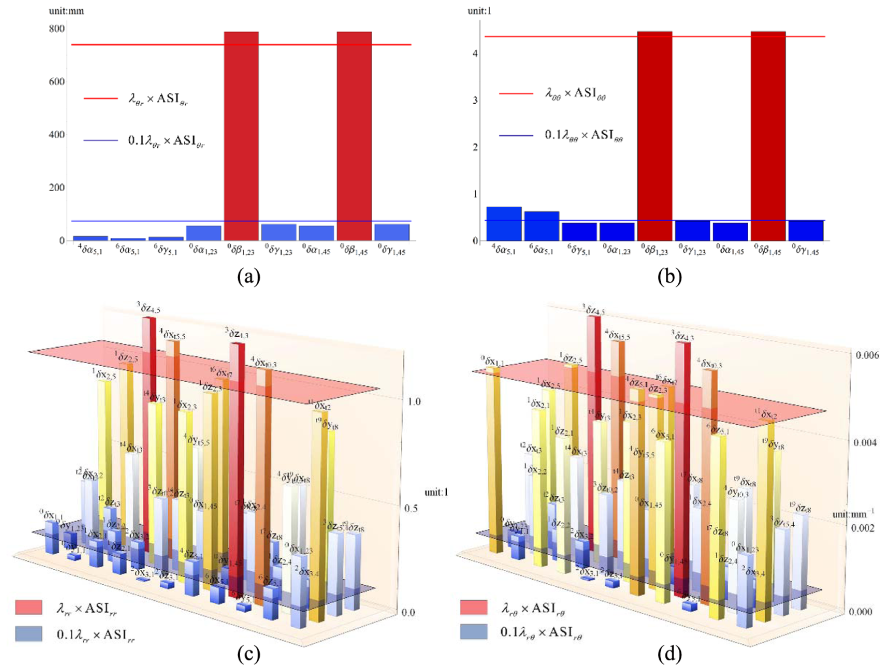
Histograms of the SSIs and corresponding baselines with respect to geometric errors: (a)
With the help of the baselines, some other conclusions can also be observed from Figure 4:
Figure 4(a) displays that
Figure 4(c) shows that
In summary, there are 10 geometric errors having striking impacts on the pose error of the end-effector, including two angle errors and eight length errors, which need strict restrictions when designing tolerances for manufacturing or assembly. Meanwhile, there are 10 geometric errors with tiny influence on the pose error of the end-effector, including five angle errors and five length errors, which can be deleted from the error model for simplification when carrying out kinematic calibration.
Simulating validation of sensitivity analysis results
Assuming that all the values of nine geometric angle errors are 0.1° and all the values of 44 geometric length errors are 0.1 mm, the pose errors of the end-effector can be calculated according to equation (37). Then the distributions of position errors (
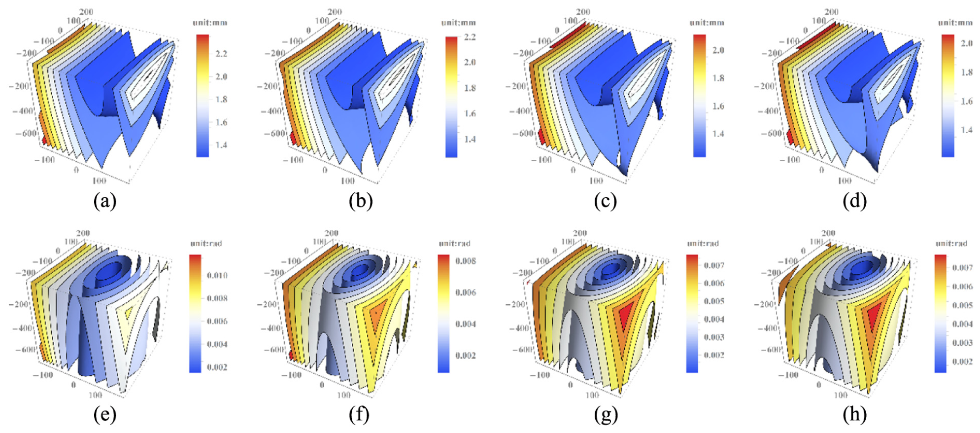
The position (a–d) and orientation (e–h) error distributions of the end-effector over the workspace without accuracy design: (a)
Based on sensitivity analysis, two numerical experiments of accuracy design are implemented via simulating the process of tolerance allocation with re-limiting the values of geometric errors. One is by modifying 10 trivial geometric errors to their one-tenth of the original values and the results are shown in Figure 6, which exhibits as nearly the same as Figure 5. The other one is by modifying 10 vital geometric errors to their one-tenth of the original values and the results are shown in Figure 7, which happen with great changes from Figure 5.
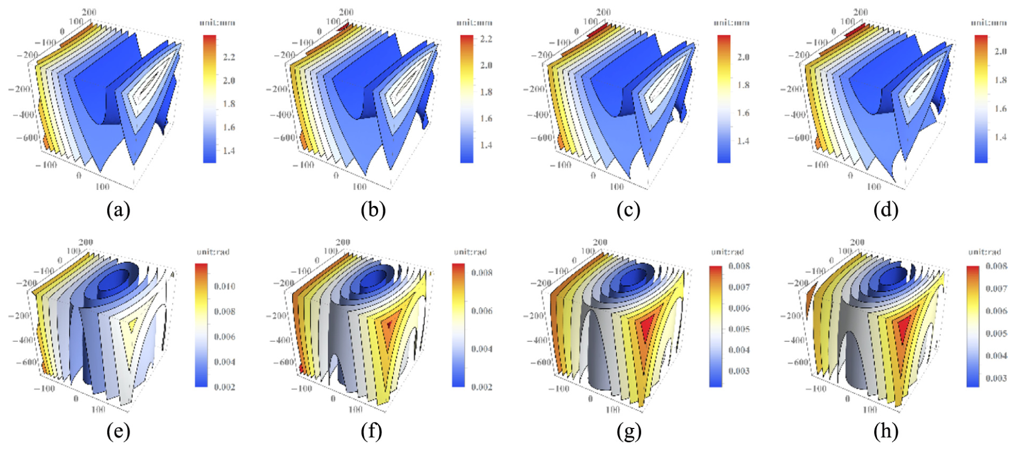
The position (a–d) and orientation (e–h) error distributions of the end-effector over the workspace with accuracy design of 10 trivial geometric errors: (a)
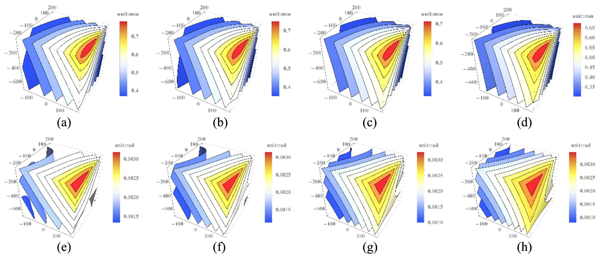
The position (a–d) and orientation (e–h) error distributions of the end-effector over the workspace with accuracy design of 10 vital geometric errors: (a)
To estimate the results explicitly, max and mean errors of (a) to (h) in Figures 5 to 7 are extracted, and comparisons are classified by units in Figure 8. From which, some conclusions can be observed as follows:
As for accuracy design of 10 trivial geometric errors, the largest decreasing ratios of max and mean position errors of the end-effector are −0.79% and −0.10%, respectively, with respect to the ones without accuracy design, while the largest decreasing ratios of max and mean orientation errors of the end-effector are 0.34% and −2.94%, respectively. As it can be seen that some pose errors of the end-effector deteriorate rather than improve by accuracy design, which indicates that some trivial geometric errors have contrary effects to other geometric errors, and embodies the vector property of geometric errors again.
As for accuracy design of 10 vital geometric errors, the smallest decreasing ratios of max and mean position errors of the end-effector are 65.56% and 72%, respectively, while the largest decreasing ratios reach 66.88% and 74.52%, respectively. In the meantime, the smallest decreasing ratios of max and mean orientation errors of the end-effector are 55.17% and 58%, respectively, while the largest decreasing ratios reach 73.75% and 59.68%, respectively.
In summary, the amount of vital and trivial geometric errors is the same as 10, which accounts for 18.87% of 53 in total. However, considerable improvements of the end-effector’s pose errors will take place when modifying vital errors other than trivial errors. Consequently, the correctness of sensitivity analysis can be verified.
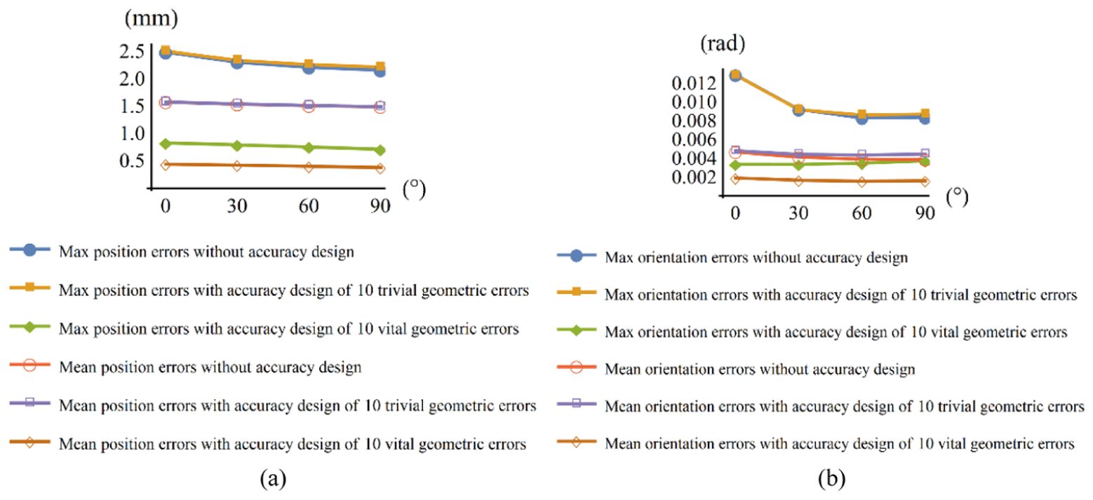
Comparisons of max and mean pose errors of the end-effector without/with accuracy design: (a) position errors and (b) orientation errors.
3D model validation of sensitivity analysis results
To validate the results of sensitivity analysis from the aspect of physical meaning, a 3D model with geometric errors are established with SolidWorks®. As shown in Figure 9(a) and (b), the original pose of the PKMT (
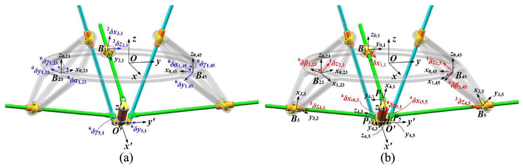
3D assemblies of the PKMT with (a) 10 trivial geometric errors (in blue) and (b) 10 vital geometric errors (in red).
The global coordinates of points
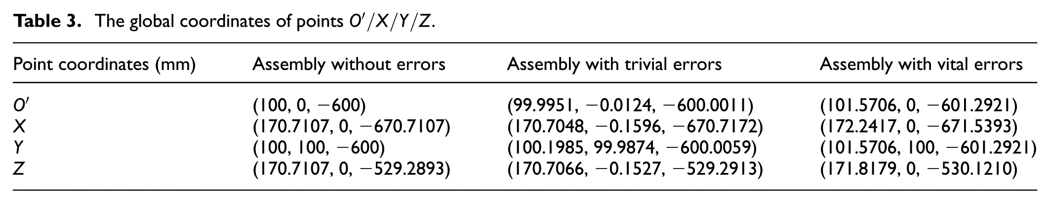
According to Table 3, the position and orientation errors are calculated as 0.0134 mm and 0.0020 rad, respectively, in the assembly with only trivial errors, while 2.0338 and 0.0048 rad, respectively, in the assembly with only vital errors, which are dramatically worse than the former when taken together. Since the chosen original pose is far from the limits of the workspace, it is somewhat representative, and the results of sensitivity analysis can be deduced to be correct.
Conclusion
Aiming at error modeling of a novel 5-DoF PKMT, a methodology based on screw theory is adopted because it can deal with the constraint characteristics of low-mobility PKMs and eliminate any unknown terms of passive joint motions. According to the EMJM of 53 geometric errors out of the developed error model of the PKMT, a set of SIs and baseline factors are designed for sensitivity analysis. Among them, LSIs are proposed based on the notion that geometric errors’ impacts embody vector properties on the end-effector’s pose errors, GSIs and VSIs are the mean value and standard deviation of LSIs data over the prescribed workspace, respectively, SSIs contain both data information of GSIs and VSIs, and ASIs and
Currently, the prototype of the PKMT is in the process of manufacturing, and the results of sensitivity analysis have been adopted. Meanwhile, the kinematic calibration of the prototype based on the results of this article is under study, and it will be presented in the future. Moreover, the whole procedure proposed in this article can also be extended to any other PKMs.
Footnotes
Appendix 1
Appendix 2
Appendix 3
Declaration of conflicting interests
The author(s) declared no potential conflicts of interest with respect to the research, authorship, and/or publication of this article.
Funding
The author(s) disclosed receipt of the following financial support for the research, authorship, and/or publication of this article: This work was supported by the National Natural Science Foundation of China (Grant No. 51675290 and No. 51425501). The second author wishes to acknowledge the support from the Alexander von Humboldt (AvH) Foundation.