
Abstract
The linear robot path is tangential and curvature discontinuity, which will lead to vibration and unnecessary hesitation during execution. Local corner transition method and local spline interpolation method are used in state-of-art industrial robot controller to reduce vibration, while local corner transition method cannot interpolate target points and local spline interpolation method cannot constrain chord errors. This research proposes a robot path local interpolation method that eliminates deficiencies of each method. The smoothing method satisfies all of the following requirements: G1 continuity, target point interpolation and chord tolerance confined, shape-preserving (free of self-intersection), and unified parameterization. The generated smooth path consists of linear path and circular arc path with G1 continuity. A geometric iterative method cooperating with local corner transition method is used to generate local interpolation path. Simulations and actual experiments verify the generated smooth path is G1 continuous, tolerance constrained, shape-preserving, and have high computational efficiency.
Introduction
Industrial robots are widely used in automotive and electrical/electronics industry. The continuity of robot path is important to robots’ execution accuracy and efficiency. In complex robotic applications, robot path is often generated by robot offline programming software, 1 formed of a series of short linear segments in Cartesian space. The linear path only has G0 continuity, which will cause unwanted vibrations, slow-downs, and low quality.2,3
Path smoothing algorithm can be used to generate continuous and tolerance constrained motions, thus to improve the efficiency and accuracy of robot application. A target point of linear robot path can be represented by a position in R3 (3-dimensional Euclidean space) and orientation in SO(3) (the group of all rotations in R3). 4 Both positions and orientations in Cartesian space are needed to be smoothed.
Position path smoothing methods
The smoothing methods in CNC machining or robotics for 3-dimensional paths can be divided into four classes: global interpolation method, global approximation method (fitting), local interpolation method, and local approximation methods (corner transition). 4
Global methods usually use splines to interpolate5,6 or approximate7,8 the whole set of data points. Global methods are often used offline because it is difficult to satisfy the requirements of interpolation, chord error constrained, and no self-intersection in real-time performance. PIA (Progressive iterative approximation methods),7,9 or the name of geometric iterative methods, are effective iterative methods used in global B-spline approximation or interpolation to avoid numerical instability. Deng and Lin 9 reported a 3D data fitting method of LSPIA (PIA for Least Squares). He et al. 7 used the ELSPIA (LSPIA method with energy term) to smooth three-axis tool path by cubic B-splines. Chord errors are always unconstrained because it is difficult to represent the chord error constraints analytically.
Local corner transition methods utilize a smooth curve to approximate linear path at corners. The method is popular in CNC tool path smoothing as the advantage of analytical computation. Zhao et al. 10 adopted a curvature-continuous B-spline to blend 3-axis linear tool path. Du et al. 11 used a cubic Bezier to smooth G01 paths under constraints of curvature variation energy. Li et al. 12 used the local transition scheme for a real-time and look-ahead interpolation of tool paths. Zhang et al. 13 proposed a corner smoothing method using feedrate blending under geometric and kinematic constraints. Similarly, the local corner transition methods were extended to five-axis tool path smoothing.14–18 In robotics, the parabolic path was commonly used for corner transition of position path.19,20 The reason is that trapezoidal speed planning can be easily realized by adopting the parabolic path. Also, quadratic Bezier path by Wang et al. 21 were designed in a SCARA robot control system. The local corner transition methods can generate smooth paths by simple calculation, but the smooth path cannot interpolate the target points.
Local spline interpolation methods utilize splines to interpolate target points considering adjacent path continuity. Fan et al. 22 used iterative methods to interpolate a three-axis tool path by Bezier curves. Fan et al. 23 proposed a chord error constrained and shape-preserving local interpolation method by adjusting undesired segments. Fleisig and Spence 24 used quintic polynomial splines to interpolate tool path with G2 continuity. The polynomial interpolation methods are also used in robotics3,25 to get target point interpolated smooth path. Zhao et al. 26 presented a NURBS curve interpolation method for a SCARA robot. Compared with local corner transition methods, local interpolation methods can generate smooth paths that interpolating target points, but the local interpolation methods are difficult to be solved analytically. High computation efficiency is an important requirement of local interpolation methods.
Orientation path smoothing methods
The orientation path of robots is often represented by quaternions, Euler angles or axis-angle method. 27 Linear orientation path is usually represented by SLERP (Spherical Linear Interpolation) curve. 20 The orientation path can be smoothed by the quaternion method. Kim and Nam 28 used circular blending quaternion curves to interpolate solid orientations. Then Kim and Nam 29 proposed a Hermite interpolation method using two circular quaternion curves on SO(3). Park and Ravani 30 generalized the concept of Bezier curves to Riemannian manifolds, which can be used for orientation interpolation. Furthermore, Kim et al. 31 presented a construction method of a C2-continuous B-spline quaternion curve which interpolates a sequence of orientations in SO(3).
The position path and orientation path can be smoothed separately using different parameters or smoothed synchronously using unified parameters. In five-axis machining, the tool tips and tool axes are synchronized using a third curve to fit the relationship between two parameters,6,14,24 or using the adjusting method in the smoothing process.5,8,32 Chen and Chen 33 proposed a synchronized fitting method for a six-axis machining robot manipulators, the orientation uses a rotation matrix and a vector to plan the tool orientations. However, the orientation errors cannot be constrained. He et al. 2 proposed a G2 continuous path interpolation method for SCARA robots, while the commercial robot control system does not accept user-defined splines.
Current commercial robot control systems provide local corner transition methods and local interpolation methods. ABB robotics 34 and KUKA robotics 35 use a distance to control the local corner transition shape. FANUC robotics 36 and YASKAWA Motoman robotics 37 use a scale parameter to specify the transition curve. YASKAWA Motoman robotics also provides a CR command to specify the radius of a transition arc. The two kinds of smoothing methods cannot satisfy the precision of target points and chord errors simultaneously. Moreover, the smoothing methods of orientation path are not specified in these methods.
About this research
The program path of SCARA robots can be represented by a position and a rotation angle of orientation, as the rotation axis of orientation is a constant value. This research uses a sequence of 4D points (a 3D position and a rotation angle) to represent SCARA robot path. Circular arc will be used as the smooth blending path, which has good properties of analytical arc length and curvature. The designed computational frame can be extended to smooth six-axis robot paths.
This research focuses on geometrical smoothing of robot path. This research aims to design a path smoothing method for SCARA robots. The smoothing methods can fulfill the requirements of G1 continuity, target points interpolation, chord error constrained, shape-preserving, and high computational efficiency. Moreover, the position path and orientation path are smoothed using unified parameters, no complicated parameter synchronization operation is required. A synchronized speeding planning method based on unified parameters of positions and orientations will be presented in next research.
This research is organized as follows. Section 2 presents the local arc transition method for SCARA robot path. The transit path is formulated by a convex combination formulation. Section 3 presents SCARA robot path interpolation method based on local arc transition. A geometric iterative method is used to calculate transition parameters. Section 4 presents several simulation experiments of the proposed method and comparisons with other methods. Section 5 is the actual experiments by drawing with a TURIN SCARA robot. At last, Section 6 concludes this research.
SCARA robot path local arc transition
The representation of SCARA linear robot path
In Cartesian space, a target point of linear robot path represents the position and orientation of Tool Coordinate System (TCS) relative to Robot base Coordinate System (RCS), as shown in Figure 1. The target points of SCARA robot path are represented by 4D point
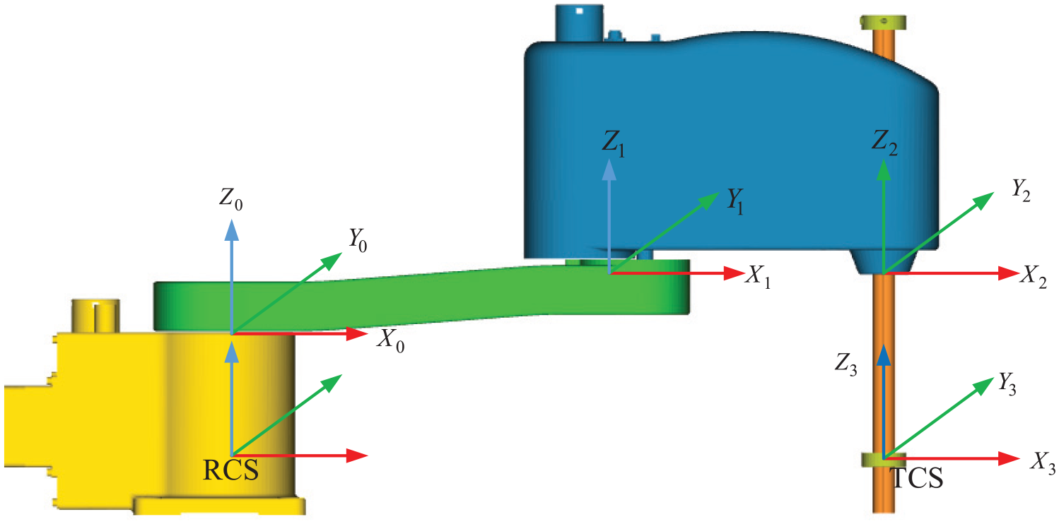
CAD model of a SCARA robot.
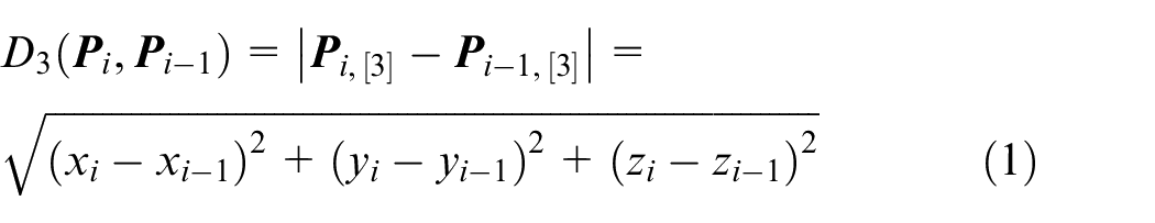
The distance between two 4D points can be defined by position distance and orientation distance. Suppose a 4D point is

Based on the definition of 4D representation and distance, a 4D arc path for SCARA robot path will be defined in Section 2.2.
Definition of a 4D circular arc path
A circular arc in R3 can be defined by the arc center, start point, end point and arc normal. Extend this definition to 4D space: suppose
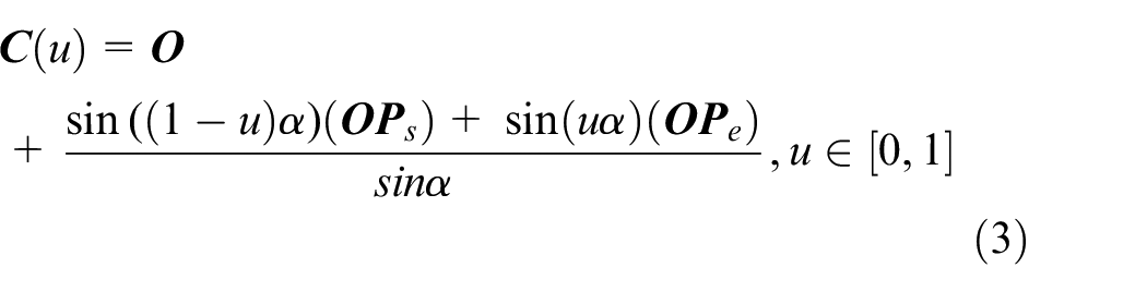
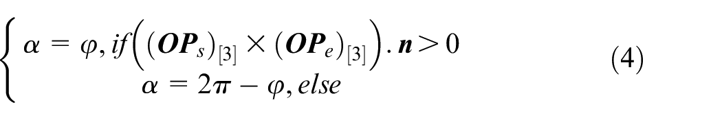
In equation (3),
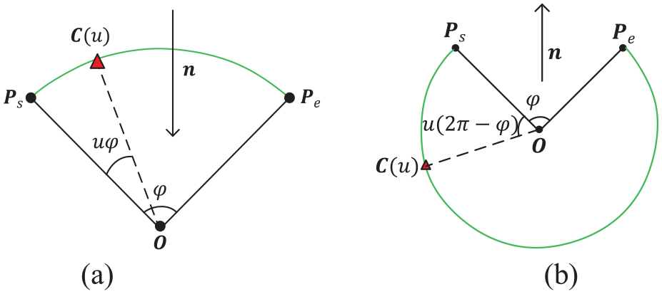
4D arc path: (a) minor arc and (b) major arc.
Using the unified parametrization, the position portion of 4D circular arc is a 3D arc, and the rotation portion is a continuous quadratic curve of rotation angles relative to rotation arc length.
Local arc transition and convex combination formulation
Circular arc in R3 is often used for corner smoothing, because its arc length and curvature can be analytically computed. This research will use 4D circular arcs to smooth linear SCARA robot path. Preliminary, local circular arc transition method is introduced.
As shown in Figure 3, considering three 4D points
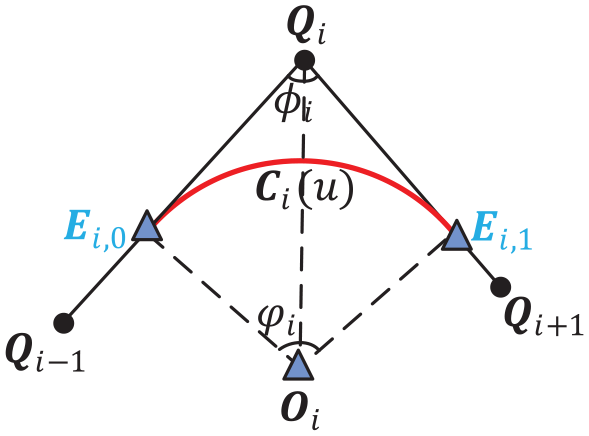
Local arc transition.
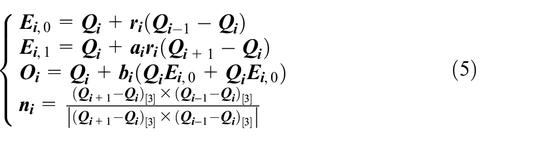
The arc transition curve can be built by equations (3)–(5) once the transition ratio
The following will use a simplified representation for the transition circular arc. By the theory of convex combination, the transition arc
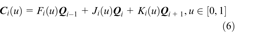
In which,
The convex combination based representation can simply computation and internal storage in this research, and the smoothing method can be easily extended to other transition curves.
Denoting

The parameter
The local arc transition method can be used to generate G1 continuous smooth path. To generate target point interpolation smooth path, this research will use an iterative method to construct a virtual linear path, and then use local arc transition method to get target point interpolated smooth path. The details will be introduced in Section 3.
SCARA robot path interpolation based on local arc transition
In this research, a geometric iterative method is used to generate virtual linear path (named pseudo path) and transition parameters, and then smooth path is constructed by the pseudo path and transition parameters using local arc transition. The smooth path should interpolate target points while satisfying chord tolerance constraints and free of self-intersection.
Algorithm overview
The illustration of the linear path, pseudo path, and smoothing path are shown in Figure 4(a). The first pseudo path
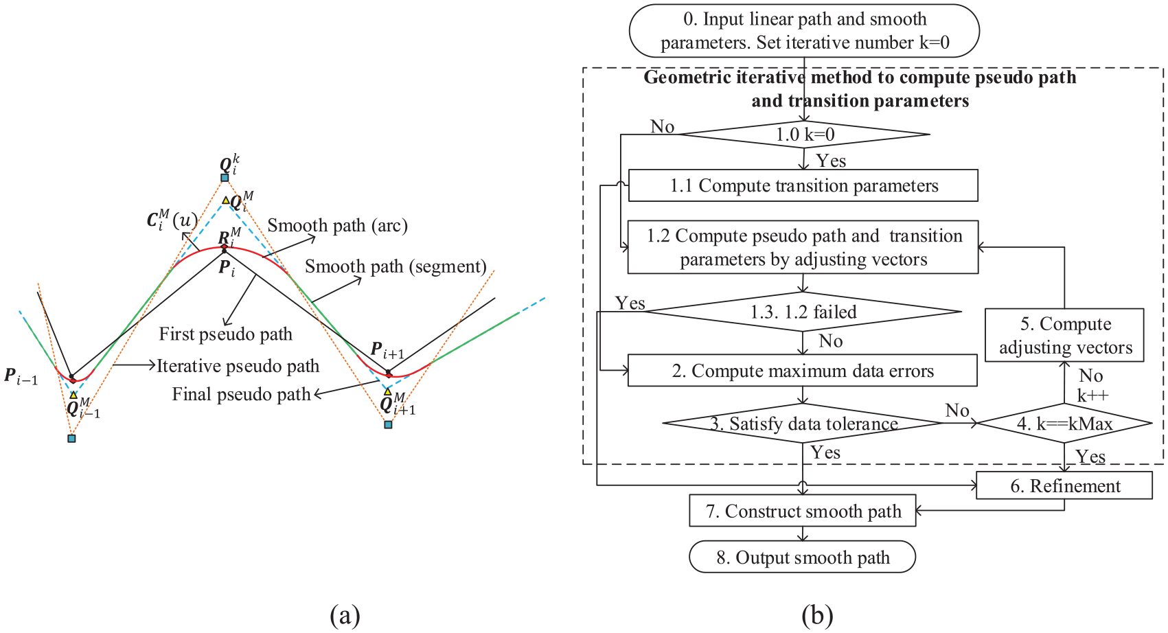
Illustration and flowchart of SCARA robot path smoothing method: (a) illustration of pseudo path and (b) flowchart of robot path smoothing.
The flowchart of the smoothing method is illustrating in Figure 4(b). First input linear path
Geometric iterative method for local arc interpolation
Except the G1 continuity requirement, the smoothing path should satisfy three other requirements: (1) Target points interpolation within given data point tolerance (include position data point tolerance and orientation data point tolerance). (2) Chord error confined within given chord tolerance. (3) Free of self-intersection by given shape-preserving parameters.
The requirements and objective function will be introduced in Section 3.2.1. The algorithm of computing pseudo path and transition parameters will be introduced in Section 3.2.2, and at last two adjusting vector selection methods are introduced in Section 3.2.3.
Requirements and objective function
Suppose the input linear path is
Suppose the constructed final pseudo path and transition parameters are
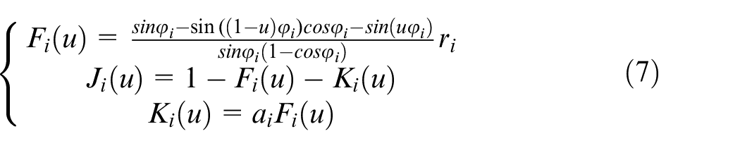
The interpolation requirements can be represented using equations (9) and (10).


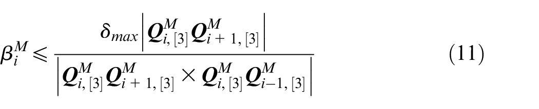
The position chord error around the i th corner can be developed by equation (11) as mentioned in He et al. 2 and Fan et al. 22
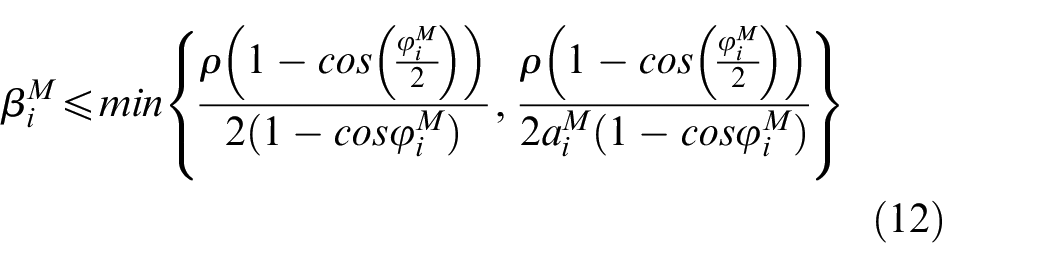
As for the shape-preserving constraint, as introduced in Huang et al.
17
a blank ratio
To reach the requirements of equations (9)–(12), a geometric iteration method is designed to update iterative pseudo path and transition parameter. In each iteration, a constrained optimization problem is built to compute iterative pseudo path and transition parameters.
Firstly, the objective function at the k th (
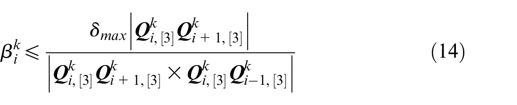
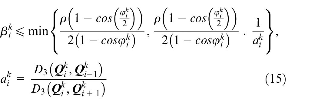
Then, the chord tolerance constraint and shape-preserving constraint are used to constrain
Furthermore, the iteration must be convergent for maximum position data error and maximum orientation data error, which means the k th data error at each target point should be smaller than the maximum data error at (
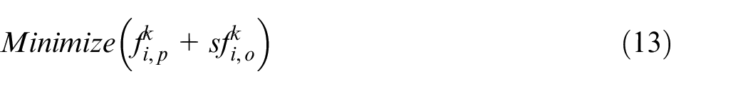
Based on the above analysis, a constrained optimization problem can be built for the i th target point in the k th iteration. The objection function is equation (13), under constraints of equations (14)–(17).


By derivation, the constrained optimization problem is a quadratic optimization problem of
Details of computing pseudo path and transition parameters
To solve the constrained optimization problem, the pseudo path in the k th iteration is updated by equation (18).

In which,
The range of
Adjusting vector selection and step range estimation
Based on the methods of LSPIA 9 and WPIA 38 with constant coefficient. This section proposes two adjusting vector selection methods.
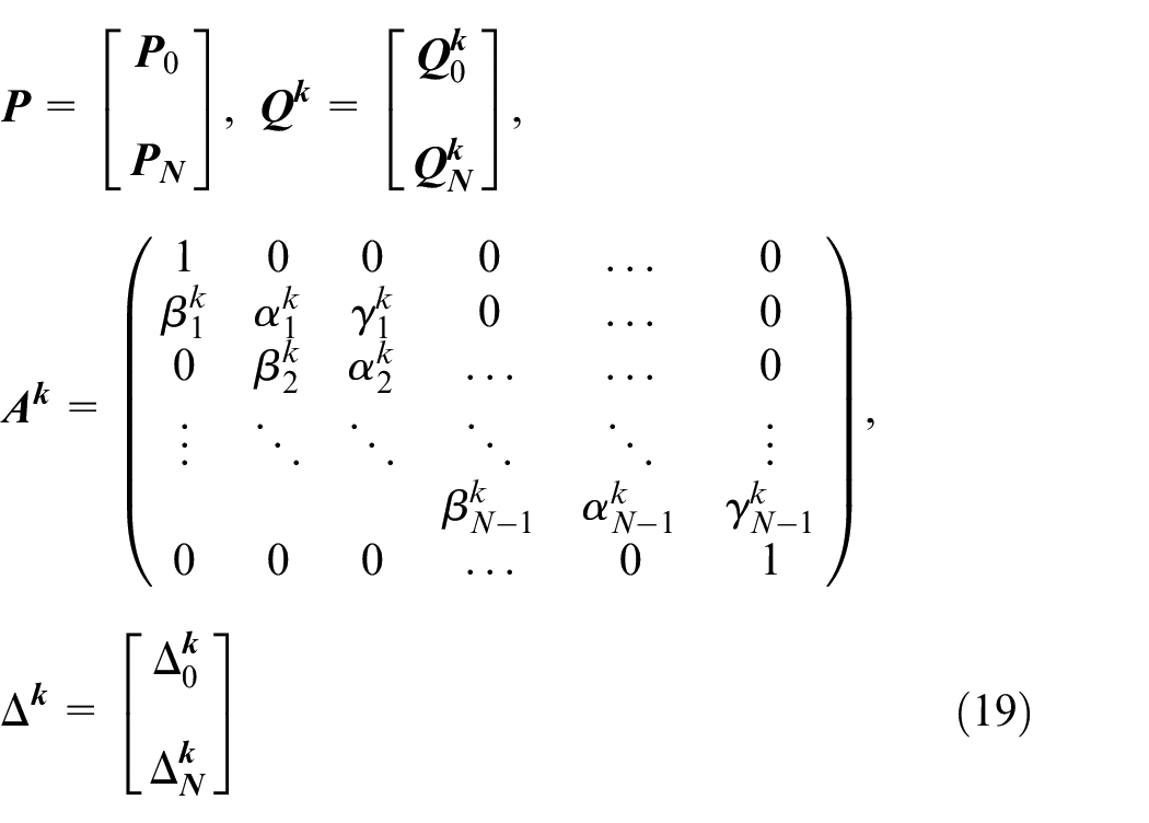
Equation (19) can be used to represent the target point
The first method is VCWPIA (Variable Coefficient Weighted Progressive Iterative Approximation).The adjusting vector can be represented by equation (20). The adjusting vector of VCWPIA considers the error vector of one target point, as shown in Figure 5(a).

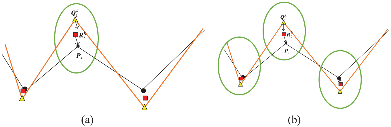
Adjusting vectors computation of VCWPIA and VCLSPIA: (a) VCWPIA method and (b) VCLSPIA method.
The second method is VCLSPIA (Variable Coefficient Least-Squares Progressive Iterative Approximation). The adjusting vector of VCLSPIA considers the error vector of adjacent three target points, which can be represented by equation (21). The diagram can be seen in Figure 5(b).
The range of step
For the two methods, the VCWPIA is prefer to be used as an interpolation method while VCLSPIA as an approximation method. An example is used to compare smoothing path generated by the two methods using same tolerance constraints.
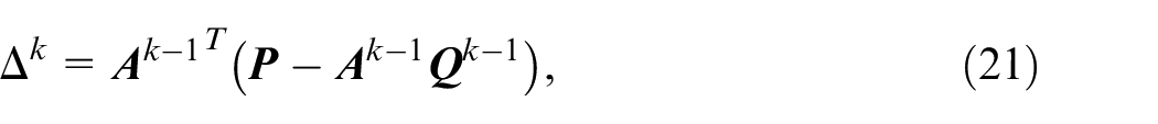
As shown in Figure 6, the input linear path has five target points. The position path using VCWPIA and VCLSPIA are illustrated in Figure 6(a), the rotation angle path relative to the parameter of position arc length are plotted in Figure 6(b). It demonstrates that the smooth path generated by VCLSPIA is closer to linear path than by VCWPIA.
Smoothing results comparison between VCWPIA and VCLSPIA: (a) position point path before and after robot path smoothing and (b) rotation angle path before and after robot path smoothing.
In the simulations of Section 4, the method of VCWPIA will be used, because under the same chord tolerance, the arc radius of position path by VCWPIA are bigger than by VCLSPIA, which can run faster with a smaller curvature.
Simulations
The proposed robot path smoothing method for SCARA robots is implemented in a self-developed software, using Visual Studio 2013, with a Window 8.1 Pro OS, 3.60 GHZ CPU and 16.0 GB memory. The figures are plotted in MATLAB R2014a. The linear robot paths are generated by a robot offline programming and simulation software “HiperMOS”. 39
In this section, the path before and after smoothing are illustrated and analyzed in Section 4.1. Then the smoothing method is compared with G1 smoothing results of Yaskawa Motoman robotics and ABB robotics.
SCARA robot path before and robot path smoothing
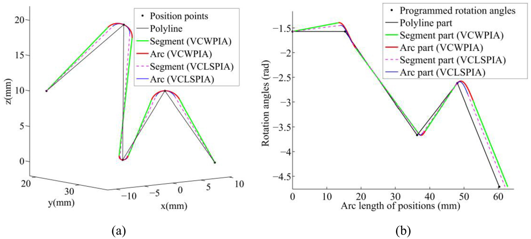
The path of a planar “dolphin” shaped model is generated by HiperMOS with 251 target points. The orientations are changed with the position path. In the smoothing algorithm, the position data point tolerance is set to 0.001 mm, the orientation data point tolerance is set to 1°, the chord tolerance is set to 0.1 mm. The shape-preserving parameter is set to
Figure 7 is the position paths before and after robot path smoothing. The linear robot path is plotted with black segments. The smooth robot path is consisting of segments (green lines) and arcs (red curves). It can be seen that the smooth position path has good smoothness and is shape-preserving.
Position robot path before and after smoothing: (a) overview, (b) marker A and (c) marker B.
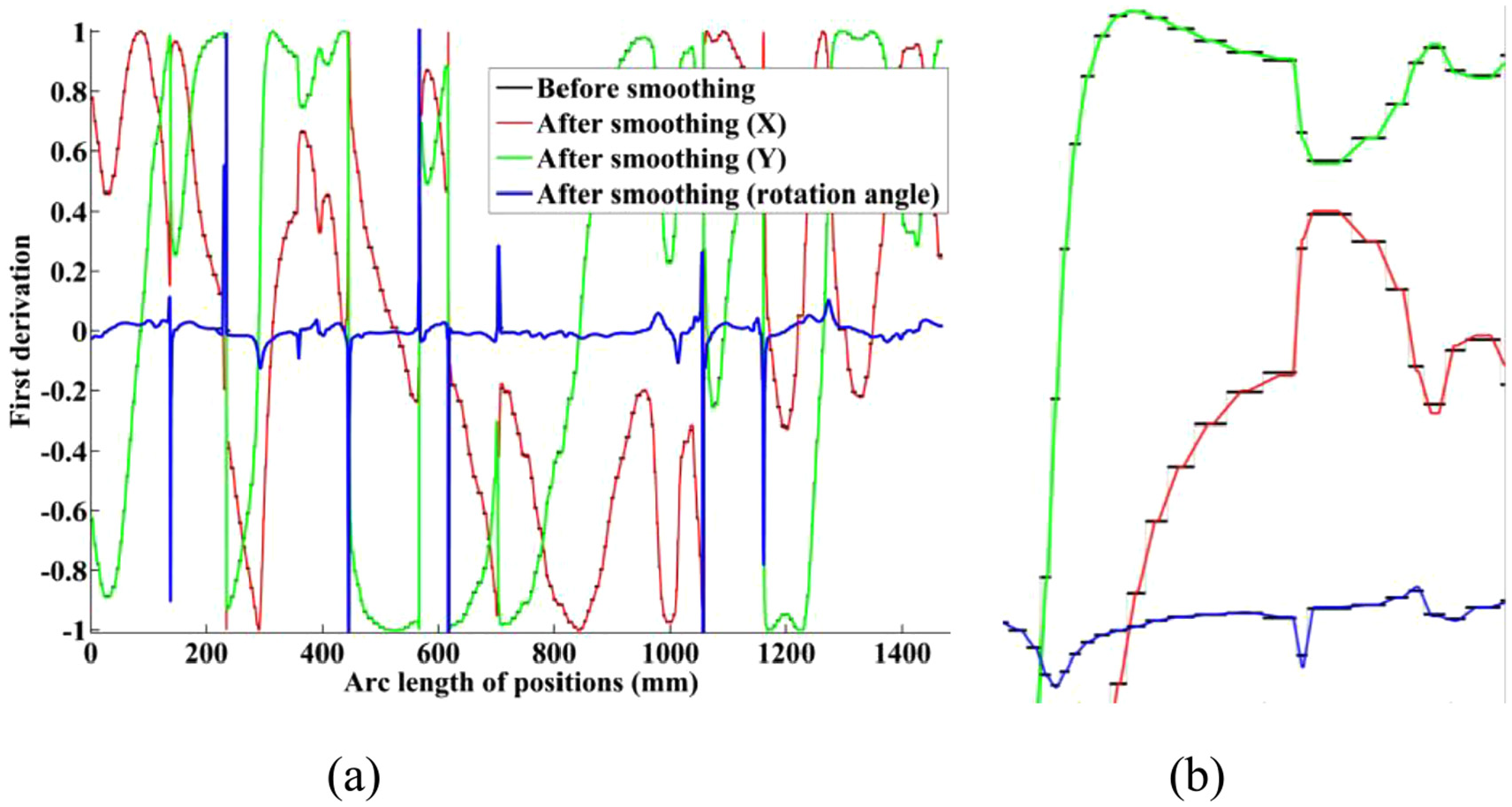
The rotation angle about position arc length after smoothing is G1 continuity. Figure 8 verifies the smoothness of rotation angles. Moreover, the first derivation of robot path about position arc length (
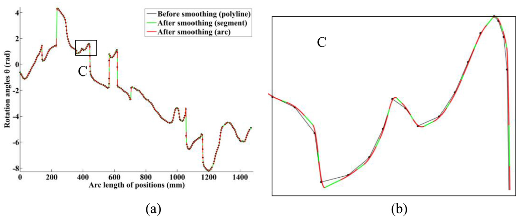
Rotation angles before and after smoothing: (a) overview and (b) amplified view around marker C.
First derivation about position path: (a) overview and (b) amplified view around marker D.
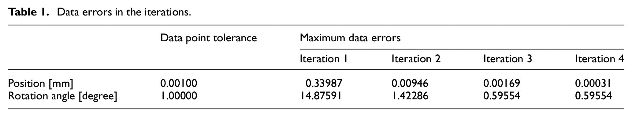
The data point tolerance is satisfied both for positions and rotation angles, which can be seen in Table 1. The maximum position data error and maximum orientation data error are both reduced in each iteration and reach the data point tolerance requirements at the fourth iteration.
Data errors in the iterations.
The actual position chord errors are plotted in Figure 10. The maximum chord error is 0.09998 mm, and the average chord error is 0.05057 mm. It can be seen that the smooth path is chord tolerance constrained.
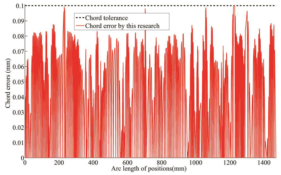
Chord tolerance and real chord errors.
The computational efficiency is estimated by Visual Studio 2013. The time of smoothing the 251 target points is 0.00162 s (average time for one point is 6.732e-6 s). It demonstrates that the proposed smoothing method has high computational efficiency, thus can be used for real-time motion control.
Comparison with smoothing method of Motoman
Yaskawa Motoman robotics use a code “CR” to approach linear path by local arc transition. The arc radius can be specified by the end-user. The simulation will compare the smoothing path generated by CR and by the proposed method.
A planar path of a character “Gong” is used. The position data point tolerance is set to 0.1 mm. The rotation angle tolerance is set to 1°. The chord tolerance is set to 3 mm. The CR is simulated run by the software MotoSimEG-VRC 5.2.
Figure 11(a) and (b) are the position path and orientation path generated by CR and by this research. The smooth path generated by the proposed method interpolates target points, while the smooth path by CR has target point data errors. Moreover, the rotation angles about position arc length of this research are smoother than of CR path.
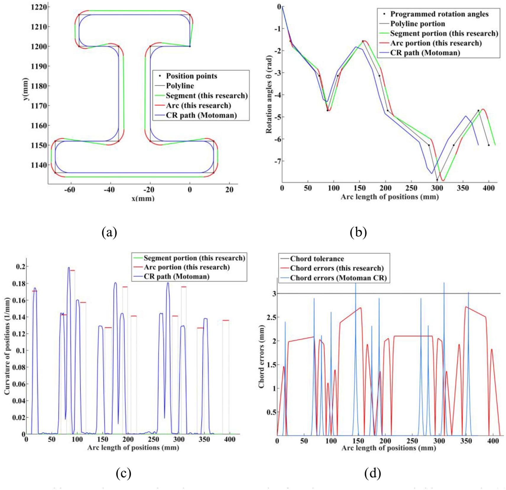
Smoothing results comparison between CR path of Yaskawa Motoman and this research: (a) position path comparison, (b) rotation angle path comparison, (c) curvature profiles, and (d) chord error profiles.
Figure 11(c) demonstrates the curvature profiles generated by this research are smoother by CR path. Moreover, by comparison of chord errors in Figure 11(d), the proposed smooth path is chord error confined, while the CR path is chord error uncontrolled by the end-user.
The comparison demonstrates that smooth path generated in this research is easy to control errors, and the rotation angle path is smoother than by CR code.
Comparison with smoothing method of ABB
ABB robotics uses a parabola curve to transit corners. The transition path is generated by specifying a transition level. 34 The real target point error cannot be constrained by the end-user directly. This section compares the smoothing results of ABB Z200 with smoothing results in this research.
A bigger character “Gong” is used. The smoothing parameters are set the same as the experiment in Section 4.2. The Z200 path is generated by simulation software RobotStudio 6.08 and a robot IRB910SC.
Figure 12(a) and (b) are the position path and rotation path generated by Z200 and this research. The smooth path generated by this research interpolates target points while Z200 path transits linear path at corners. Moreover, smooth path by this research is closer to the linear path than by ABB Z200 path.
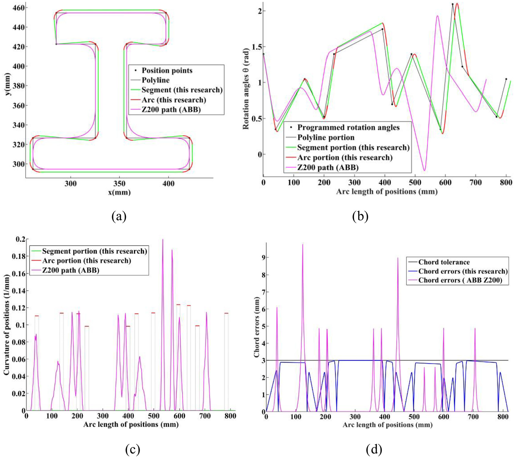
Smoothing results comparison between Z200 path of ABB and this research: (a) position path comparison, (b) rotation angle path comparison, (c) curvature profiles, and (d) chord error profiles.
Figure 12(c) is the comparison of curvature profile. It can be seen that curvature of smooth path by this research is more evenly and smaller than by Z200 path. The actual chord errors are computed and compared in Figure 12(d). It can be seen that chord errors of this research are confined by the tolerance 3 mm, while the maximum chord error of Z200 is 9.77634 mm. It demonstrates that the generated smooth path by this research has better accuracy and can be easier controlled by the end-user.
To summarize the above simulations, all the mentioned requirements are satisfied. Comparisons with smoothing methods of Motoman and ABB, the generated smooth paths by this research are smoother and tolerance constrained than other methods.
Experimental results
The generated G1 smooth path is actually verified by drawing through a SCARA robot. Three types of robot path (the linear path, the corner transition path generated by the robot controller, and the G1 smooth path generated by this research) are drawing together in the experiments. The drawing results and actual errors are compared.
Experiment platform
A “Heart” shaped planar linear path with nine target point is designed in the offline programming software “HiperMOS”. To smooth the linear path, the position data point tolerance is set to 0.01 mm, and the chord tolerance is set to 2 mm. The orientation is not changed in the experiment.
The linear path and G1 smooth path are simulated in software HiperMOS with a TURIN SCARA robot (STH030S/E-3KG-600 mm). Figure 13(a) is the illustration of the SCARA robot and G1 smooth path in HiperMOS. Figure 13(b) is the actual SCARA robot and the setup of drawing. A pen is installed on the end effector of robot by a clamp. A piece of A4 paper is fixed in the work table.
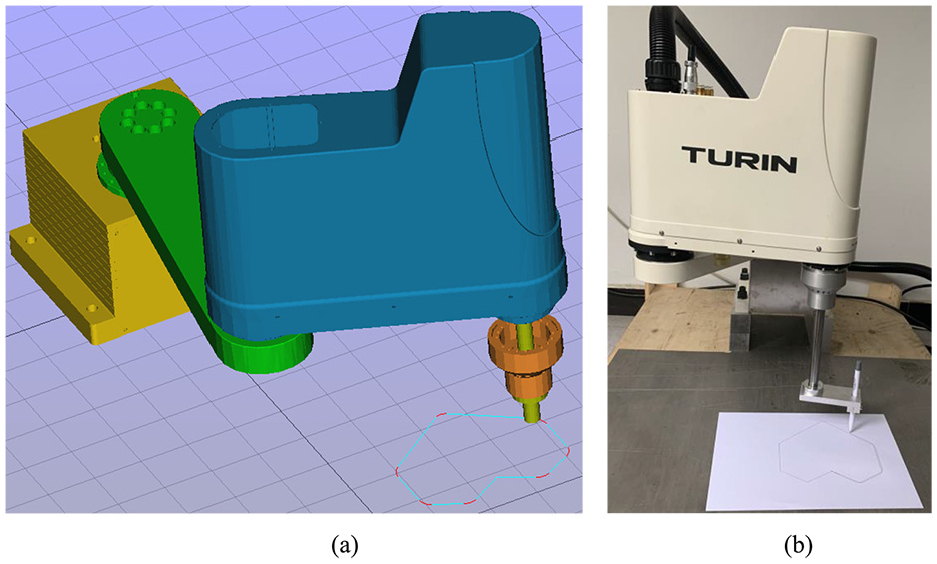
Drawing by a SCARA robot: (a) simulation in HiperMOS and (b) actual running.
Experiment results
The three types of path are drawn by three different color of pens. Firstly, the linear path is drawn by a black pen, then the corner transition path generated by TURIN robot controller is drawn by a blue pen, at last the G1 smooth path is drawn by a red pen. Two drawings are presented in Figure 14, corresponding to experiments performed for two different speed settings of robot.
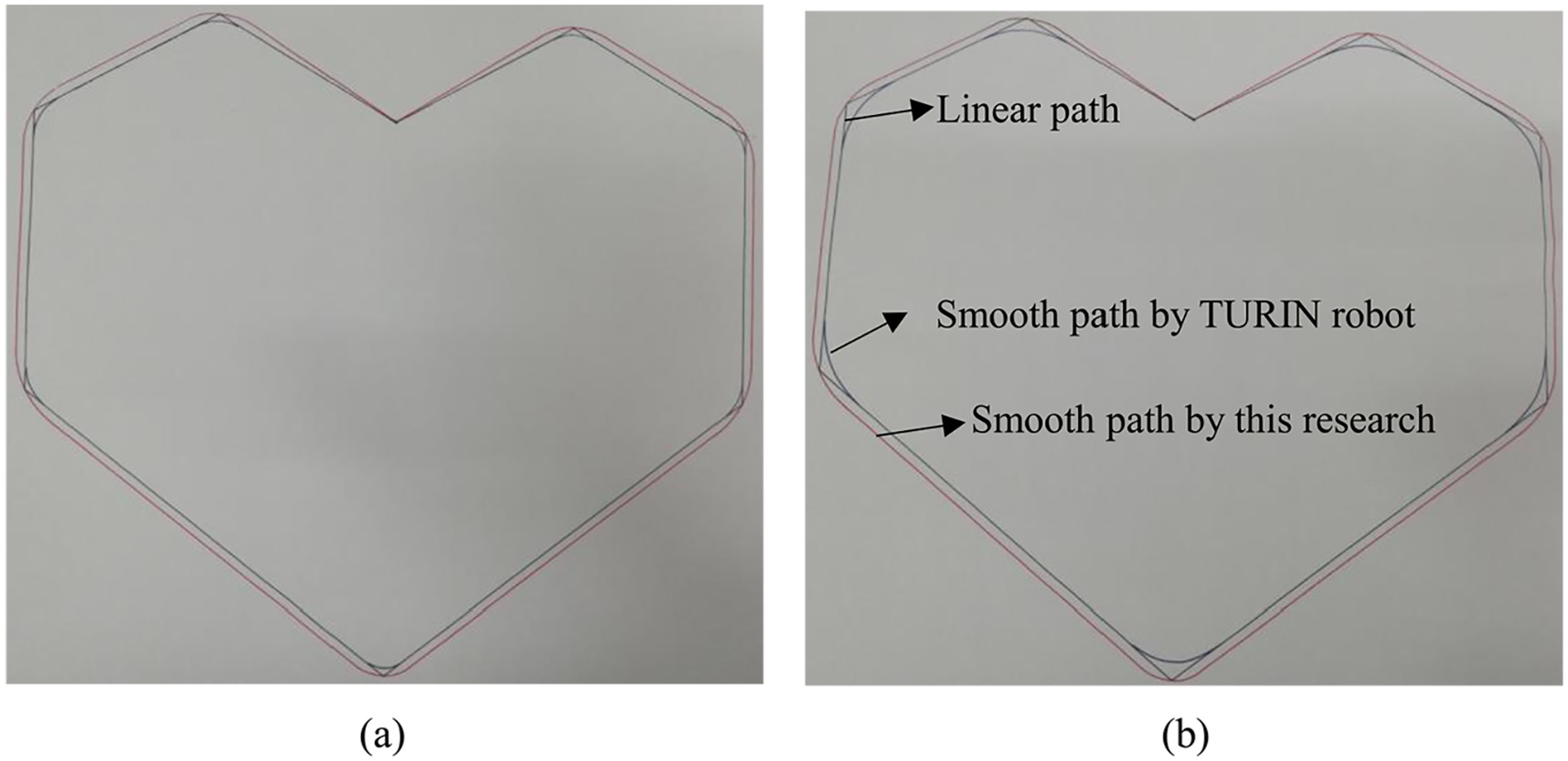
Three types of path by robot drawing: (a) first experiment and (b) second experiment.
A first experiment is designed with speed of 40 mm/s, and the acceleration of 200 mm/s2. The corner transition path is generated by robot controller with maximum transition. The drawing results of three types of path are shown in Figure 14(a). It can be seen that the blue transition path do not interpolate the target points. By measurement, the position error is about 1 mm. while the red G1 smooth path interpolates the targets points under the chord tolerance of 2 mm. It demonstrates that the resulting path has advantage of target point interpolation and chord errors constrained.
A second experiment is designed with speed of 80 mm/s, and the acceleration of 400 mm/s2. The corner transition path is generated by the same method with the first experiment. Figure 14(b) presents the drawing results of three types of path. It can be seen that the transition path changes transition shape with the change of speed and acceleration. By measurement, the position error is about 3 mm. However, the red G1 smooth path has same shape as in the first experiments.
The two experiments show the advantage of the smooth path relative to corner transition path of TURIN robot controller, i.e. easy-controlled tolerance and unchanged shape with different speed. It indicates that the G1 smooth path is fit for precision-demanding application.
Conclusion
This research optimizes any given SCARA linear robot path to achieve
Simulations and experiments demonstrate the effectiveness of the proposed SCARA robot path arc interpolation. Comparison with similar methods demonstrates the proposed method can generate smoother path while satisfying all the requirements.
At the consideration of future work, the proposed method will be used for six-axis robot path smoothing.
Footnotes
Appendix
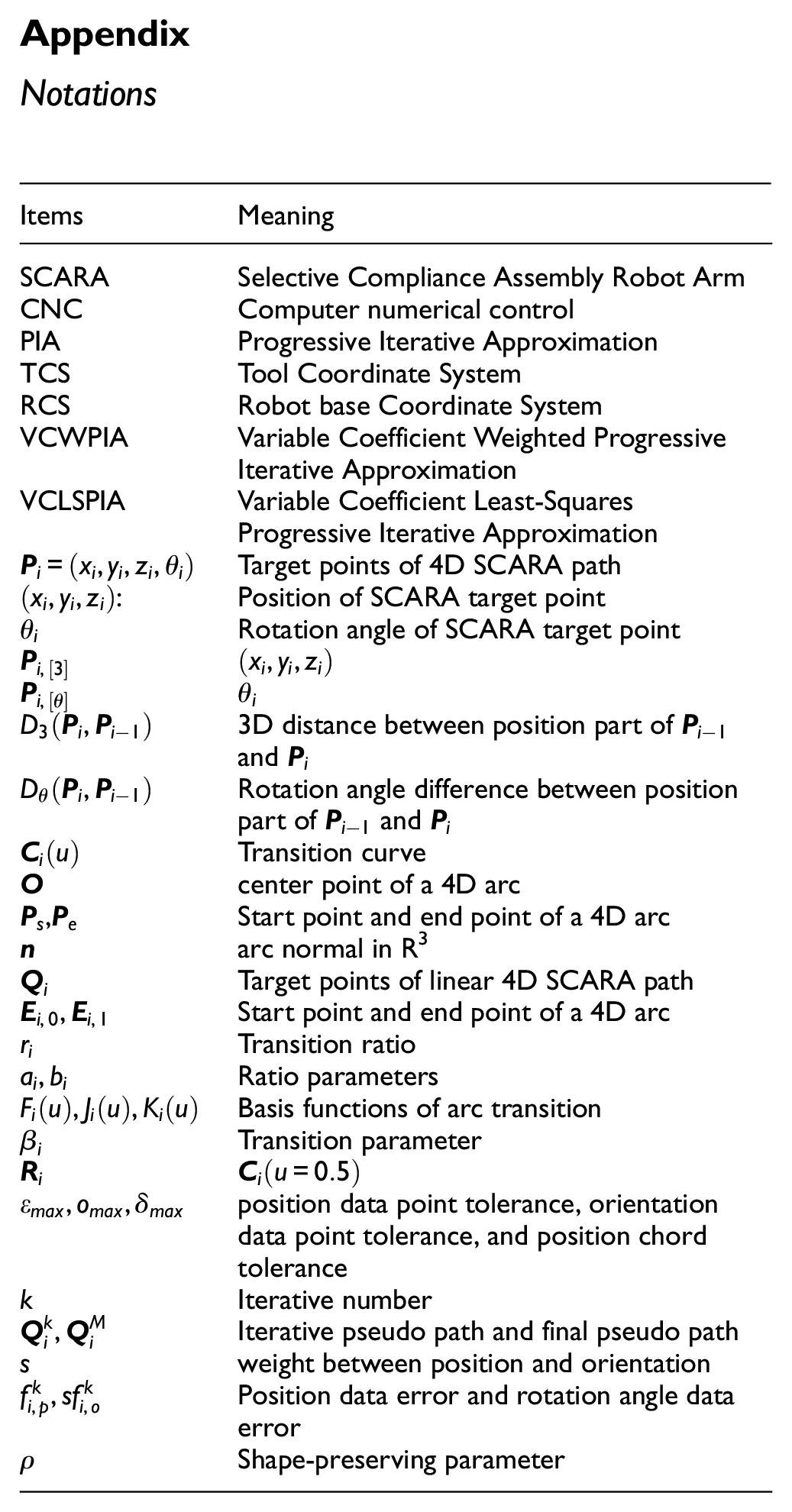
Notations
| Items | Meaning |
|---|---|
| SCARA | Selective Compliance Assembly Robot Arm |
| CNC | Computer numerical control |
| PIA | Progressive Iterative Approximation |
| TCS | Tool Coordinate System |
| RCS | Robot base Coordinate System |
| VCWPIA | Variable Coefficient Weighted Progressive Iterative Approximation |
| VCLSPIA | Variable Coefficient Least-Squares Progressive Iterative Approximation |
| Target points of 4D SCARA path | |
| : | Position of SCARA target point |
| Rotation angle of SCARA target point | |
| 3D distance between position part of and | |
| Rotation angle difference between position part of and | |
| Transition curve | |
| center point of a 4D arc | |
| , | Start point and end point of a 4D arc |
| arc normal in R3 | |
| Target points of linear 4D SCARA path | |
| Start point and end point of a 4D arc | |
| Transition ratio | |
| Ratio parameters | |
| Basis functions of arc transition | |
| Transition parameter | |
| position data point tolerance, orientation data point tolerance, and position chord tolerance | |
| k | Iterative number |
| Iterative pseudo path and final pseudo path | |
| s | weight between position and orientation |
| Position data error and rotation angle data error | |
| Shape-preserving parameter |
Declaration of conflicting interests
The author(s) declared no potential conflicts of interest with respect to the research, authorship, and/or publication of this article.
Funding
The author(s) disclosed receipt of the following financial support for the research, authorship, and/or publication of this article: This work was supported by the National Natural Science Foundation of China [51575386].