
Abstract
Many existing tolerancing models deal with the tolerance analysis of mechanical assemblies using linear stack-up function, which will cause truncation errors for nonlinear assembly problem. This article proposes a new method for describing the variation propagation based on the product of exponentials formula. Both the length deviations and the angle deviations are uniformly represented by twist coordinates. Accordingly, the nonlinear stack-up functions relating the assembly functional requirements to the manufacturing variations can be derived, and no truncation errors generated. A three-dimensional assembly case is studied exploiting the proposed method and the direct linearization method, respectively. It appears that the product of exponentials formula can bring consistent tolerance analysis results with the exact geometric solutions, whereas there are some small errors in the analysis results of direct linearization method. The precision of tolerance estimation via the product of exponentials formula is improved by 0.52% at the most compared with that by the direct linearization method. Due to the elimination of local datum reference frames, the product of exponentials formula can also lead to a more concise description of tolerance accumulation than the direct linearization method.
Introduction
Tolerances define tolerable variations in dimension, geometry and position of part in a mechanical product. Unreasonable part tolerances may lead to serious assembly difficulties and even unacceptable loss of functional quality. Therefore, it is very necessary to perform the tolerance analysis in mechanical design to evaluate the effects due to the tolerances of parts on the functional requirements of the assembly.
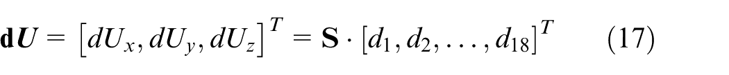
For analysis of each assembly functional requirement, a stack-up function revealing the accumulation of variations in the assembly should be built.1,2 In general, the most traditional method to build a stack-up function is linearizing the assembly response function which is normally an explicit constraint equation describing the relations between the input component variables and the output assembly variable.3–6 The linearization (the first-order Taylor’s series expansion) will lead to a constant sensitivity matrix
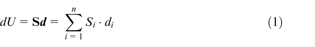
where dU denotes the assembly variation, and
There are still some other tolerance analysis methods which can directly derive the stack-up functions without resorting to the assembly response function, as have been discussed by many literatures.14–17 The Jacobian model 18 uses kinematic chains composed of functional elements to represent the stack of dimensions and variations. The Torsor model19,20 describes the three-dimensional (3D) tolerance zones by small displacement screws. The two models are further combined to form the unified Jacobian–Torsor model. 21 The Variational model1,22 employs homogeneous transformation matrix to express the variations in an assembly. The Matrix model 23 uses displacement matrix to describe the small displacements of a feature within the tolerance zone. Recently, a new method based on the free-body diagrams of force analysis was proposed for calculating the sensitivities of a two-dimensional (2D) assembly. 9 Although the representations of individual variations and tolerance accumulation in these methods are different, the resulting stack-up functions are mostly linear14–16 and can be written in the form of formula (1).
In fact, the linear stack-up function derived using many existing tolerance analysis models is an approximation to the 2D/3D assembly system. 8 If the assembly has strong nonlinearity, or if the component tolerances are not small enough compared with their nominal dimensions, the linear mapping from the individual variations to the assembly variation may cause serious truncation errors and then reduce the accuracy of tolerance analysis.3,8,24 Besides, the DLM, Jacobian, Torsor, Variational and Matrix are required to attach local datum reference frame (DRF) to each vector or feature, which may make it troublesome when tackling the problem of tolerance analysis for a complex 3D assembly. Some methods such as the Matrix and Torsor have also been indicated to be powerless in the analysis of statistical variations.14,15
In this article, a new method termed the product of exponentials (POE) formula is introduced to perform the tolerance analysis of mechanical assemblies. The individual variations and variation propagations are, respectively, described by the twist coordinates and exponential maps. The formula was originally used to model the forward kinematics of robot manipulators 25 and has attracted much attention in the parameters calibration of robotics over the past few years.26–29 However, in the field of assembly, so far we have not found the reports using the POE formula to perform the tolerance analysis. The primary advantages of the POE formula lie in the smooth description of fluctuations of kinematic parameters with changes in joint axes and the uniform representation of translation and rotation.26,28,29 Therefore, the description of mechanical assembly based on the POE formula, may bring an analytic and nonlinear stack-up function which can directly reveal the relations between the component variations and the assembly functional requirements. Consequently, the precision of tolerance analysis can be enhanced especially for a 3D complicated assembly. In addition, the POE formula is a zero reference position description,26,28 which means the method is suitable for integration with commercial computer-aided design (CAD) system to form the computer-aided tolerancing.
The article is organized as follows: section “Tolerance analysis based on the POE formula” provides a mathematic description on the individual variations and variation propagation via the POE formula. Next, a 3D assembly case is studied to verify the feasibility and advantages of the POE formula in tolerance analysis. The conclusions are drawn in the last section.
Tolerance analysis based on the POE formula
The parameterization of individual variation
The tolerance analysis via the POE formula depends on the vector-loop-based assembly model, in which the component dimensions and assembly dimensions are all represented by vectors, and the assembly constraints are described by kinematic joints at the mating part interfaces.10,11 The vectors are arranged in chains representing those dimensions that stack together to determine the resultant assembly dimensions. 16 In the assembly vector loop, each vector embodies the translation and rotation relative to the previous vector. Therefore, there are two kinds of variation sources, one is the length deviation depicting the fluctuation of length dimension and clearance between mating parts and the other is the angle deviation which expresses the change appearing in the interactive orientation relationships. The two variations should be considered to form a complete model of assembly variation.
Create the global DRF for the assembly vector loop. The individual variations can be mathematically described by screw motion. Without the loss of generality, the direction and location of both the length deviation and the angle deviation are jointly expressed by a twist of
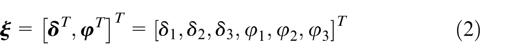
where
More specifically, the length deviation only leads to a translation of the component variable, so that
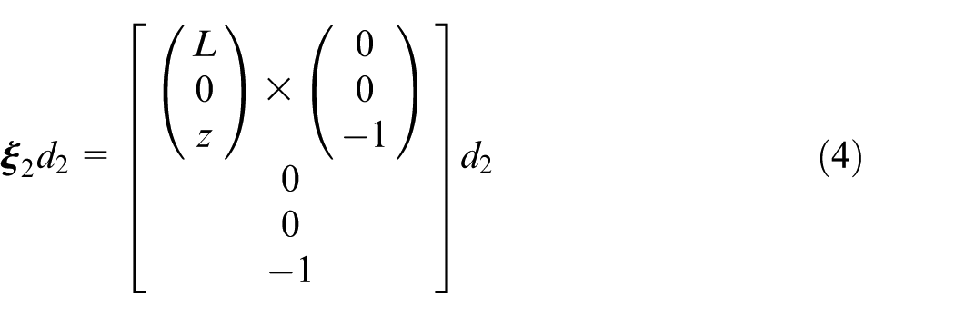
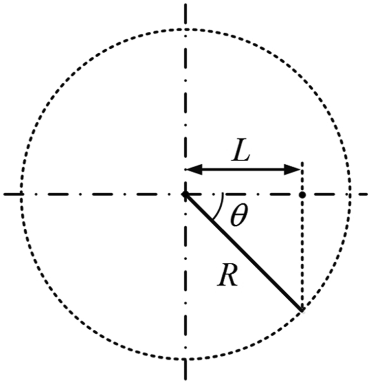
To illustrate the definitions more clearly, a general part with 2 dimensional variations is presented in Figure 1. R is a reference point settled at the origin of global DRF and is supposed to be fixed with the line AB. Since ΔL is a length deviation along the direction of

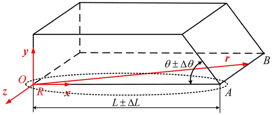
A simple part with two dimensional variations.
where
where
It is easy to divide the dimensional tolerances into length and angle deviations. In contrast, the geometric feature tolerances classified into five groups, that is, form, orientation, profile, position and run-out according to the standards of ISO 1101:2012(en) 30 and ASME Y14.5M:2009 31 are relatively sophisticated. As the tolerance analysis models are varied, the corresponding treatments to geometric tolerances are different. 32 In the vector-loop-based tolerance analysis model, the geometric variation is considered as special dimensional variation with zero nominal value that is placed at the contact point between mating parts. Moreover, the tolerance associated with each joint may result in an independent translation or rotation or both.12,17,32 In other words, the geometric feature tolerances can be equivalent to the combinations of angle and length deviations. Since the geometric tolerances have a lot of forms, the detailed treatment for each of them is not studied in this article.
The mathematical description of variation propagation
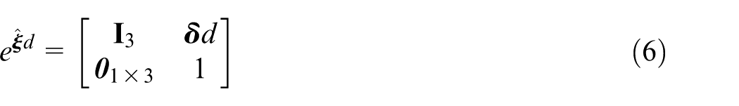
On the basis of the twist coordinates of variations, the fluctuation of key characteristic point (KCP) on the component variable from its nominal position to its real position caused by one manufacturing variation can be mathematically described by
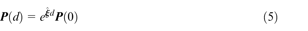
where
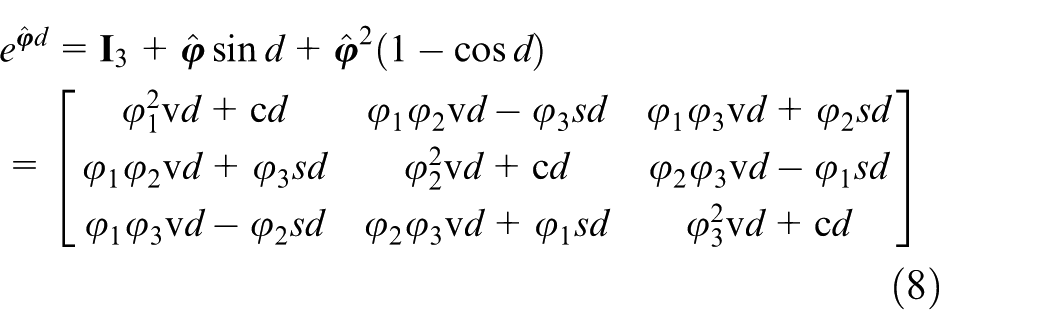
where
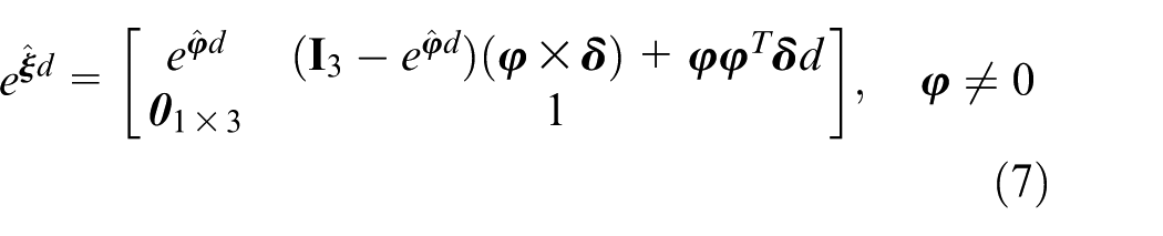
where
Up to now, we have presented the mathematical description of the fluctuation of KCP caused by one individual variation using the exponential map. In order to derive the complete description of variation propagation in the assembly, we first mark the component variables sequentially around the assembly vector loop, and the total number of individual variations is n. Assume that all the individual variations are zero except the last one. Then, the assembly variations will be the functions of the nth individual variation only, that is,
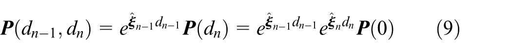
By the same token, when all the individual variations are taken into account, the variation propagation can be described by the POE as
where

Here,
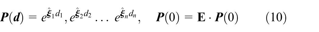
Based on the explicit stack-up functions, the worst-case (WC) and statistical variations can be analyzed. Let all the individual variations meet their extreme tolerance values. Substituting these values into the stack-up functions will produce 2 n results for each assembly variation. The maximum and minimum values are just the WC assembly variations. However, to each individual variation a probability distribution is assigned, usually the normal distribution. Then, the statistical distributions of assembly variations can be obtained using the Monte Carlo simulation. The assembly variation range is assumed as ±3σ, where σ is the standard deviation. 1 The main processes of tolerance analysis based on the POE formula are summarized in Figure 2.
Main processes of tolerance analysis via the POE formula.
Case study
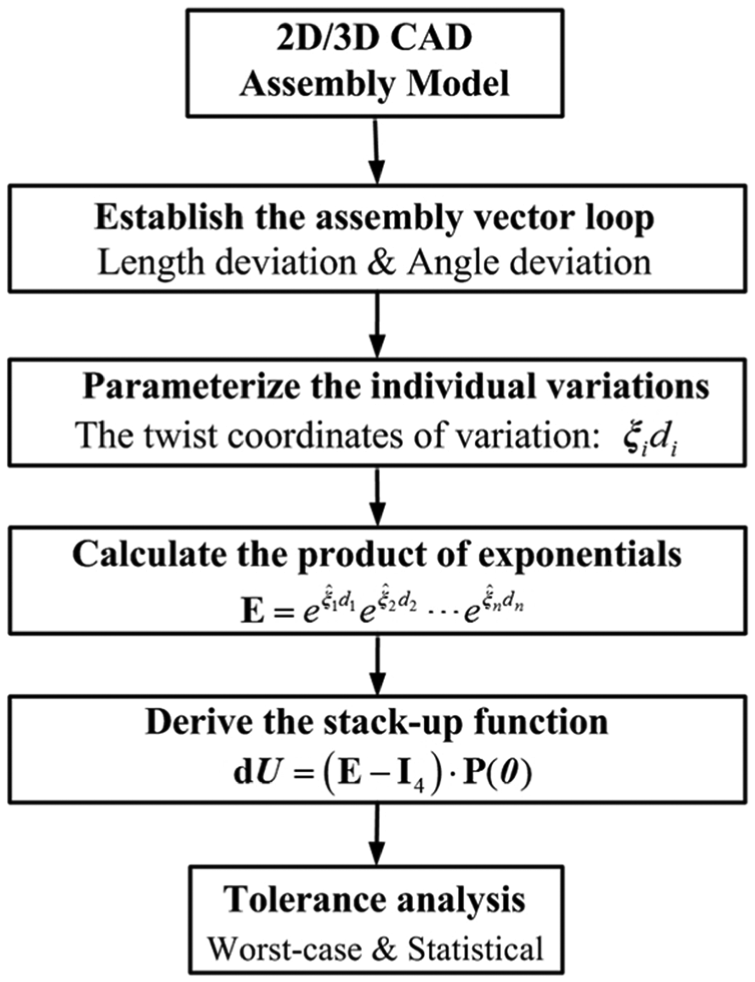
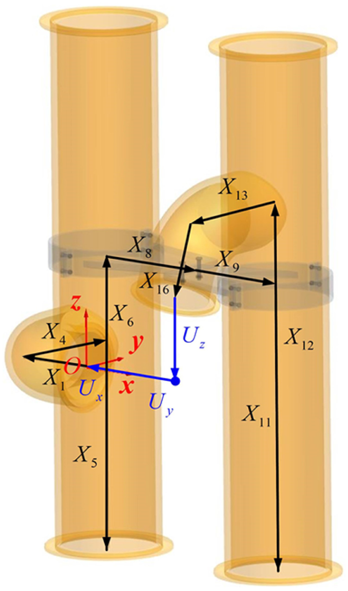
In this section, a pipeline assembly case consisting of two straight main pipes is studied. Each main pipe extends an elbow. The communicating pipe is finally installed in order to connect the end flanges of elbows. Because of the existence of manufacturing variations, the relative positions between the two end flanges are inevitably fluctuant, which may further cause the failure of assembly. In consequence, it is necessary to perform the tolerance analysis in order to control the relative positions of the two end flanges. The CAD model is exhibited in Figure 3, and Figure 4 shows the basic dimensions of the assembly.
CAD model of the assembly case.
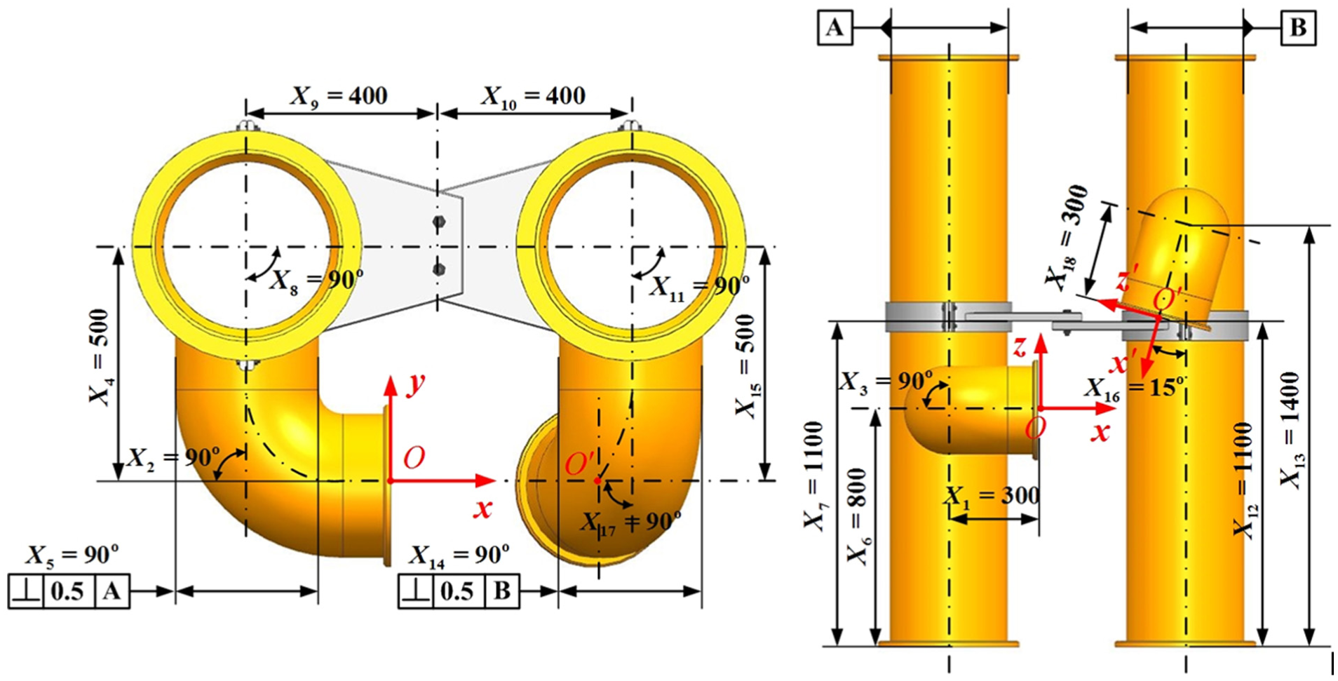
Basic dimensions of the assembly case.
According to Figure 4, there are 18 variation sources in this assembly, and two of them are perpendicularity tolerances. Figure 5 shows an equivalent of the perpendicularity in this case.
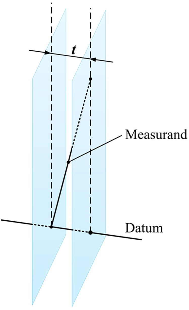
Equivalent of the perpendicularity tolerance.
Design tolerances of the assembly case.
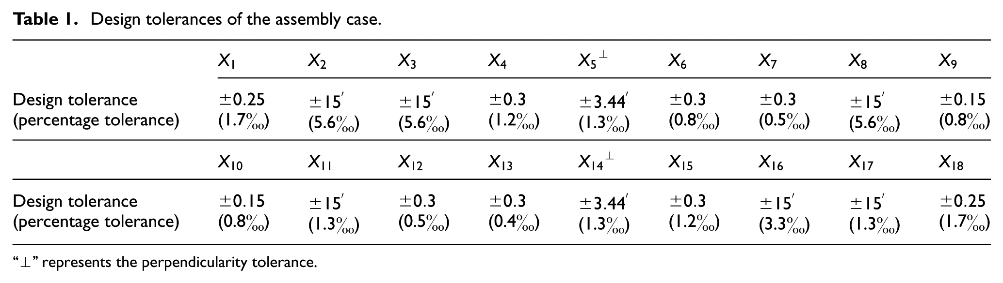
“⊥” represents the perpendicularity tolerance.
Tolerance estimation using different approaches
The exact geometric solutions
For the convenience of verifying the feasibility of the POE formula in tolerance analysis, the exact values of assembly variations are analyzed at first. Let the global DRF be located at the center of the end flange1, as shown in Figure 4. Then, the relative positions of the two end flanges can be determined by three assembly variables indicated by Ux, Uy and Uz. According to the geometric assembly relations of the pipeline assembly case, the analytic expressions of assembly variables associated with the component variables can be easily derived. Seeing that there are up to 18 component variables in this case, the concrete expressions of the assembly variables are very sophisticated and are not given at here. It can be derived that the nominal values of the assembly variables as
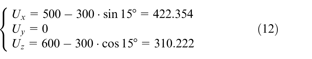
Furthermore, calculating the extreme solutions of the assembly variables, the differences between the extreme solutions and the nominal values are just the exact WC assembly variations, that is
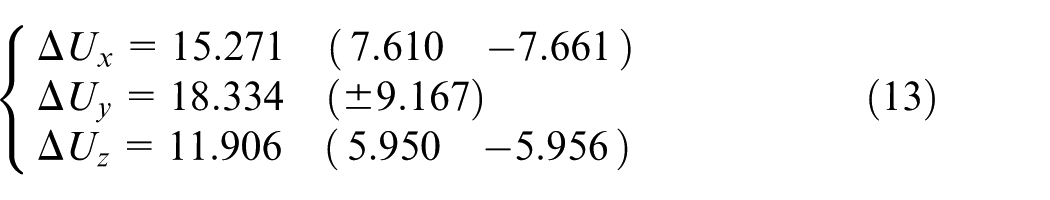
The parentheses () indicate the upper- and lower-limit deviations of the relative positions.
POE formula
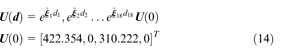
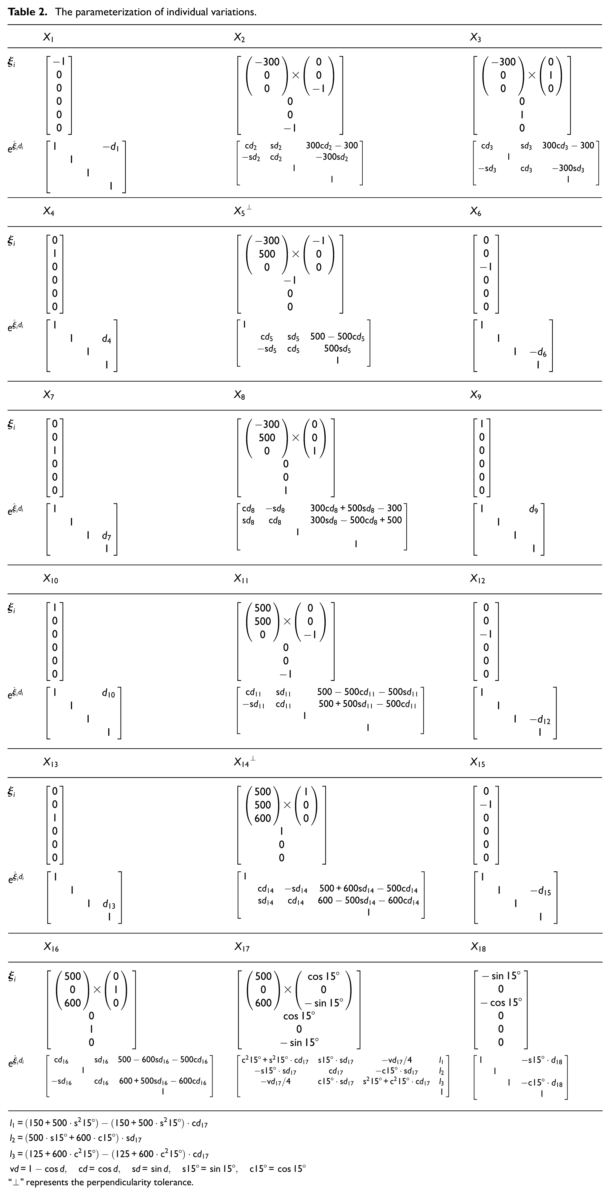
Next, the pipeline assembly case is studied via the POE formula. Also, choose the center of the end flange1 as the origin of global DRF. By analyzing the structure of the assembly, the vector loop is drawn, as shown in Figure 6. Combing with the CAD model, it is not hard to get the twists of the individual variations. The corresponding exponential maps can also be obtained according to formula (6) and (7). Table 2 lists the twists and exponential maps of the 18 contributors. The tolerance accumulation can be expressed as
Assembly vector loop of the POE tolerance analysis.
The parameterization of individual variations.
“⊥” represents the perpendicularity tolerance.
where
Based on formula (14), three analytic and nonlinear stack-up functions are derived. The functions can directly relate the variations of relative positions to the individual variations. Since the stack-up functions are very sophisticated with 18 independent variables, it is not convenient to present the complete forms here. However, once indicated with

Then, the WC and statistical variations in the relative positions can be calculated. The tolerance analysis results are shown in Table 4 with comparison to the exact geometric solutions.
DLM
As a contrast, the DLM that is a common 3D tolerance analysis model is used to estimate the variations in relative positions between the two end flanges caused by the 18 contributors. Like the POE formula, the DLM also needs to build the assembly vector loop. Nevertheless, the stack-up functions derived by the DLM are linear, and the sensitivity matrix is used to map the individual variations to the assembly variations.
Figure 7 presents the assembly vector loop of the DLM. In order to describe the variation propagation around the vector loop, the local DRF is established for each vector. Then, the tolerance accumulation is described by a concatenation of homogeneous transformation matrices. The frame
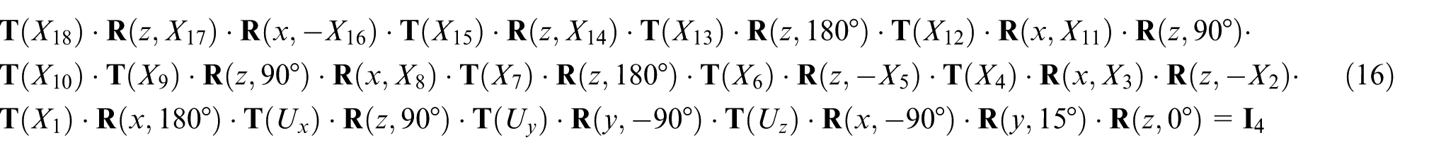
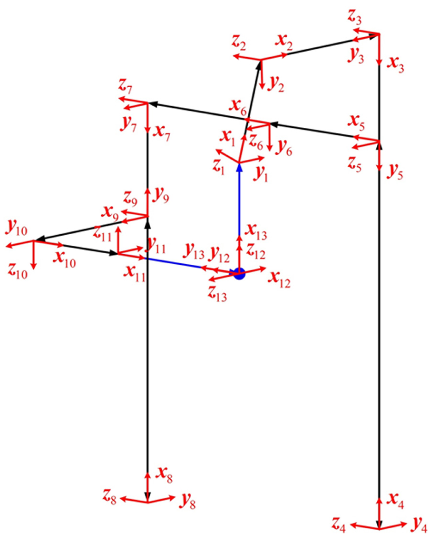
Assembly vector loop and local DRFs of the DLM.
where
Based on the first-order Taylor’s series expansion on formula (16), the assembly sensitivity matrix
Assembly sensitivity matrix derived by the DLM.
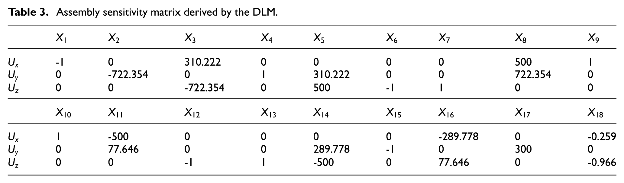
Combining with the design tolerances of the contributors, the WC and statistical variations can be, respectively, calculated according to the WC and root sum square (RSS) methods.3,6 The analysis results are also shown in Table 4.
Tolerance analysis results of different methods.
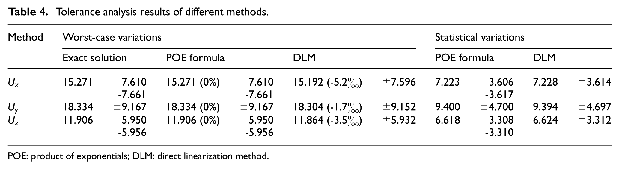
POE: product of exponentials; DLM: direct linearization method.
Result comparison and analysis
From Table 4, the worst-case variations obtained by the POE formula are consistent with the exact solutions; whereas, there are some differences between the worst-case variations in the DLM and the exact solutions. The differences are quantified in percentage in Table 4. It is clear that the POE formula can lead to a higher accuracy in tolerance analysis than the DLM. As we have known, the DLM extracts the constraints of variations based on the linearization of the analytic assembly response function. The linear stack-up function (formula (17)) neglects the high-order variations which represent the couplings of variation sources. In result, the truncation errors are produced. 24 In contrast, the stack-up functions derived by the POE formula are nonlinear and can directly relate the assembly variations to the individual variations. Therefore, the truncation errors are eliminated in the POE tolerance analysis.
In addition, it can be seen that the assembly variations in both the exact solutions and the POE formula are asymmetric even though all the component tolerances are symmetric. Meanwhile, the values of upper- and lower-limit deviations of Ux, Uy and Uz obtained by the DLM are all equal. This phenomenon can be well interpreted using a simple example shown in Figure 8, in which the assembly constraint function can be described by a nonlinear equation of
An example of nonlinear variation source.
In fact, the errors in tolerance analysis caused by the linear stack-up function are generally acceptable. In the pipeline assembly case, the precision of tolerance analysis via the POE formula is increased by 0.52% at the most compared with that of the DLM. In consideration that the design tolerances of the component variables are all very small, and some of which even less than 0.1% of their nominal dimensions (Table 1), the truncation errors arising from the linearization are indeed small. However, if the individual variations in the nonlinear contributors are increased, or if the assembly problem is seriously nonlinear, the improvement in precision of tolerance estimation using the POE formula rather than the existing linear tolerancing models will be significant.
In addition, comparing formulae (14) and (16), it is clear that the variation propagation described by the POE formula is more concise. Moreover, the POE formula performs the tolerance analysis with only one global DRF, while many existing models including the DLM need to build local DRF for every feature in the assembly. Therefore, the tolerance analysis processes via the POE formula are more simple and convenient. Also note that the POE formula is a zero reference position description. That is to say, the twist coordinates of individual variations are all obtained in the nominal state of the assembly. If a standard CAD model is provided, it is convenient to parameterize all the individual variations in turn by the computer. Finally, the computer-aided tolerancing is possible to be developed.
Conclusion
In this article, a new method termed as the POE formula is introduced to perform the tolerance analysis of mechanical assemblies. The method describes the component variations and tolerance accumulation using the twist coordinates and the POE, respectively. Consequently, the nonlinear stack-up functions relating the assembly variations to the individual variations are derived, by which the worst-case and statistical assembly variations can be calculated.
In order to verify the feasibility and advantages of the proposed method, a 3D pipeline assembly case is studied with comparison to the exact geometric solutions and the DLM. Under the circumstances that the individual variations are all very small compared with their nominal dimensions, the POE formula leads to an increase of 0.52% at the most in precision of tolerance analysis than the DLM. Besides, the estimation of limit deviations exploiting the proposed method is also more accurate. Due to the elimination of local DRFs, the description of variation propagation via the POE formula is laconic and convenient. The zero reference position description further makes it possible to integrate the method with commercial CAD system to develop the computer-aided tolerancing.
Footnotes
Declaration of conflicting interests
The author(s) declared no potential conflicts of interest with respect to the research, authorship and/or publication of this article.
Funding
The author(s) disclosed receipt of the following financial support for the research, authorship, and/or publication of this article: This work was supported by the National Basic Research Program of China (grant no. 2014CB046600), the National Science and Technology Major Project (grant no. 2014ZX04001-081-08) and the SJTU SMC-Morningstar Young Scholars Program (grant no. AF0200105).