
Abstract
The performance of mechanical products is closely related to their key feature errors. It is essential to predict the final assembly variation by assembly variation analysis to ensure product performance. Rigid–flexible hybrid construction is a common type of mechanical product. Existing methods of variation analysis in which rigid and flexible parts are calculated separately are difficult to meet the requirements of these complicated mechanical products. Another methodology is a result of linear superposition with rigid and flexible errors, which cannot reveal the quantitative relationship between product assembly variation and part manufacturing error. Therefore, a kind of complicated products’ assembly variation analysis method based on rigid–flexible vector loop is proposed in this article. First, shapes of part surfaces and sidelines are estimated according to different tolerance types. Probability density distributions of discrete feature points on the surface are calculated based on the tolerance field size with statistical methods. Second, flexible parts surface is discretized into a set of multi-segment vectors to build vector-loop model. Each vector can be orthogonally decomposed into the components representing position information and error size. Combining the multi-segment vector set of flexible part with traditional rigid part vector, a uniform vector-loop model is constructed to represent rigid and flexible complicated products. Probability density distributions of discrete feature points on part surface are regarded as inputs to calculate assembly variation values of products’ key features. Compared with the existing methods, this method applies to the assembly variation prediction of complicated products that consist of both rigid and flexible parts. Impact of each rigid and flexible part’s manufacturing error on product assembly variation can be determined, and it provides the foundation of parts tolerance optimization design. Finally, an assembly example of phased array antenna verifies effectiveness of the proposed method in this article.
Keywords
Introduction
In the assembly process of mechanical products, product surface features associated with performance always deviate from their ideal positions due to manufacturing error of parts. It leads to the reduction of product performance, and products may even be discarded when assembly variation exceeds a certain level. Therefore, product assembly variation’s prediction and control is a hot issue that engineers concern about. Mechanical parts are divided into two categories, rigid parts and flexible parts, based on their stiffness. The rigidity of rigid parts is high and its anti-deformation ability is strong. Only linear transfer of parts’ manufacturing errors is considered in variation analysis, while their deformations are ignored in the assembly process. Methods of tolerance chain or small displacement torsor (SDT) are applied to solve rigid parts’ assembly problem. Transfer matrix is always used to calculate the cumulative error of product surface through coordinate transformation. And assembly variation is represented by product spatial position and posture compared to its nominal state in multiple degrees of freedom. Contrary to rigid parts, flexible parts have a low rigidity and they are easy to deform. 1 Deformations must be considered in their elastic regions during assembly process. Due to the nonlinear relationship of constraint equations, finite element method is often used to acquire the assembly variation. In this way, flexible parts’ surfaces are partitioned to discrete feature points to calculate the deformations after assembly through elastic mechanics equations. Aircraft skin-stringer structure is taken as an example of typical complicated mechanical products. It consists of rigid parts (stringers, wallboards, frames, etc.) and flexible parts (skins). Neither rigid variation analysis nor flexible variation analysis can apply to this sort of complicated products. And the existing researches on rigid–flexible hybrid models are superficial, which is difficult to obtain the quantitative relationship between product assembly variation and manufacturing errors of each rigid and flexible part. Therefore, a uniform assembly variation model is demanded to predict complicated product assembly variation for rigid–flexible tolerance optimization. 2
The existing research on rigid body assembly variation is relatively mature, and a variety of rigid body assembly variation analysis methods including two-dimensional tolerance chain model and three-dimensional (3D) SDT model have been developed. Hu et al. 3 constructed a model describing the variation in the dimensional chain of stroke-related mechanical assemblies. The results showed that the variation in the dimensional chain induced by working conditions could not be ignored in the tolerance design stage. Jin and Shi 4 defined tooling locating error, part accumulative error and re-orientation error, and proposed a state-space modeling approach to characterize the inherent relationships among them for dimensional control of rigid assembly processes. Ding et al. 5 used a two-dimensional state-space model to calculate the variation in the multi-station assembly process. Following the sensitivity analysis in control theory, a group of hierarchical sensitivity indices is defined and expressed in terms of system matrices to discuss variation control. Huang6,7 extended rigid variation model to 3D space and built the 3D rigid assembly model under both single-station and multi-station processes. Method of stream-of-variation analysis (SOVA) is proposed and it is adaptive for more complex assembly process of rigid products. Asante 8 established a relationship between the tolerance zone of features and torsor parameters according to the constraints specified for features. And workpiece geometric error, locator geometric error, clamping error were accumulated in workpiece fixturing process. Liu et al. 9 established a more general state-space model by adopting differential motion vector (DMV) method. Deviations with respect to four types of coordinate systems (global, fixture, part, feature coordinate system) were modeled and a series of homogeneous transformation matrices were formulated to calculate assembly variation induced by part fabrication processes.
In the early research phase of flexible assembly variation model, researches always used Monte Carlo method to calculate each assembly variation corresponding to parts’ manufacturing errors in a certain tolerance interval. This method needed a large number of data sampled from flexible parts surfaces, and its computation efficiency was very low as the amount of data increased. Liu and Hu 10 proposed the method of influence coefficients (MIC), which reduced the number of finite element analysis (FEA) greatly compared to Monte Carlo method. By constructing the sensitivity matrix of all nodes on the thin-plate structure, they established a linear relationship between assembly deviation and parts’ initial manufacturing errors. Many flexible assembly variation methods proposed afterward were a kind of application and expansion based on MIC. Camelio et al. 11 found that fluctuation of points on flexible part surface had an influence on neighboring points. Deformations on nodes depended on the geometric relationships among these discrete points and the stiffness of flexible part. A covariance matrix was used to describe the relationships of neighboring points on the same surface to calculate the final deviations. According to feature functions, Yu and Yang 12 divided the surface features into four types: basic locating points, additional locating points, measurement points and welding points. A linear relationship between the input part variations and the output assembly variation was established by flexible variation analysis. Tonks and Chase 13 proposed an orthogonal polynomial-based covariance model to account for surface variations of the compliant parts over a wide range of wavelengths. A series of Legendre polynomials were used to approximate the actual geometric shape of the plane to model the surface features of parts. Huang and Ceglarek 14 used a discrete cosine transform (DCT) to model flexible part form errors. He decomposed the error fields into a series of independent error modes to represent different kinds of errors in manufacturing processes. The relationship between tolerance expression and uncertainty factors was established. Liao and Wang 15 proposed a new method based on wavelet analysis and the finite element method for variation analysis of flexible assemblies. The final assembly deviations were predicted according to part variations in different scales. Zhang et al. 16 proposed two methods of modeling geometric form errors for single parts based on linear combination of basis shapes and modeling statistic geometric form errors for a batch of parts machined on the basis of principal component analysis.
When solving practical engineering problems, part deformations due to force and other nonlinear factors make flexible assembly analysis more complex. Mei et al. 17 constructed an assembly variation model based on the elasticity mechanics and interval approach for compliant aeronautical structures. It was suited for linear and linearized nonlinear assembly systems. Wang et al. 18 proposed an assembly deformation prediction model and a variation propagation model to predict the assembly variation of aircraft panels. Equations of statics of elastic beam are used to calculate the elastic deformation of panel component while considering the nonlinear behavior of physical expressions. Guo et al. 19 developed a low-cost flexible assembly tooling system for different wing components. Two kinds of positioning method and the corresponding assembly precision were studied to improve the assembly accuracy of aircraft wing components. Liu et al. 20 developed a physical simulation method of product assembly and operation manipulation based on statistically learned contact force prediction model. Contact force and deformations were acquired based on hidden Markov model and local weighting learning in real time. Zhang et al. 21 proposed a quantitative variation propagation modeling method, highlighting the subsequent impact of initial residual stress on raw material. Legendre polynomials and spline functions were employed for modeling variation propagation in a case study of the horizontal stabilizer assembly system.
Some scholars showed interest in the assembly process of rigid–flexible hybrid products. They predicted the final assembly variation of these complicated mechanical products by combining existing methods of variation analysis. Franciosa 22 used SVA-TOL (statistical variation analysis for tolerancing) and SVA-FEA (statistical variation analysis and finite element analysis) methods to analyze the assembly variation of rigid and flexible parts separately. The former constructed tolerance expression according to ISO standard. Rigid parts’ assembly variation model was established by features of points, lines and surfaces, and the least square method was used to solve equations. The latter introduced a global sensitivity matrix to correlate inputs (parts manufacturing errors or process variation) and outputs (assembly variation), which avoided the huge computational complexity of Monte Carlo method. Ghandi and Masehian 23 proposed the concept of assembly stress matrix (ASM) to describe interference relations between parts of an assembly and the amount of compressive stress needed for assembling flexible parts. The Scatter Search optimization algorithm was customized for this problem to find the optimal assembly sequence of rigid–flexible hybrid products by a TOPSIS-Taguchi-based tuning method. Ni et al. 24 constructed the finite element models for fixtures and parts. Their nodes were ordered according to an appointed assembly sequence. Three noncollinear feature points were selected and their translational displacements (gaps) were calculated by kinematic formulations representing the part rigid motion. Compliant motions were reached by the modified FE analysis using the gap-induced rigid motions and deformations. Cai et al. 25 applied DMV and MIC to obtain rigid variation in the in-plane direction and compliant variation in the out-of-plane direction. Three types of variation sources that were fixture locators’ deviations, datum features’ deviations and joint features’ deviations were considered to predict assembly variation. These methods are just a simple superposition of rigid and flexible part errors. They fail to realize the uniform variation model of rigid–flexible hybrid system and cannot determine numerical relationship between final product assembly variation and rigid/flexible part errors. It is difficult to serve the optimal design of tolerances for product quality.
In order to solve the inadequacies of existing methods mentioned above, a kind of complicated products’ assembly variation analysis method based on rigid–flexible vector loop is proposed in this article. Variation analysis model is improved considering variations of flexible parts, based on traditional vector loop which is only applied for rigid parts. Unlike the vector representation of rigid part, flexible part variation cannot be modeled by a single vector. A discrete method which discretizes flexible part into a set of multi-segment vectors is applied. And each vector is orthogonally decomposed into two components. One is along the direction of flexible part’s ideal sideline, representing position information of discrete feature points on the flexible part surface. The other one is along the vertical direction of flexible part’s ideal sideline, describing each discrete feature point’s error magnitude. Combining the multi-segment vector set of flexible part with traditional rigid part vector, a uniform vector-loop model is built to represent variations of rigid–flexible hybrid complicated products. Shapes of part surfaces and sidelines are estimated according to different tolerance types, and probability density distributions of surface discrete points are calculated in statistical method based on surface analytic expression. Means and variances of these discrete points are different according to tolerance type and tolerance field size of the flexible part. They are substituted into flexible multi-segment vector model, and direct linearization method (DLM) is applied to calculate statistic errors based on rigid–flexible vector-loop model.
Compared with the existing methods, relationship between the key feature errors of products and the manufacturing errors of all parts is acquired, so as to predict the final assembly variation of rigid–flexible hybrid complicated products. The proposed method is helpful to optimize product tolerance design. Comparison between existing methods and proposed method is shown in Figure 1.
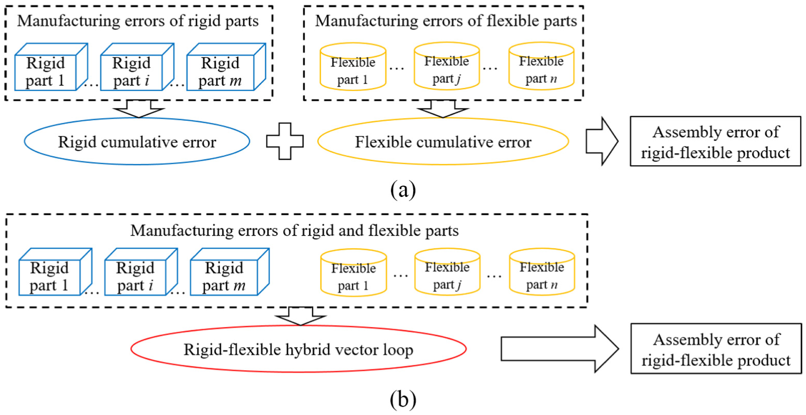
Comparison between (a) existing methods and (b) proposed method.
Discrete statistical expression of part surface error characteristics
According to the different forms of expression, manufacturing tolerances of parts can be divided into three categories: size tolerance, position tolerance and shape tolerance. Among them, position tolerance includes parallelism, perpendicularity, angularity, concentricity, symmetry, position, circle runout and total runout. Shape tolerance is composed of straightness, flatness, circularity, cylindricity, line profile and surface profile. Assembly manner of mechanical product is mostly surface fit, and only error transfer in the normal direction of surface is considered generally. 26 Figure 2(a) is shape error of a cuboid part. Only the variation of part upper surface z = 0 is considered, and its direction is along the y-axis. The red dashed line indicates the upper and lower boundaries of part shape tolerance, and the black solid line indicates the actual position of part upper surface with a certain error. When the feature has a similar shape along z-axis, this surface error can be simplified the characterization of part sideline as Figure 2(b). Different types of manufacturing errors tend to have similar performance, and part error composition cannot be determined according to a specific surface shape. Therefore, one type of tolerance is considered for a single feature in the research acquiescently. In Figure 2, only shape error of cuboid part is analyzed, regardless of its size and position error, so as to avoid confusion.
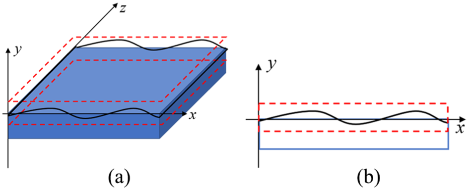
Simplified characterization of (a) part surface error to (b) part sideline error.
The part sideline can be characterized by an infinite number of discrete points as continuous feature. Distance between the actual position and the ideal position of each discrete point constitutes the specific shape of sideline according to tolerance type. As shown in Figure 3, all the discrete points on the sideline with dimensional error have the same deviation value. So a single vector can be used to characterize size tolerance, which is generally applicable to the rigid body error propagation model such as tolerance chain. For sidelines with position tolerance and shape tolerance, a finite number of discrete points are chosen to simulate them approximately, and manufacturing errors are represented by a set of vectors.
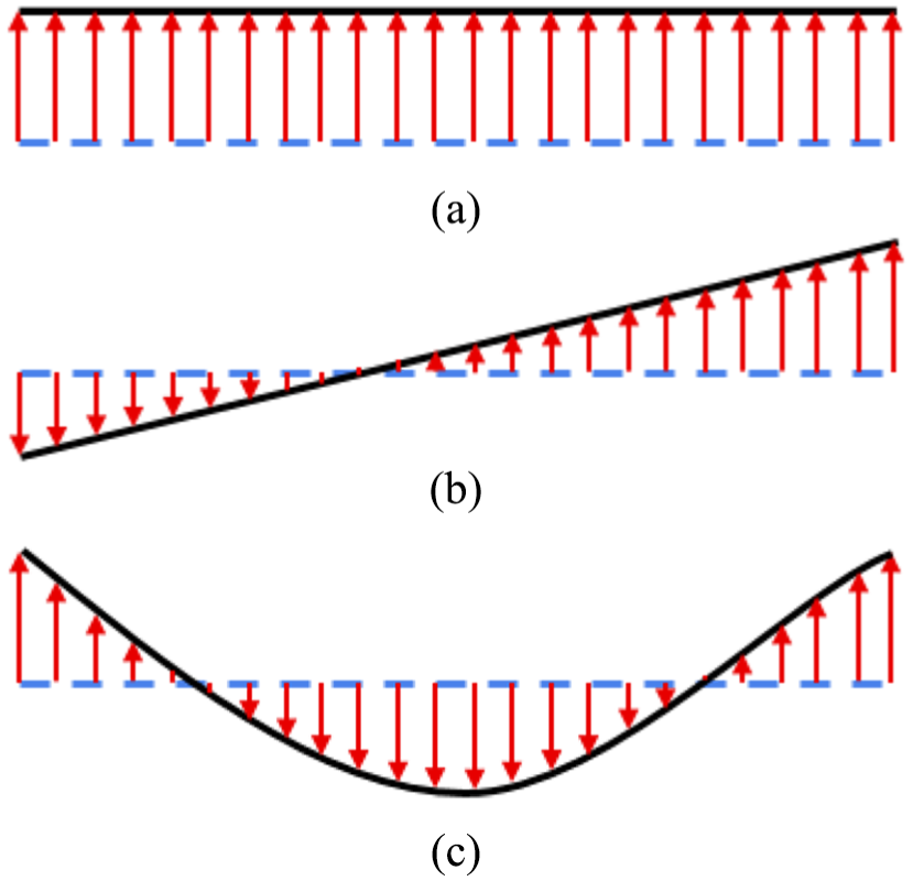
Different types of sideline errors: (a) dimension error, (b) position error and (c) shape error.
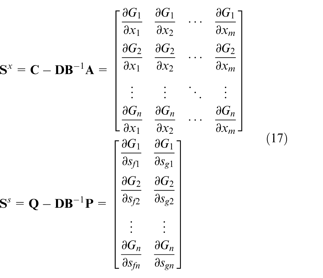
During the statistical variation analysis process, most scholars treat sidelines with position tolerance and shape tolerance as that with size tolerance. All the discrete points on a sideline are considered that they are independent of each other and have the same mean and variance. However, there is an association between discrete points on a part sideline because of surface continuity. They will have different statistical distributions according to their positions with a specific error shape. In this section, parallelism and flatness of parts are taken as an example, to determine the statistical distributions of all discrete points on sidelines with these two kinds of errors based on their analytic expressions.
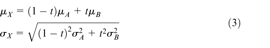
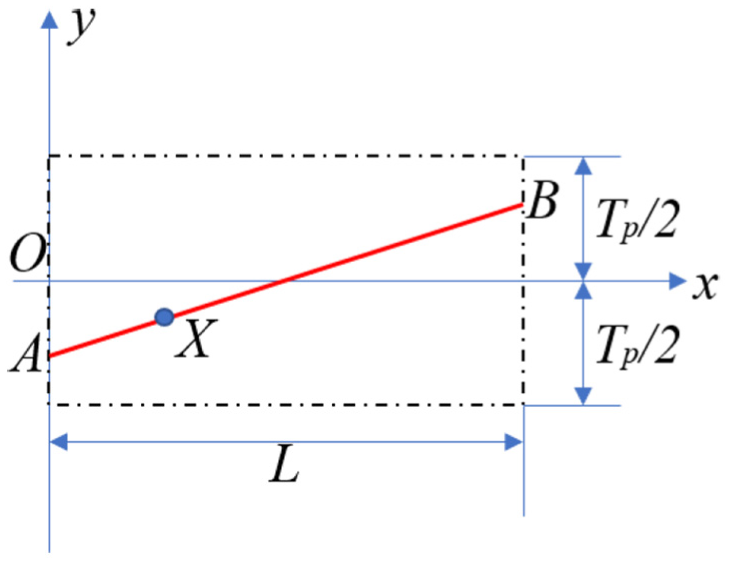
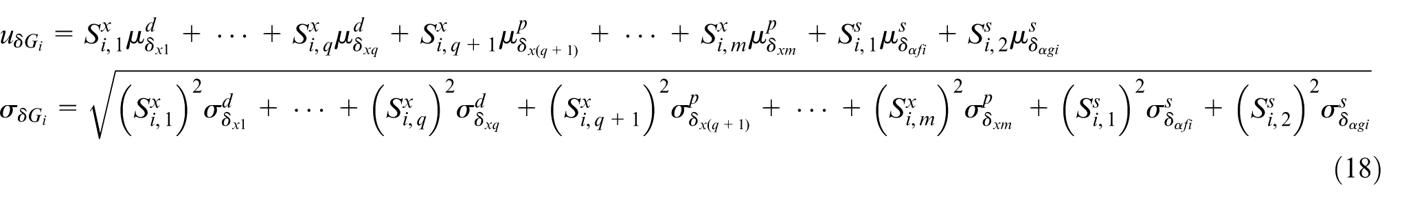
The planar structure’s sideline is illustrated whose ideal state is a horizontal straight-line segment with two endpoints A and B. Two-dimensional coordinate system is constructed such that x-axis coincides with segment AB, and y-axis is perpendicular to segment AB while passing through endpoint A. L is the length of segment AB, so
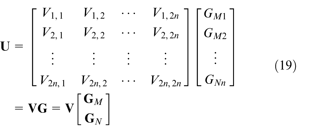
1. Discrete representation of part sideline with parallelism
Part parallelism tolerance is expressed as Tp. In the x–y coordinate system, part sideline’s shape description with parallelism appears as a linear function which has an angle with x-axis, as shown in Figure 4. The expression of parallelism is

Two-dimensional description of part parallelism.
Generally, the upper and lower deviations are set as +Tp/2 and −Tp/2, and y value of any point X satisfies
2. Discrete representation of part sideline with flatness
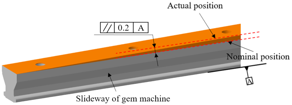
Parallelism error of gem machine slideway.
Statistical expression of gem machine slideway parallelism error: (a) standard deviations of points and (b) 1000 sampling cases in parallelism zone.
Part flatness tolerance is expressed as Ts. In the x–y coordinate system, description of part sideline’s deviation appears as a quadratic function in most situation, as shown in Figure 7. The expression of flatness is
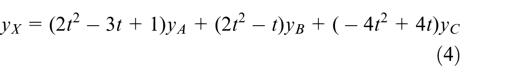
Two-dimensional description of part flatness.
The upper and lower deviations of flatness are set as +Ts/2 and −Ts/2. Here, A, B and C are initial points and they obey the equation
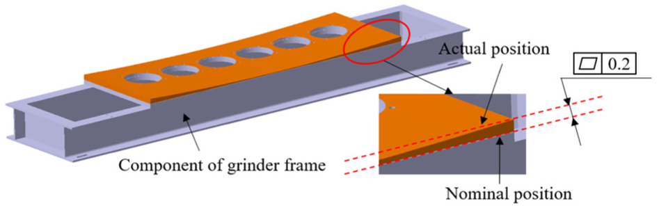
Flatness error of grinder frame component.
Statistical expression of grinder frame component flatness error: (a) standard deviations of points and (b) 1000 sampling cases in flatness zone.
Through equations (2)-(5), mean values and variances of all discrete points on parts with parallelism and flatness tolerance can be calculated. When part’s tolerance field is symmetrically distributed with respect to the ideal position, as well as the selected points have the same normal distribution, mean values of all discrete points on the sideline are zero. However, their variances in y-axis are different with each other. They should be calculated by equations (3) or (5) according to tolerance type, instead of assuming that each discrete point has the same variance.
Construction of rigid–flexible hybrid vector-loop model
Traditional vector-loop model only aims at size and position deviations of rigid parts. The cumulative error of product target feature is obtained by calculating the linear transmission relation between parts during the assembly process. Based on this method, a kind of rigid–flexible hybrid vector-loop model is proposed in this section, which considers shape errors of flexible parts at the same time. A simple assembly example of five parts is shown in Figure 10. There are assembly relationships among part 1, part 2 and part 3. Part 2 and part 3 are, respectively, assembled with part 4 and part 5. Vector-loop model will be constructed based on this assembly example to predict the cumulative assembly variation, which is reflected as the gap between part 4 and part 5.
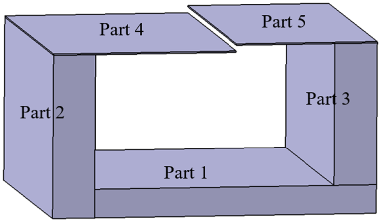
A simple assembly example of five parts.
Transfer model of rigid assembly variation
According to the theory of SDT, features’ slight changes in one or several degrees of freedom are applied to represent dimensional and angular deviations of rigid parts. Translation vectors and rotation vectors are constructed to express the deviations of its actual and ideal states. For ease of calculation, these vectors are transformed into a series of 4 × 4 homogeneous matrices based on kinematics of robotic motion.
As shown in equation (6),
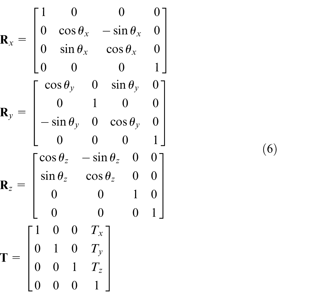
When multiple rigid parts with size and position deviations are assembled, the final accumulated error can be obtained by multiplying each part’s transformation matrix in accordance with assembly relationship. 27 It can be expressed in the following form as in equation (7)

where
Assuming that parts in Figure 10 are all rigid, a rigid vector model in 3D space is constructed as shown in Figure 11(a). Figure 11(b) is a simplification of Figure 11(a) which neglects thickness of parts 1–3. It is known from these two images that it is confusing to consider all vectors in different directions. A closed loop is hard to be formed for describing variation propagation during assembly process. Besides, the target vector is often not referred to vectors of all three directions. For example, gap in Figure 11 which is represented by vector G has no concern with vectors along z axis. Therefore, one or more two-dimensional vector loops are usually modeled to deal with 3D assembly problems in accordance with requirements.
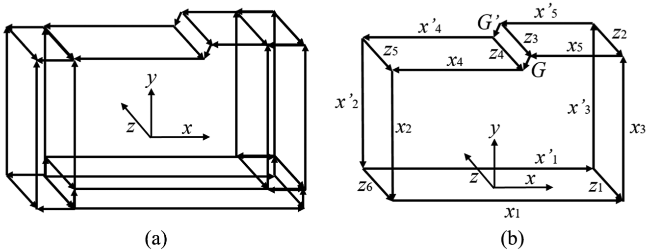
Rigid vector model in 3D space: (a) considering thickness of parts 1–3 and (b) neglecting thickness of parts 1–3.
A two-dimensional rigid vector-loop model is constructed in x–y plane as shown in Figure 12.
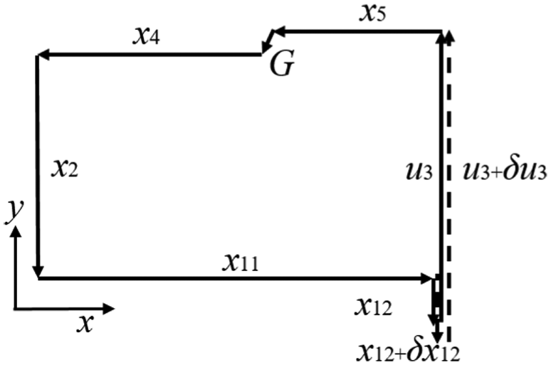
2D rigid vector-loop model in x–y plane with variables
For small variations of parts in their tolerance zones, the first-order Taylor expansion is applied and equation (7) can be approximated by DLM as in equation (8). Equations of multiple rigid assembly vector-loop model are required in global coordinate system, in which
Converting equation (8) to a matrix form as following, where
For a closed-loop structure, the set of assembly variables

If
For the open-loop structure, the partial differential matrices of

Rigid–flexible hybrid assembly variation model
Thin-walled metal sheet is a kind of representative flexible part which is widely used in industry. Deformation in the direction perpendicular to the plate is much larger than that in other directions. Therefore, when making a variation analysis of flexible thin-walled plate with shape error, only cumulative error in the direction perpendicular to the plate should be considered. As mentioned in section “Discrete statistical expression of part surface error characteristics,” shape errors of flexible parts are simplified to errors of their sidelines in this section. Sidelines of flexible parts with shape errors cannot be represented by single vectors due to their uneven appearances. Generally, a sideline is divided into many discrete points and a set of multi-segment vectors is applied to express the sideline. And this set of vectors representing flexible part can be combined with rigid part vector-loop model in equation (10).
Assuming part 4 and part 5 in Figure 10 are two flexible thin-walled structures instead of rigid parts, it can be considered as a simple rigid–flexible assembly model. The flexible vectors of these two flexible thin-walled structures with shape errors are illustrated by partial description as shown in Figure 13. The sidelines are both divided into n discrete feature points and they exist a relationship of one-to-one correspondence to be assembled. Gaps between them are recorded as a set {G}. In order to calculate the variations of gaps between all pairs of corresponding feature points, n vector-loop models need to be constructed. Variable vectors fMj and fNj are 3D vectors of flexible parts M and N. They are connections of the jth discrete point with starting point of sideline to represent feature points’ states. It is noteworthy that the direction of fMj is toward each feature point from starting point, but the direction of fNj is toward starting point from each feature point. Adding these errors into traditional rigid part vector-loop model in section “Transfer model of rigid assembly variation,” and corresponding partial differential matrix is defined as

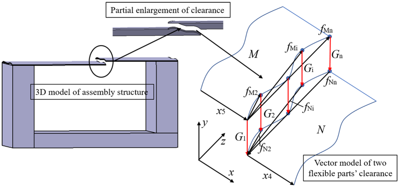
Assembly of two flexible thin-walled structures with shape errors.
However, when the number n of discrete feature points is too large, computational efficiency is very low that describes shape errors of flexible parts by variable vector f. Then variable vector f is decomposed into two components as shown in Figure 14. One component is recorded as r representing position of feature point, whose direction is along the ideal sideline of flexible part and is consistent with z-axis of the global coordinate system. Its size equals to the spacing between projection of feature point on ideal sideline and starting point. If the sideline length of flexible part is L, the ith feature point has a distance ti × L with starting point along z-axis, where ti is a series of numbers in interval [0, 1]. Another component is defined as s representing deviation in a certain shape tolerance Ts, whose direction is perpendicular to the ideal sideline of flexible part and is consistent with y-axis of the global coordinate system. Its size can be calculated according to the probability density of discrete feature points on sidelines under different tolerance types in section “Discrete statistical expression of part surface error characteristics.”
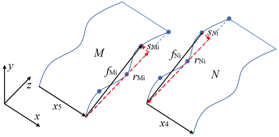
Decomposition of variable vector f into two components.
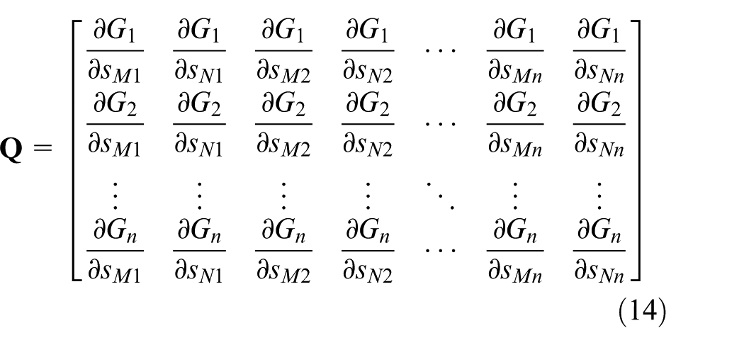
Since only variations of two flexible parts in the y-axis are considered, the partial derivative of assembly variables {G} with respect to component r which is along z-axis is 0. The shape error set of flexible parts
Combined with equation (12), the assembly variation model of rigid–flexible hybrid complicated product can be obtained by equation (15). The structure is open-loop and it is a statically determinate system. Matrix
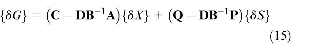
Equation (15) is the general form of a rigid–flexible hybrid vector-loop model.
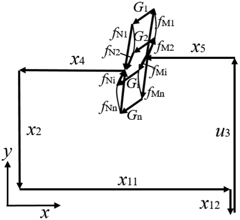
Diagram of rigid–flexible hybrid vector-loop model.
Deformation prediction of rigid–flexible hybrid assembly
A rigid–flexible hybrid assembly vector-loop model is constructed in section “Construction of rigid–flexible hybrid vector-loop model.” The coefficient matrices of rigid part errors and flexible part errors in equation (15) are, respectively, defined as

Expressions of
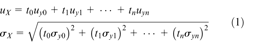
Due to discretization of flexible part sideline into several feature points based on the rigid–flexible vector-loop model, probability density distributions of all points need to be determined, respectively, according to their positions through the method in section “Discrete statistical expression of part surface error characteristics.” Then means and variances of product measured features can be calculated as shown in equation (18)
Statistical distributions of {GM} and {GN} are obtained which describe gaps of parts M and N with their ideal positions, respectively, and they are used for assembly variation analysis as input through MIC to acquire final assembly deformation. Suppose sidelines of two flexible parts both have n discrete feature points and these points will be assembled together. Their nominal positions are identical so the assembling points follow a one-to-one correspondence. After assembly, these points are defined as measure points of product to predict assembly quality. As part stiffness matrix is determined by its material, structure and other factors, it is difficult to be obtained by analytical method. MIC is utilized to calculate the stiffness matrix approximatively and distributions of measure points are gained to complete deformation prediction.
According to the rigid–flexible hybrid vector-loop model, initial errors
Step 1. A unit force whose direction is the same as the direction of initial error is applied to the jth (j=1, 2, …, 2n) source of variation. The first FEA is used to calculate the response of all measure points. The displacements of nodes are recorded in a column vector
Step 2. Based on the elastic mechanics equations about stress and stiffness of parts, relationship of matrices
Step 3 Reaction forces through step 2 are applied to each feature point. Then the second FEA is used to calculate the spring-back displacements at key points in the y-axis direction for the welded structure. Vij (i = 1, 2, …, 2n) is the displacement calculated by FEA at the ith point due to the unit deviation at the jth source of variation.
Through equation (19), distributions of all discrete points on assembly line are acquired. However, the result is inaccurate when existing penetration between two surfaces. Contact model needs to be constructed for solving this problem. For flexible assembly with contact condition, three steps are added to calculate assembly variation combined with MIC: 28
Step 1. Surfaces are divided into triangular elements. The vertex sense of a triangle is used for contact detection. Penetration distances are calculated between a node and its projection on the other surface. Estimate whether there is a penetration based on the distance value. Repeat this step until all nodes of surface are detected.
Step 2. The penalty method is used to deal with contact model through penetration distances acquired in step 1. The reaction forces normal to the elements are added on corresponding nodes to force the penetrated ones out of contact. Three conditions need to be fulfilled for removing interference as in equation (20)
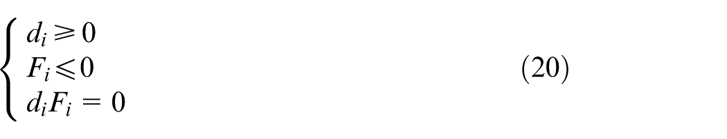
where d is the final distance between corresponding nodes, and F is the reaction force.
Step 3. A contact equilibrium search algorithm is used to calculate the reaction F and final distance d combined with conditions in step 2. Then the applied forces when building sensitive matrix in MIC are updated for clamping and welding parts. The assembly variation can be obtained considering of contact model.
Case study
Phased array antennas are widely used in many fields such as radar, communication and navigation. 29 The structure of phased array antenna can be divided into three layers: support layer, assembly layer and element layer, as shown in Figure 16. The whole phased array antenna is composed of a plurality of sub-arrays, and each sub-array contains several rigid and flexible parts. In this case, rigid errors at support layer and flexible errors at assembly layer of antenna sub-array are considered overall to make a variation analysis. Installation errors of transmitting terminals at element layer and position errors are neglected. Then the assembly variation of sub-array will be predicted.
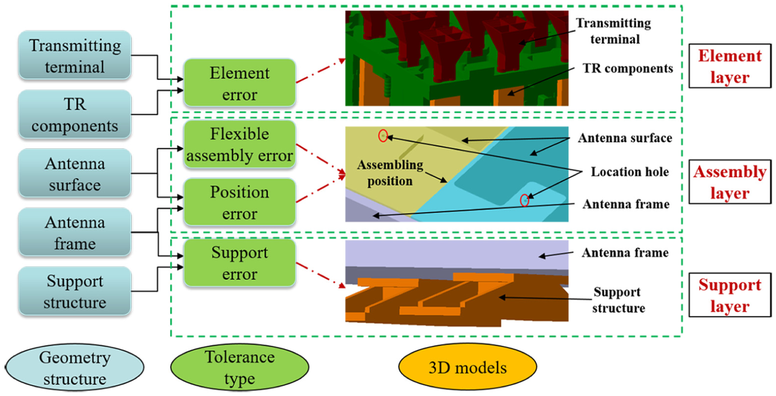
Structure of phased array antenna.
The structure of antenna sub-array is shown in Figure 17, in which base, wallboard, truss and support frame are rigid parts, and reflection plate is flexible part. Positions of array elements at element layer are influenced by assembly variation cumulated in sub-array, which will have an impact on antenna performance.
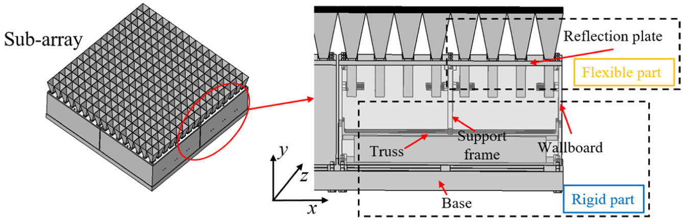
Structure of antenna sub-array.
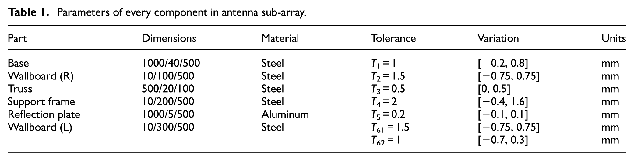
For the convenience of calculation, only parts’ manufacturing errors in the y-direction are considered. Parallelism of the upper surface of base is T1. Installation position error of truss and right wallboard along y-axis is T2. Truss has a parallelism of T3. Support frame has a size tolerance of T4. Shape tolerance of reflection surface is T5. Size tolerance and position tolerance of left wallboard are T61 and T62. The parameters of every component are given in Table 1.
Parameters of every component in antenna sub-array.
A vector loop composed of several structures in sub-array is constructed as in Figure 18. Vectors ri (i = 1, 2, 3, 4, 5, 6) are defined to describe each structure. For vectors of y-direction like r2, r4 and r6, their manufacturing errors are included in themselves. For vectors of x-direction like r1, r3 and r5, additional vectors k and f are added to represent their deviations in y-direction. View of vector-loop model in x–y plane is shown in Figure 18(a). Vectors fMi and fNi denote variables of discrete points on the reflector plate and the wallboard, respectively. Vectors k1s and k1e describe parallelism of base upper surface, which represent small variations of base sideline’s endpoints in y-direction. Similarly, k3e and k3m are description of truss parallelism, representing small variations of truss sideline’s endpoint and middle point in y-direction. According to the rigid–flexible hybrid vector-loop model in section “Construction of rigid–flexible hybrid vector-loop model,” vectors fMi and fNi are decomposed into corresponding components s and r, as shown in Figure 18(b).
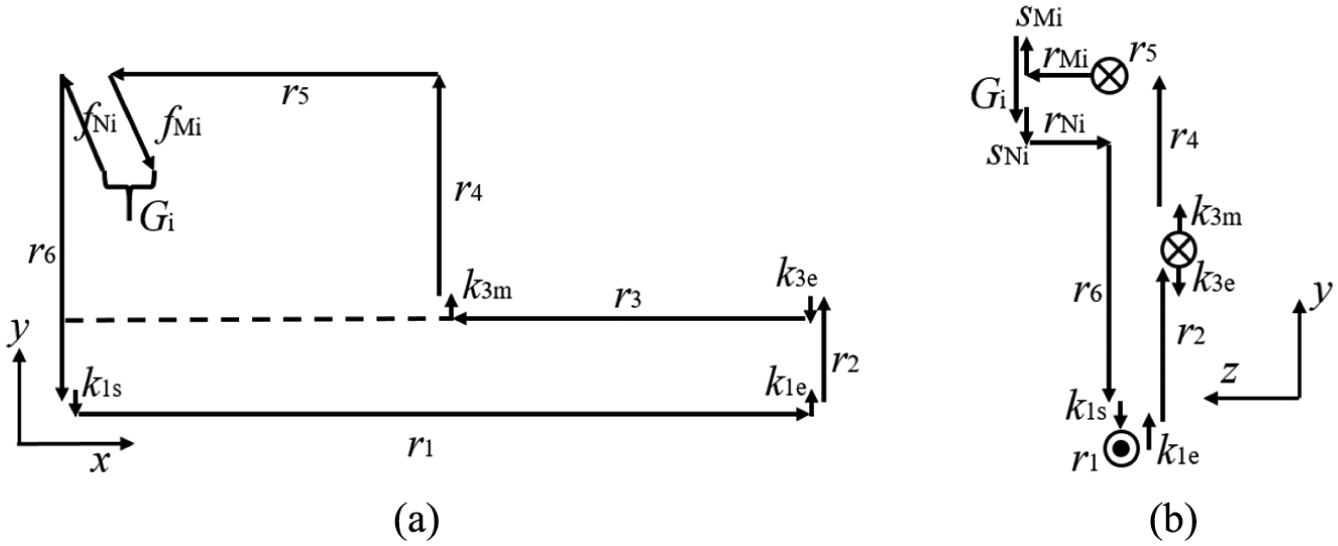
Vector-loop model of antenna sub-array: (a) view of x–y plane and (b) view of z–y plane.
As vector-loop model of antenna sub-array is constructed in Figure 18, gap of this product can be expressed as in equation (21). Coefficient matrices of gap to each vector are confirmed, and parameters in Table 1 are substituted to calculate the distances of every pair of corresponding discrete points
Combined with equation (16), variables of rigid size or position errors and flexible shape errors are listed as in equation (22)
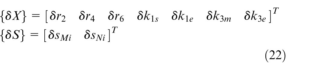
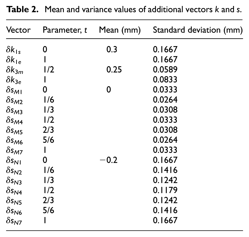
Additional vectors k and s are acquired based on statistical representation of discrete points on part surface based on skin model in section “Discrete statistical expression of part surface error characteristics.” Shape of reflection plate is assumed as a quadratic function surface. Seven discrete points are both sampled on reflection plate and wallboard sidelines uniformly. Means and variances of vectors k and s are calculated as in equation (23), where UD and LD, respectively, represent the upper and lower limits of part deviation. Substituting the tolerance values and variation intervals listed in Table 1, mean and variance values of additional vectors k and s are obtained as in Table 2
Mean and variance values of additional vectors k and s.
Since closed-loop structure and dependent variables {U} are not involved in this example, coefficient matrices
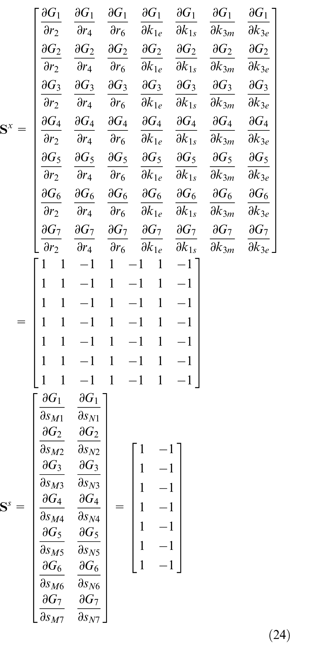
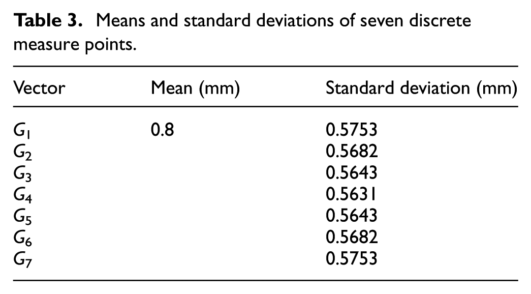
Then gap {G} between reflection plate and wallboard is calculated through equation (18) and means and standard deviations of seven discrete measure points are shown in Table 3.
Means and standard deviations of seven discrete measure points.
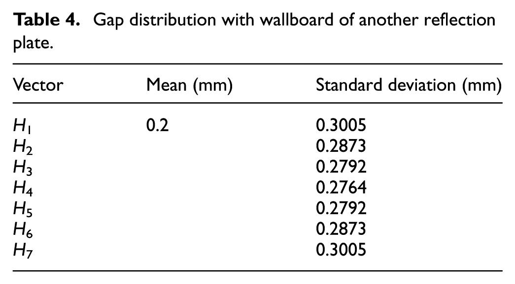
Suppose that another reflection plate to be assembled with this reflection plate has a corresponding gap distribution between the plate and wallboard in Table 4.
Gap distribution with wallboard of another reflection plate.
The reflection plate material is aluminum with a Young’s modulus E = 69 GPa, and Poison’s ratio ν = 0.35. Sensitivity matrix
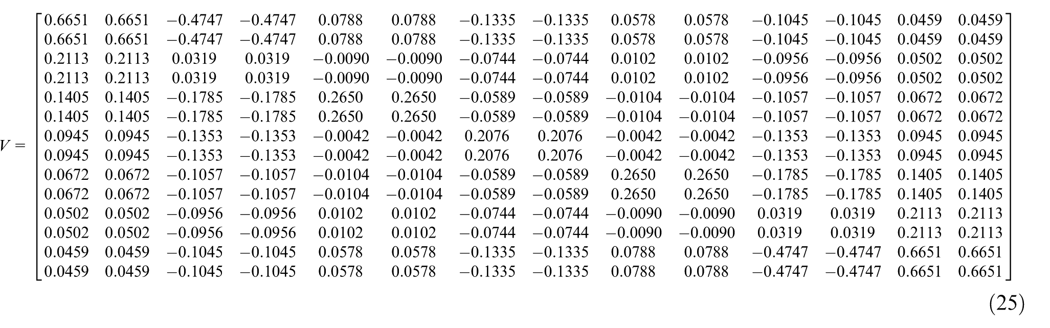
Means and standard deviations of measure points after assembly are shown in Table 5, through equations (19) and (25) with input parameters in Tables 3 and 4.
Means and standard deviations of measure points after assembly.
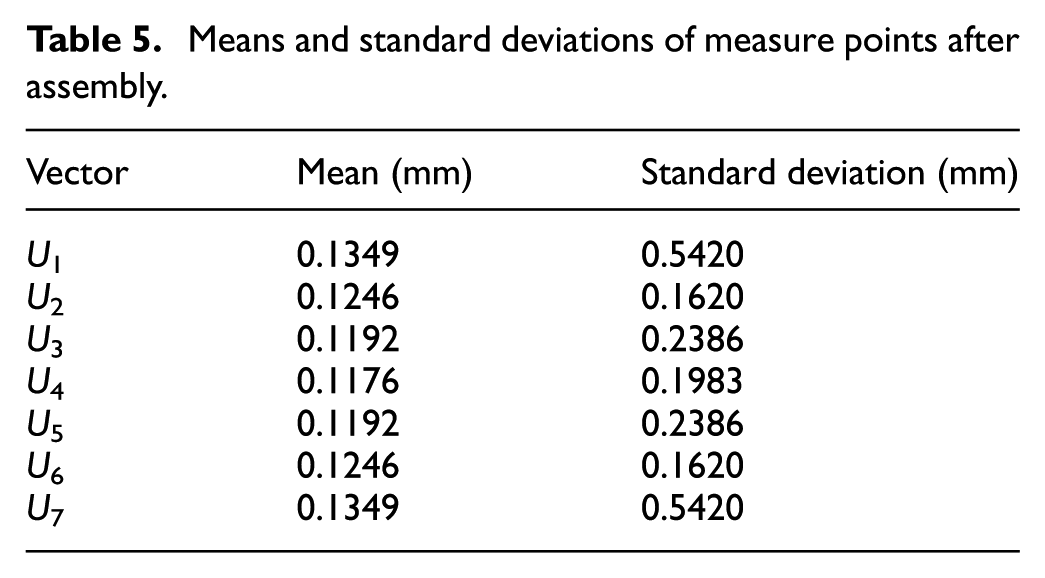
Figure 19 shows deformations of measure points whose node numbers are 12, 11, 23, 31, 30, 18, 17 under a certain circumstance in Abaqus® software.
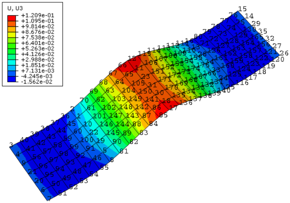
Deformations of measure points in Abaqus®.
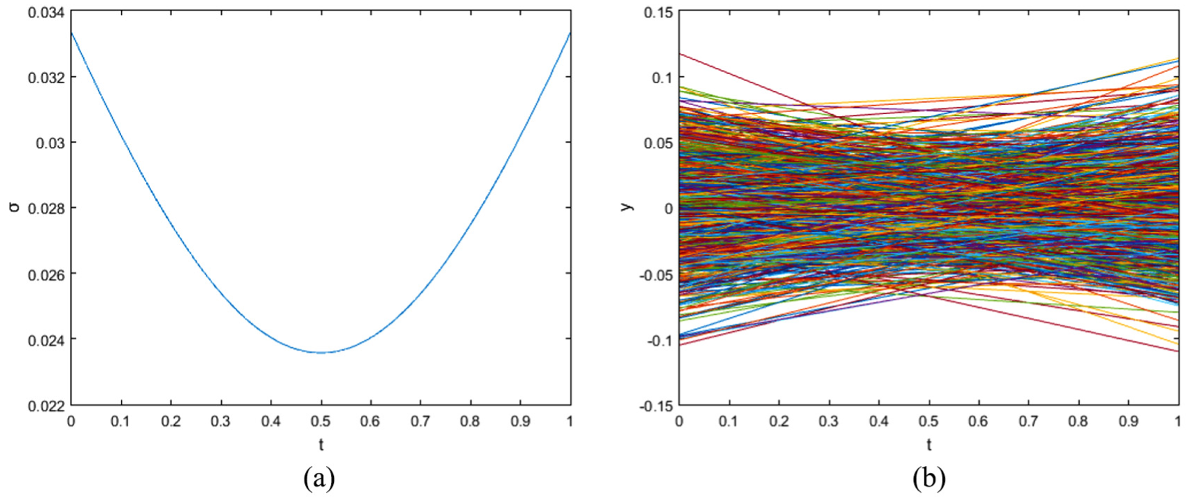
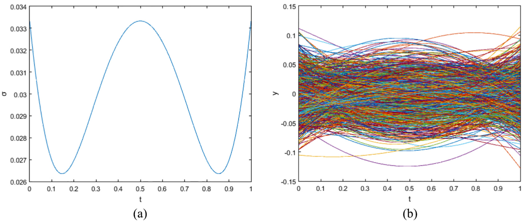
Figure 20 are graphical representation of data in Table 5 about mean and standard deviations of measure points after assembly. The rectangle of three colors is shown to describe lower boundary, mean value and upper boundary of measure points. From left to right in Figure 20, there are seven nodes corresponding to ones in Figure 19, whose numbers are 12, 11, 23, 31, 30, 18, 17. The attachment of upper boundary and lower boundary forms a closed envelope. And the actual assembly line has a 99.7% probability of falling within this range based on 3σ principle. The assembly success probability can be predicted compared with maximum allowed deformations.
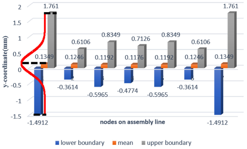
Mean and standard deviations of measure points after assembly.
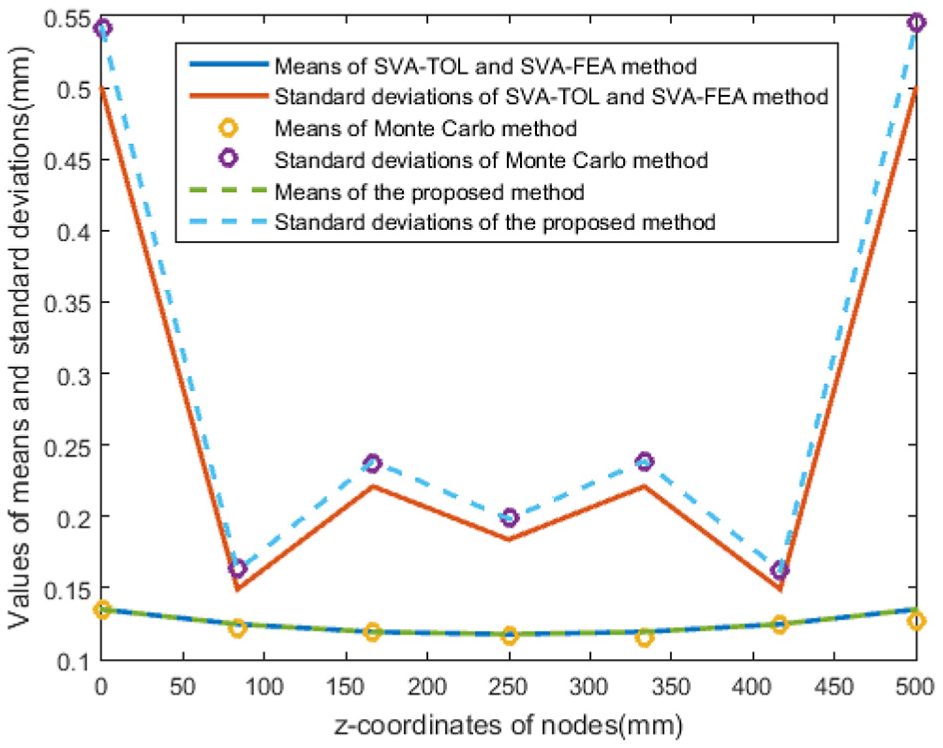
A comparison among traditional SVA-TOL and SVA-FEA method (represented by solid line), Monte Carlo method (represented by circles) and the proposed method (represented by dotted line) is made as shown in Figure 21. The result using Monte Carlo method is acquired by 104 sampling in parts’ manufacturing tolerance zones. It is regarded as a benchmark similar to experimental data. Traditional SVA-TOL and SVA-FEA method 22 is selected to calculate the mean and standard deviation of discrete points on assembly line. Means of three methods are [0.1352, 0.1247, 0.1193, 0.1174, 0.1193, 0.1247, 0.1352], [0.1344, 0.1222, 0.1194, 0.1165, 0.1155, 0.1243, 0.1371], [0.1349, 0.1246, 0.1192, 0.1176, 0.1192, 0.1246, 0.1349], and standard deviations of them are [0.4993, 0.1491, 0.2210, 0.1838, 0.2210, 0.1491, 0.4993], [0.5415, 0.1633, 0.2375, 0.1994, 0.2386, 0.1630, 0.5456], [0.5420, 0.1620, 0.2386, 0.1983, 0.2386, 0.1620, 0.5420], respectively. The units of mean and standard deviation are both millimeter. It can be seen that means of three methods have little difference, but standard deviations of the proposed method are closer to ones of Monte Carlo method, which has an approximate 8% accuracy improvement than traditional SVA-TOL and SVA-FEA method.
Comparison of traditional and proposed methods.
Conclusion
Aiming at existing insufficient in assembly variation analysis methods of complicated products, this article presents a method based on rigid–flexible hybrid vector-loop model. Flexible part vectors are described by a set of variables which are composed of discrete feature point errors according to tolerance types. Combined with traditional rigid part vectors, a uniform model of rigid–flexible hybrid vector loop is constructed. Probability density distributions of discrete feature points on part sidelines are characterized to represent rigid and flexible manufacturing errors. And final assembly deformations are predicted based on rigid–flexible hybrid vector loop and FEA.
The major contribution of this article is to connect the rigid and flexible variation analysis methods in an explicit way. It solves the variation propagation model including not only translation and rotation errors in rigid part but also shape error in flexible part. The unified variation model helps to obtain the weight coefficient of each manufacturing error to assembly variation, which is hardly come true by rigid or flexible variation analysis methods. Besides, through the comparison between proposed method and SVA method is made in case study, it is shown that our method has a more accuracy result than traditional method. That is significant for design and manufacture of rigid–flexible complicated mechanical products.
In further research, more factors will be analyzed for improving the proposed model, such as micro-level surface error and bolted connection. Meanwhile, assembly quality will be evaluated in terms of product performance rather than geometric assembly variation.
Footnotes
Declaration of conflicting interests
The author(s) declared no potential conflicts of interest with respect to the research, authorship and/or publication of this article.
Funding
The author(s) disclosed receipt of the following financial support for the research, authorship, and/or publication of this article: The author(s) disclosed receipt of the following financial support for the research, authorship, and/or publication of this article: This work was supported by the National Natural Science Foundation of China (Grant No. 51475418, 51490663, 51875517).