
Abstract
Three-dimensional tolerance analysis is increasingly becoming an innovative method for computer-aided tolerancing. Its aim is to support the design, manufacturing, and inspection by providing a quantitative analysis of the effects of multi-tolerances on final functional key characteristics and predict the quality level. This article proposes a novel approach for three-dimensional assembly analysis—a hybridization of vector loop and quasi-Monte Carlo method. The former is used to establish the three-dimensional assembly chain and obtain the assembly function. The latter is adopted to generate n sets of dimensional values according to the distribution of each dimension in chain. The new method is shown to inherit many of the best features of classical vector loop and quasi-Monte Carlo, combining easy-to-obtain assembly function with accurate statistical analysis. For every set of dimensional values, one sample value of a functional requirement can be computed with the Newton–Raphson iterative procedure. A crank slider mechanical assembly is shown as an example to illustrate the proposed method.
Keywords
Introduction
Three-dimensional (3D) tolerance analysis is hot focused for ever-tightening and increasing complex requirements in various fields. It enables the prediction of the cumulative effects of these part deviations on assembly and functional key characteristics. Tolerance analysis aims at not only improving the performance of a product but also reducing the cost.
A large amount of research has been devoted to two aspects in tolerancing domain: tolerance model and analysis method. Some models of 3D tolerance analysis are reviewed in detail and compared based on the literature published.1,2 A kinematic tolerance space model was proposed to express the relationship between the nominal kinematics of mechanisms and their kinematic variations. 3 The T-Map represents all possible variations in size, position, form, and orientation for a target feature by means of a hypothetical Euclidean point-space. 4 Mansuy et al. 5 applied deviation domain to perform both worst case and statistical tolerancing analysis. Similar to T-Map and deviation domain, the polytope represents geometrical deviations on mechanical parts by sets of half-spaces coming from the restriction of the position of a finite set of points of a toleranced feature. 6 Asante 7 used the small displacement torsor (SDT) model to analyze the combined effects of workpiece geometric error, locator geometric error, and clamping error on a machined feature. A proposed unified Jacobian–Torsor model combines the benefits for tolerance representation and propagation. 8 The skin model shape concept,9–11 developed from skin model theory,12,13 can be used for assembly simulation 14 and served as digital twin. 15 A gap-based approach, called GapSpace 16 that uses gap to describe the relationship between features belonging to different components, and three main sources of variations are included into vector-loop-based model for a mechanical assembly. 17 Some models have been integrated successfully into CAD packages for industrial environment, such as CATIA.3D FDT and FT&A are based on TTRS model and matrix model; CETOL 6 Sigma and Sigmund use vector-loop model; eM-TolMate, VSA, and 3DCS incorporate variational models; MECAmaster includes torsor model; and PolitoCAT and Politopix are developed based on polytope model. Currently, most of the CAD packages can deal with assemblies of varied complexities, among which CETOL 6 Sigma and Sigmund are able to consider part/assembly variation and kinematic motion for kinematic mechanisms due to the adoption of vector loop model.
The tolerance analysis methods are mainly worst case or statistical case. Statistical analysis is a more demanding way by permitting a small fraction of assemblies to not assemble or function as required, an increase in tolerances for individual dimensions may be obtained, and in turn, the manufacturing costs may be significantly reduced. 18 There exists root sum squared (RSS) method, 19 system moments, 20 Taguchi’s method, 21 the iterative method, 22 product of exponentials, 23 and Monte Carlo simulations24–27 for statistical tolerance analysis. In particular, the Monte Carlo method is the most widely used method in statistical tolerance analysis as it allows the use of normal and non-normal distributions, as well as linear and nonlinear assembly functions. The CAD packages, such as CETOL 6 Sigma, VSA, eM-TolMate, 3DCS, Mechanical Advantage, Sigmund, and RD&T, are able to use Monte Carlo to perform simulations. However, this method requires a large number of samples to assure accuracy. Motivated by this shortcoming, a so-called good point set of quasi-Monte Carlo method was used to generate samples of the dimensions. 28 This method resembles Monte Carlo in applications that are suitable for either normal or non-normal input/output, and linear or nonlinear assembly functions. The difference between these two methods lies in the fact that the quasi-random numbers generated for quasi-Monte Carlo have a lower discrepancy than that generated by the Monte Carlo method, and therefore fewer samples are necessary to guarantee accuracy. Previous work presented for quasi-Monte Carlo focused on mechanical assembly with explicit objective function. 28 To promote the applicability of the method in tolerancing domain, the vector loop is introduced, which is an innovative category of tolerance analysis method that three main sources of deviations in a mechanical assembly are fully considered.29,30 The direct linearization method (DLM), the second-order tolerance analysis (SOTA), and the Monte Carlo method have been developed to derive the functional requirement in vector loop model. Nevertheless, DLM may be inaccurate for highly nonlinear assemblies, and SOTA is an approximation due to the approximation of the three sets of partial derivatives in every iteration while Monte Carlo requires large computations. In this regard, an approach is proposed for 3D assembly tolerance analysis which seeks to combine the benefits of the classical vector loop and quasi-Monte Carlo. The new approach is designed to describe the implicit assembly function consistent with vector loop scheme, while also inheriting the sample strength of quasi-Monte Carlo. This novel method is an extended work of quasi-Monte Carlo in tolerance analysis.
The rest of the article is organized as follows. Section “Vector-loop-based assembly function” illustrates the representation of the assembly function. Section “Newton–Raphson iterative method” proposes a solution toward to solving the assembly function. Section “Dimension sample method” describes the quasi-Monte Carlo method for generating samples. Section “3D tolerance analysis method” presents the overall 3D tolerance analysis process. A 3D mechanism is presented to verify the validity and accuracy of the proposed method in section “Case study.” Finally, section “Conclusion” provides the conclusions.
Vector-loop-based assembly function
An assembly dimension chain can be described as a closed vector loop. In two-dimensional (2D) space, the vector loop equation results in three scalar equations, representing the sum of the x and y projections of the dimension vectors in global coordinates and the sum of the relative rotations. However, in 3D space, the projection equations still hold in global x, y, and z, but the rotation constraints can only be expressed in matrix form. A vector loop that contains m vectors
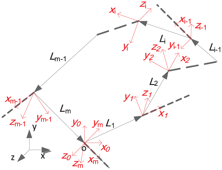
Vector loop and local coordinate systems.
A closed 3D loop can be expressed in terms of a concatenation of coordinate transformation matrices as shown in equation (1). Equation (1) describes that the coordinate system at the end of the loop must be truly the same as the coordinate system at the beginning
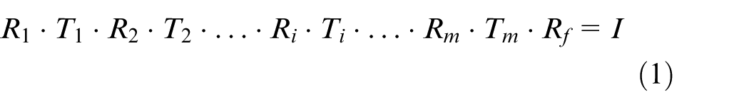
where
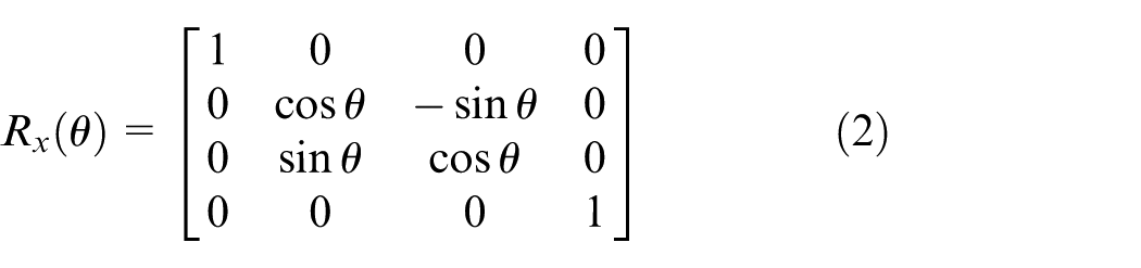
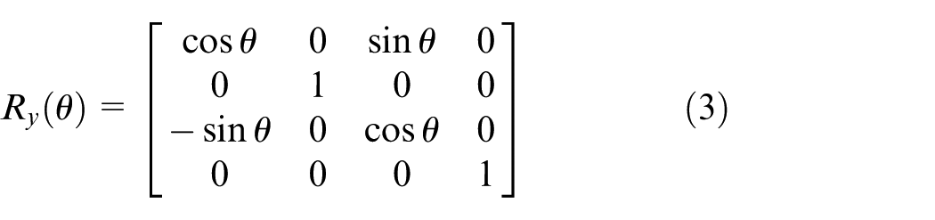
To describe the loop equation in matrix form, four elementary homogeneous transform matrices, as shown schematically in Figure 2, are used.
The
The
The
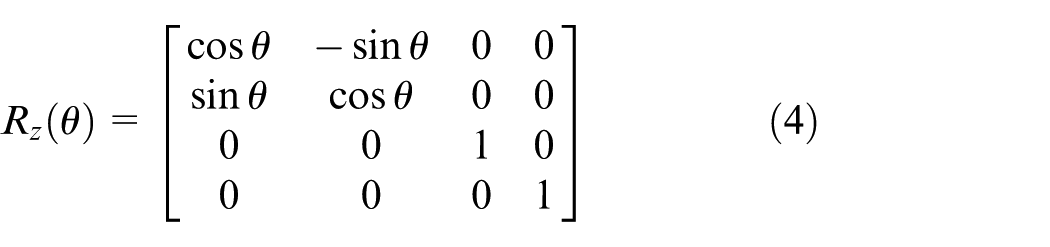
The
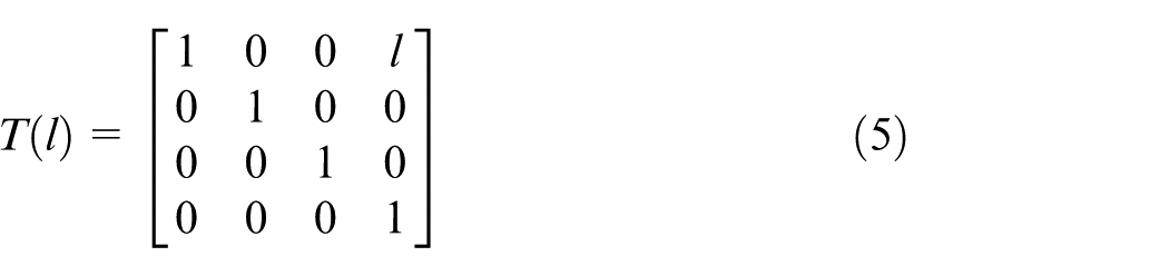
Three-dimensional representations for the four elementary matrices (a) Rotation around the x axis, (b) rotation around the y axis, (c) rotation around the z axis and (d) translation along the x axis.
With this convention, the vector loop equation (equation (1)) can be expressed in matrix form, therefore, forming the necessary assembly function. This method is well capable of obtaining assembly function on occasions that are difficult or impossible to calculate explicit function.
Newton–Raphson iterative method
For a general 3D assembly, the functional requirement is expressed as a nonlinear function of the dimensions and constants of the assembly, and it is difficult to solve this equation for a general case. The nonlinear equation requires a nonlinear solver to find solution. Since Newton–Raphson method has the best convergence rate of nonlinear system solvers, in this section, the method is adopted to solve the equation. In this regard, the iterative formula is mostly required. Before the iterative formula is deduced, derivatives of the elementary matrices and partial derivatives of function
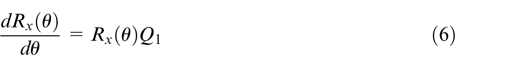
Derivatives of the elementary matrices
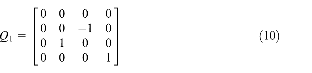
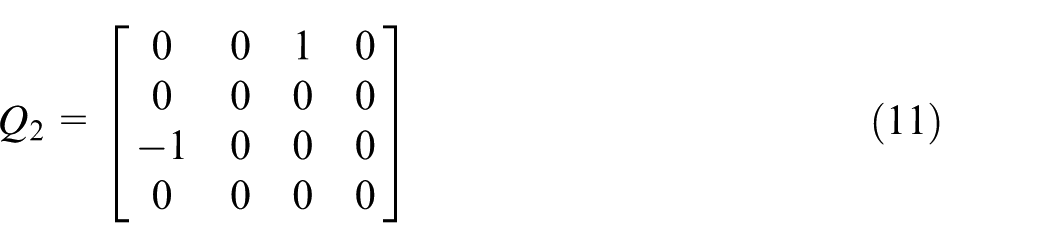
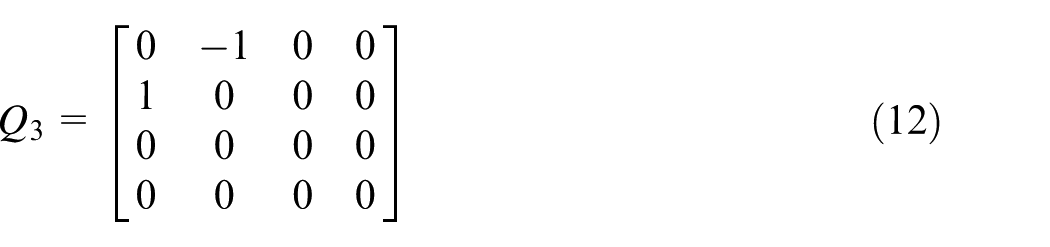
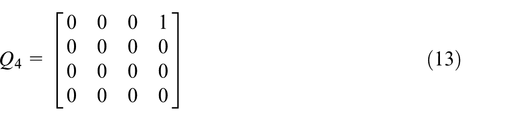
It is mathematically convenient to describe the operation of taking the derivative as a matrix product. Define the derivatives of the elementary matrices as follows
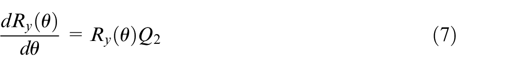
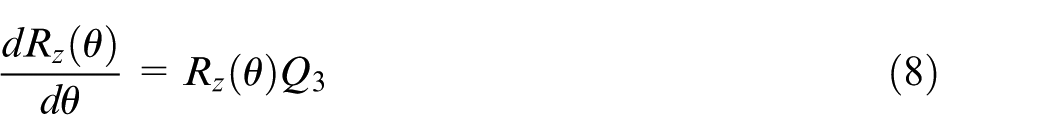
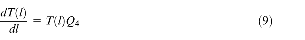
where
Partial derivatives of function S (q )
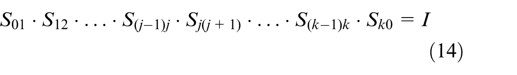
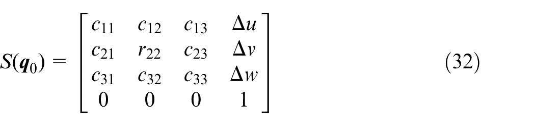
For convenience, equation (1) is rewritten as equation (14). It is important to note that
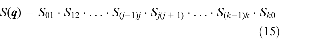
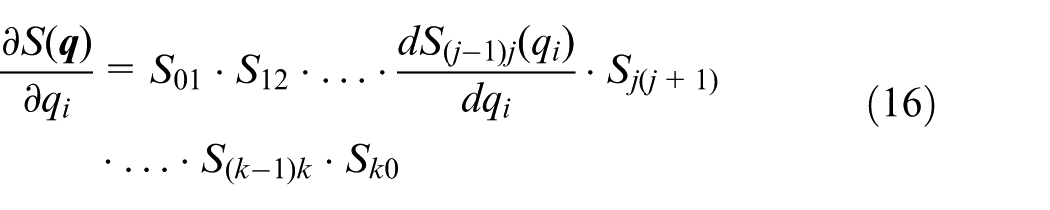
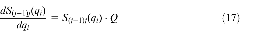
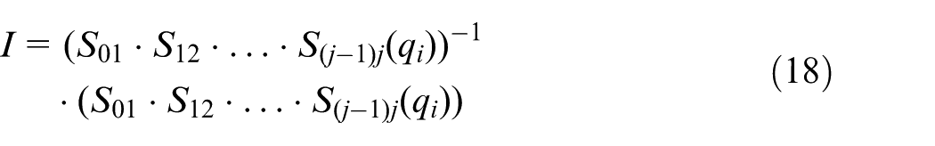
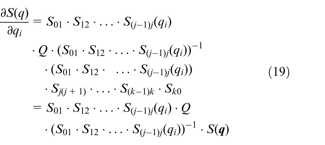
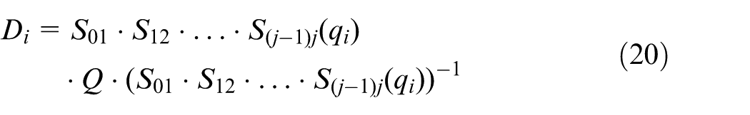
For a 3D assembly, there exist six unknown dimensional variables or assembly variables. Define the left-hand side of equation (14) as a function depicted in equation (15), then the derivative of which can be represented as equation (16). Because of the existence of equations (17) and (18), equation (16) changes into equation (19).
where
where Q is the proper type of derivative operator matrix for the elementary matrix
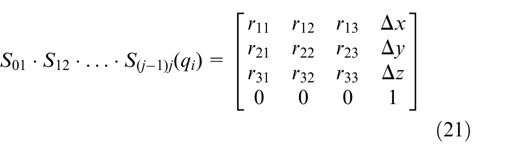
For simplifying calculation purpose, we assume
where
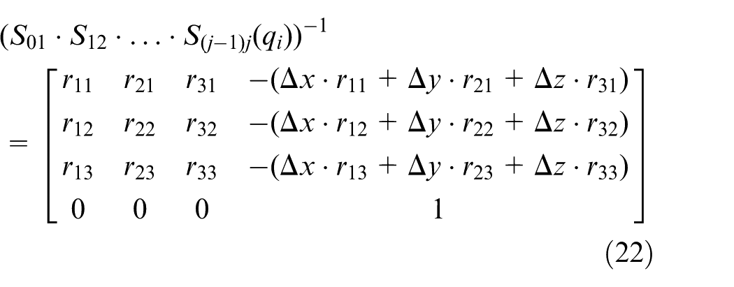
where
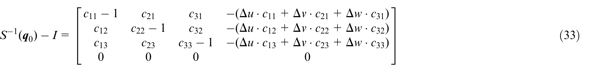
If
If
If

If
Iterative formula
According to equations (14) and (15), the assembly function can be rewritten as

To solve the assembly function in equation (27), a Newton–Raphson iterative procedure is carried out. First, an initial value
The first-order linear expansion of equation (27) about
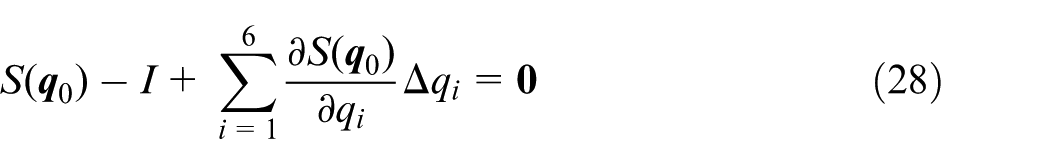
As per equations (17)–(20), equation (28) becomes
Post-multiplying by
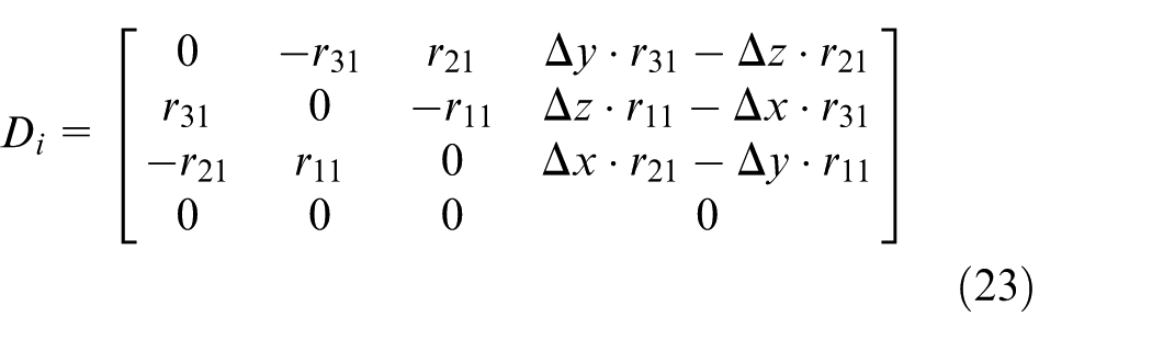
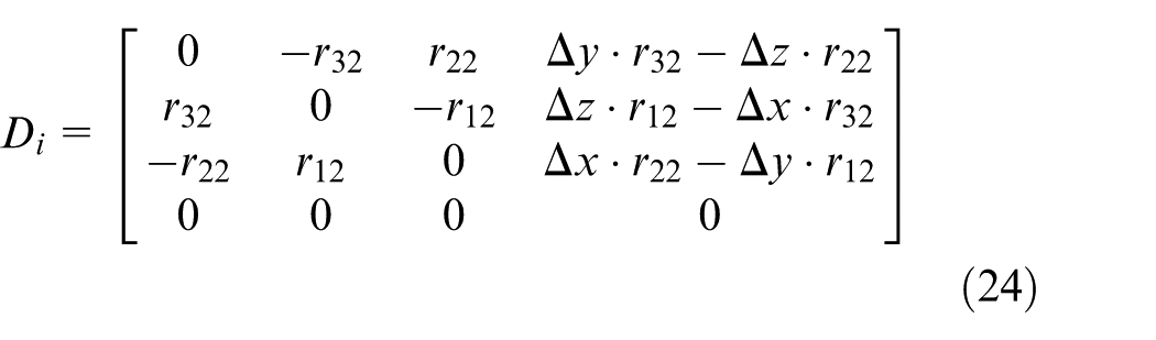
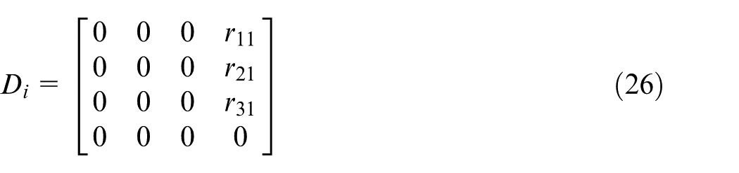
According to equations (23)–(26), a general form of
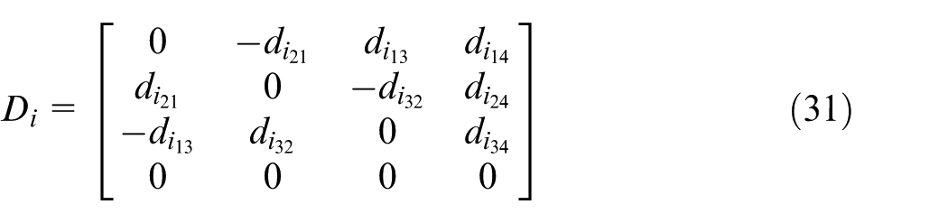
It is obvious that only
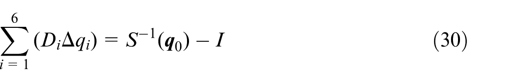
For the right-hand side of equation (30),
where
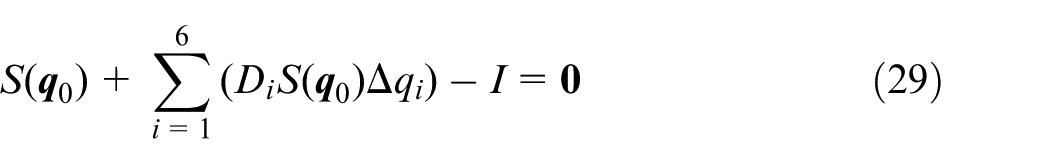
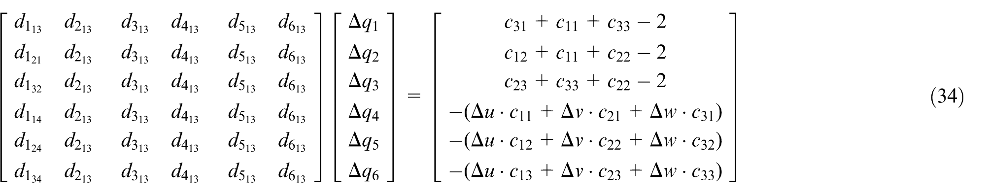
In summary, the scalar equations for the iteration procedure can be written in matrix form as expressed in equation (34)
Therefore, the small variation can be obtained as follows

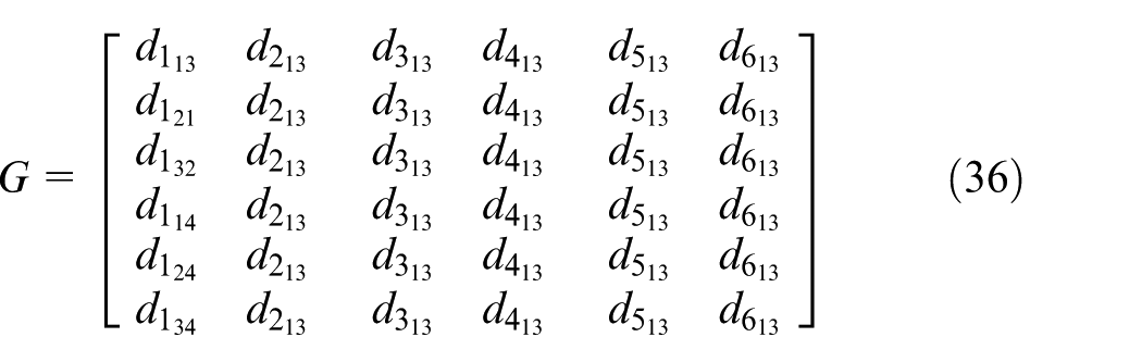
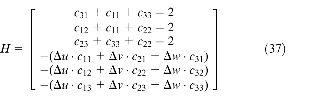
where
Dimension sample method
After obtaining the matrices G and H, a quasi-Monte Carlo method is adopted to generate the manufacturing variables.
Take

where
Take

Take p as a prime and

Take p as a prime and
Figure 3(a) and (b) shows the point sets generated by the Monte Carlo method and the quasi-Monte Carlo method. It is obvious that the good point set generated is only decided by s, which represents the number of manufacturing variables. For an assembly, it is easy to obtain the certain variables by creating the vector loop. Therefore, the generated good point set is fixed. It should be mentioned that if
(a) Points generated by Monte Carlo method and (b) points generated by quasi-Monte Carlo method.
After the good point set is obtained, an inverse transformation method can be used for generating an observation from a given distribution. The natural idea for generating random variables
Generate a good point set
Take
Use
3D tolerance analysis method
In this article, a quasi-Monte Carlo method is used to generate n sets of dimensional values according to the distribution of each dimension. By defining the iterative formula, one sample value for the functional requirement can be computed following the Newton–Raphson iterative procedure. Finally, the first four order moments of the function requirement can be computed after n samples of the function requirement are found and thus the assembly reject can be estimated. A flow diagram of the proposed method is shown in Figure 4. The input information includes the probability distributions of the dimensions, the nominal value and tolerance of the functional requirement, and the nominal values of the assembly variables.
Flow diagram of the proposed method.
After creating the local coordinate systems, the assembly function can be derived, as shown in section “Vector-loop-based assembly function.”
The quasi-Monte Carlo method is presented to generate a sample of the dimensions. The number of dimensions is s. Let p be a prime and
where
Then, the points

where
After generating the sample of dimensions, the Newton–Raphson iterative procedure is used to obtain a sample of the functional requirement. Standard statistical estimation methods are then used to compute the first four order moments of the samples. Finally, the assembly reject is estimated by integration or a table.
Case study
The performance of the proposed method was investigated experimentally, with techniques used to analyze the benchmark mechanism. A 3D crank slider mechanism that consists of a base, a crank, a link, and a slider will be used. The vector loop, local coordinate systems, and the dimensions which govern the operation of the 3D assembly are shown in Figure 5. The assembly reject associated with U due to manufacturing variations is the key issue to determine the assemblability.
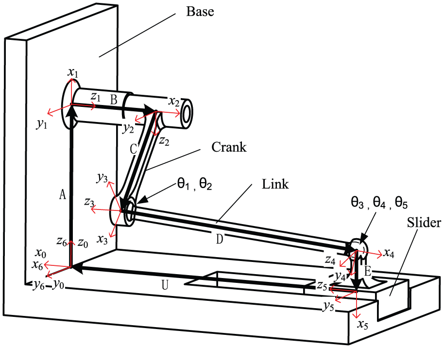
Vector loop and local coordinate systems.
The proposed method consists of the following steps:
Step 1. Identify the variables. The independent manufacturing dimension variables are A, B, C, D, and E, whereas the distance U and angles
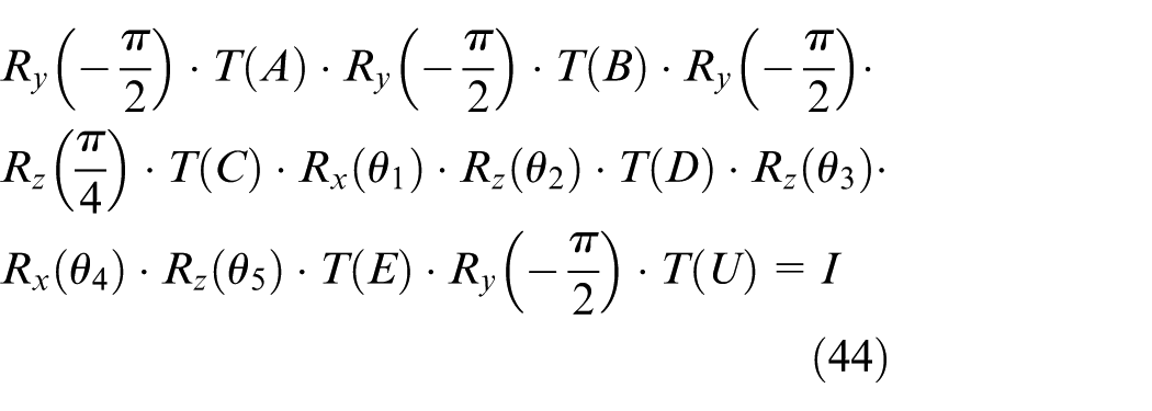
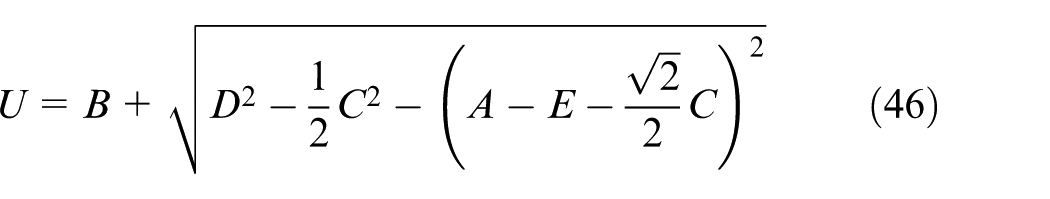
Step 2. Obtain the assembly function. The vector-loop-based assembly function can be expressed as
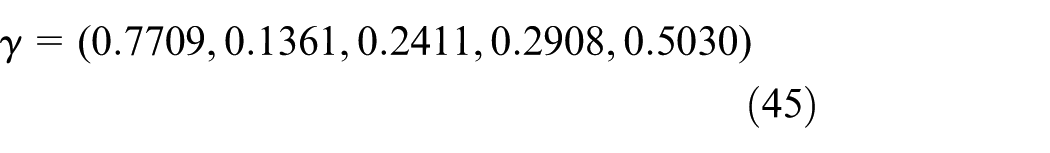
Step 3. Calculate the G and H matrices. The sample of dimensions A, B, C, D, and E can be represented by good point set. Here,
Detailed dimensions for the 3D assembly.
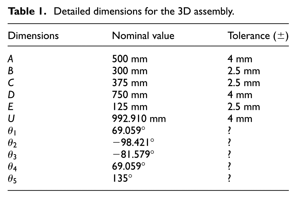
For every sample of A, B, C, D, and E, a sample of the distance U and angles
Step 4. Compute the mean and standard deviation through statistical formulas, and the assembly reject is estimated by integration.
Step 5. For comparison purpose, the conventional Monte Carlo method in vector loop model was performed, allowing its output to be compared with the proposed method side-by-side. Due to similarities in the overall analysis framework, a common procedure was used, differing only in the generation approaches of random variations.
To provide additional performance information, the result obtained from the explicit assembly function is included in a subset of comparisons. The explicit assembly function is expressed as
The various numbers of sample by Monte Carlo and quasi-Monte Carlo were proceeded. Detailed statistics on analysis results are presented, including mean and standard deviation of the functional requirement. As shown in Figures 6 and 7, overall, the novel method gives a smaller scope of variations with improved sample efficiency to be stable compared to the Monte Carlo method. Focusing on the distribution of the mean, it can be seen that the proposed method has moderate amplitude and becomes stable when n is greater than 500, while Monte Carlo method varies in a more acute sense and stays stable after 600 samples. In terms of standard deviation, the proposed method is seen to achieve significant improvements for keeping relatively small values. In addition, the sample size is smaller when the standard deviation stays steady for the proposed method with respect to the conventional vector loop method. Besides, due to the reusable characteristic of sample strategy in this study, only excessive samples need to be newly generated as sample size increases, which practically reduces the computation efforts.

Comparison of the means.
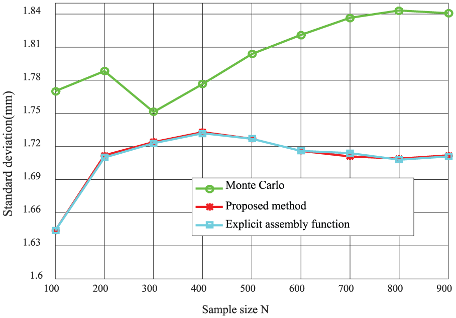
Comparison of the standard deviations.
The comparison between the proposed method and the explicit assembly function method is then performed, as shown in Figures 6 and 7. The results obtained by the proposed method are almost the same as those from the method using an explicit assembly function to obtain the samples of U. Besides, the relative error of mean given by the proposed method is small with a low relative error of the standard deviation, which is less than 1000, indicating the effectiveness and accuracy of solving the implicit assembly function by the presented method. As per Figure 7, when the sample size n reaches 800, the standard deviation of the samples is −0.146%, to a minimum. Simultaneously, the relative error of the mean is as low as 0.001%, in which the comparison object for the relative error is the value of the previous sample. The mean and standard deviation have reached their comparatively stable values. In this regard, the mean and standard deviation associated with the 800 samples size can be used to estimate the assembly reject and the result is 1.924%.
Conclusion
The attempt of the presented work is to propose a novel 3D tolerance analysis method for assembly. The new method is based on the quasi-Monte Carlo algorithm, which had been developed to use low-discrepancy point set to statistically analyze the assembly with explicit objective function.
In this study, this work has been extended to support implicit assembly function through the integration of the vector loop model. This new scheme is a hybrid approach that combines the advantages of conventional quasi-Monte Carlo and vector loop techniques. The vector loop is used to obtain the assembly function, and quasi-Monte Carlo is used to generate samples of the dimensions for statistical analysis. The presented method solves the difficulty of obtaining implicit assembly function, as well as calculating vector-loop-based objective function. The method has shown its validity and accuracy via a 3D assembly analysis. However, in future research, the geometric tolerances will be taken into account and developments will concern complex assembly with multiple loops.
Footnotes
Declaration of conflicting interests
The author(s) declared no potential conflicts of interest with respect to the research, authorship, and/or publication of this article.
Funding
The author(s) disclosed receipt of the following financial support for the research, authorship, and/or publication of this article: This research was supported by the National Natural Science Foundation of China (NoS. 51575484 and U1501248) and the Science Fund for Creative Research Groups of National Natural Science Foundation of China (No. 51521064).