
Abstract
The demands for advanced and flexible docking equipment are increasing in the fields of aerospace, shipbuilding and construction machinery. Position and orientation accuracy is one of the most important criteria, which would directly affect the docking quality. Taking a novel one-translational and three-rotational docking equipment, referred to as PaQuad parallel mechanism as example, this article proposed an accuracy improvement strategy by geometric accuracy design and error compensation. Drawing mainly on screw theory, geometric error modeling of PaQuad parallel mechanism was first carried out via four independent routes. Joint perturbations and geometric errors were included in each route error twist. Wrenches due to articulated traveling plate were applied to eliminate joint perturbations. Then, geometric accuracy design was implemented at component and substructure levels. The basic principle was to transfer geometric errors into dimensional or geometric tolerance. High-precision machining/assembling techniques were applied to satisfy the tolerance. Finally, error compensation resorting to kinematic calibration was implemented at mechanism level. It can be summarized as identification modeling, measurement planning, and parameter identification and modification. Maximum deviations of PaQuad parallel mechanism before calibration experiment were 0.01 mm,
Keywords
Introduction
Advanced and flexible docking equipment is highly required for high-precision assembling of large-scale components. This increasing demand has become a primary concern in the fields of aerospace, shipbuilding, and construction machinery. 1 Among various topology structures of docking equipment, parallel mechanisms (PMs) have been recognized as the most promising solutions due to their advantages in stiffness, dynamics, and accuracy.2–5 Geometric accuracy is one of the fundamental and challenging problems for PMs to the application of docking equipment. Taking a one-translational and three-rotational (1T3R) PM (named “PaQuad PM”) as example, the efficient method to improve geometric accuracy was investigated in this article.
Geometric accuracy of PMs has been intensively studied in the past few decades. It can be roughly divided into two strategies, that is, geometric accuracy design 6 and error compensation.7,8 Geometric accuracy design tries to obtain precise component and substructure through high-precision machining and assembling techniques. Resorting to kinematic calibration, error compensation is to identify and modify geometric errors after the PM was built. 9 There have been large numbers of researches focusing on kinematic calibration because of its economical and efficient features.10–12 However, it is found that kinematic calibration cannot achieve the best compensation if component or substructure was not properly designed. Thus, improving geometric accuracy of PMs from both accuracy design and error compensation is necessary.
Prior to geometric accuracy design and error compensation, geometric error modeling is required. Up to present, three main methods have been adopted for geometric error modeling, that is, Denavit–Hartenberg (D-H) convention, product of exponential (PoE) formula, and screw theory. D-H convention and its variants are popular among serial manipulators due to its simplicity and convenience.13–15 However, it cannot solve near-singular problem and little structural change may lead to the failure of error modeling.16,17 On the basis of Lie group theory, PoE formula applies line geometry to describe joint axes. The smooth exponential mapping from Lie algebra se(3) to Lie group manifold SE(3) can deal with kinematic singular problems. 18 But the formulation of error modeling becomes complicated when PM was taken into account. On the contrary, joint axis can be expressed by screw theory in a clear and concise manner,19–22 which is convenient for describing geometric error transmission. And geometric error model can be easily formulated through reciprocal product of twist and wrench.23,24 Hence, screw theory–based approach has been widely accepted in the error modeling of PMs, for instance, 5 degree-of-freedom (DoF) machine tools.8,25 Herein, screw theory is adopted for the geometric error modeling of PaQuad PM. However, different from single platform of common PMs, articulated traveling plate (ATP) of PaQuad PM is composed of two in-parts and one out-part. 26 Additional rotation can be obtained by relative movements among in-parts. How to properly consider the effect of ATP in error modeling was one of the difficulties in this article.
Based on geometric error model, geometric errors can be restrained by geometric accuracy design at component and substructure levels. Some basic principles would be proposed to guide the machining and assembling processes in this article. With the acceptable accuracy provided by geometric accuracy design, kinematic calibration is then implemented for compensating geometric errors at mechanism level.7–12 Kinematic calibration is the combination of theoretical analysis and experimental technique. It can be divided into three steps, identification modeling, measurement planning, and parameter identification and modification.
The main obstacle in identification modeling is ill-conditioning problem caused by approximately linear dependent identification vectors. To solve this problem, various methods have been proposed, such as, least square algorithm, 27 Levenburg–Marquardt algorithm, 28 genetic algorithm, 29 or Kalman filtering approach. 30 Although these methods are effective in dealing with ill-conditioning problem analytically, they are not efficient enough for mechanisms similar to PaQuad PM. An intuitive way is to directly solve the ill-conditioning equations. With this concept, Huang et al. 31 successfully found the solution for inverse identification equation of 3-PRS PM by regularization method. Herein, P, R, S denote actuated prismatic joint, revolute joint, and spherical joint. Based on Huang’s work, ridge estimation combining with L-curve selection 32 was adopted in this article for more stable and efficient identification modeling.
Measurement planning tries to achieve the best calibration results with least measuring configurations. For this purpose, external measurements by means of high-precision measuring equipment have been widely accepted: for instance, ball-bar system Hexapod 33 and redundant 2-DoF PM, 34 magnetic tooling balls for planar 5R PM, 35 visual method for Delta PM 36 and industrial robot, 37 and laser tracker for 5-DoF machine tool. 9 External measurement can be divided into partial and complete measuring schemes.38–40 Partial measuring scheme is able to derive optimized measurements by ignoring some DoFs. But additional algorithm might be required for identifying all geometric errors. And the measuring process is not general since different PMs correspond to different partial measurements. Comparing with partial measuring scheme, complete measuring scheme is easier to implement and the comprehensive measuring data simplifies identification process. It is applicable for all sorts of PMs, including PaQuad PM.
Parameter identifying and modifying is to carry out calibration experiments resorting to identification model and measurement plan. 41 By going through all measuring configurations, geometric errors are identified by identification model. Finally, they are compensated by adjusting inputs or modifying kinematic parameters in the control system. 42
Overall, accuracy improvement strategy proposed in this article can be summarized as (1) geometric error modeling between all possible geometric errors and errors of PM based on screw theory, (2) geometric accuracy design at component and substructure levels, and (3) error compensation resorting to kinematic calibration at mechanism level, including identification modeling, measurement planning, and parameter identification and modification (see Figure 1).
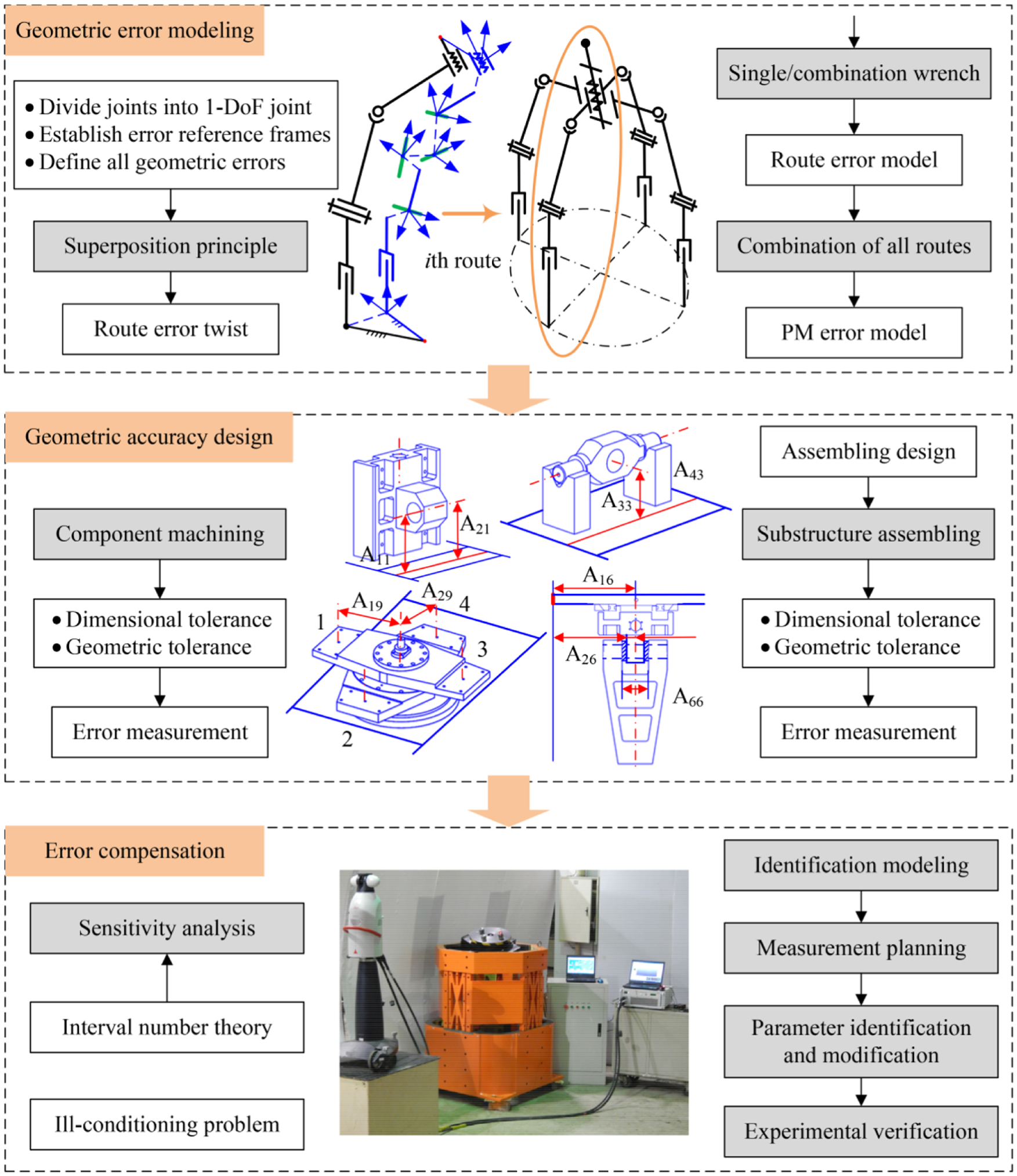
Accuracy improvement procedure of PaQuad PM.
Taking PaQuad PM as an example to demonstrate the accuracy improvement method, this article is organized as follows. Section “Geometric error modeling” formulated geometric error modeling of PaQuad PM. Some principles for geometric accuracy design were proposed in section “Geometrical accuracy design,” while kinematic calibration was implemented in section “Error compensation.” Section “Experimental verification” carried out experimental verification. And conclusions were drawn in section “Conclusion.”
Geometric error modeling
As is shown in Figure 2, PaQuad PM 1 is composed of fixed base, ATP, and four identical PRS limbs. The PRS limbs link to ATP and fixed base with S joint and P joint. The axis of P joint is vertical to the plane of fixed base. ATP consists of in-part 1, in-part 2, and out-part. In-part 1 and in-part 2 connect to out-part by H joint and R joint. Herein, axes of the two joints are collinear and H denotes helical joint. PaQuad PM has 4 DoF in terms of 1T3R, and its detailed DoF analysis can be seen in Song et al. 1 and Sun et al. 26
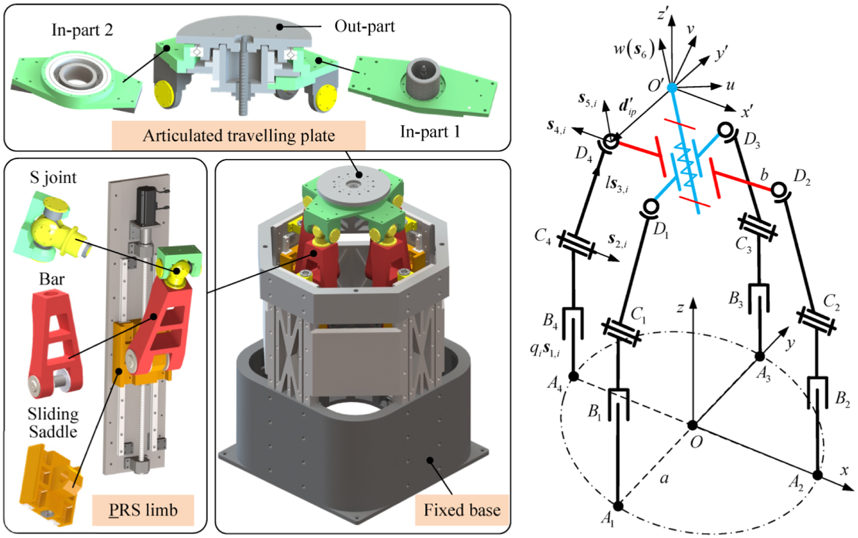
Virtual prototype and schematic diagram of PaQuad PM.
Some denotations were given in the schematic diagram as shown in Figure 2. The plane of fixed base was formed by point
For PaQuad PM, there were four independent routes to transmit geometric errors from fixed base to end reference point, ith
Note that error twists of the four routes were similar. First PRS limb plus ATP was selected as an example to demonstrate the error modeling process. As is shown in Figure 3, error reference frame
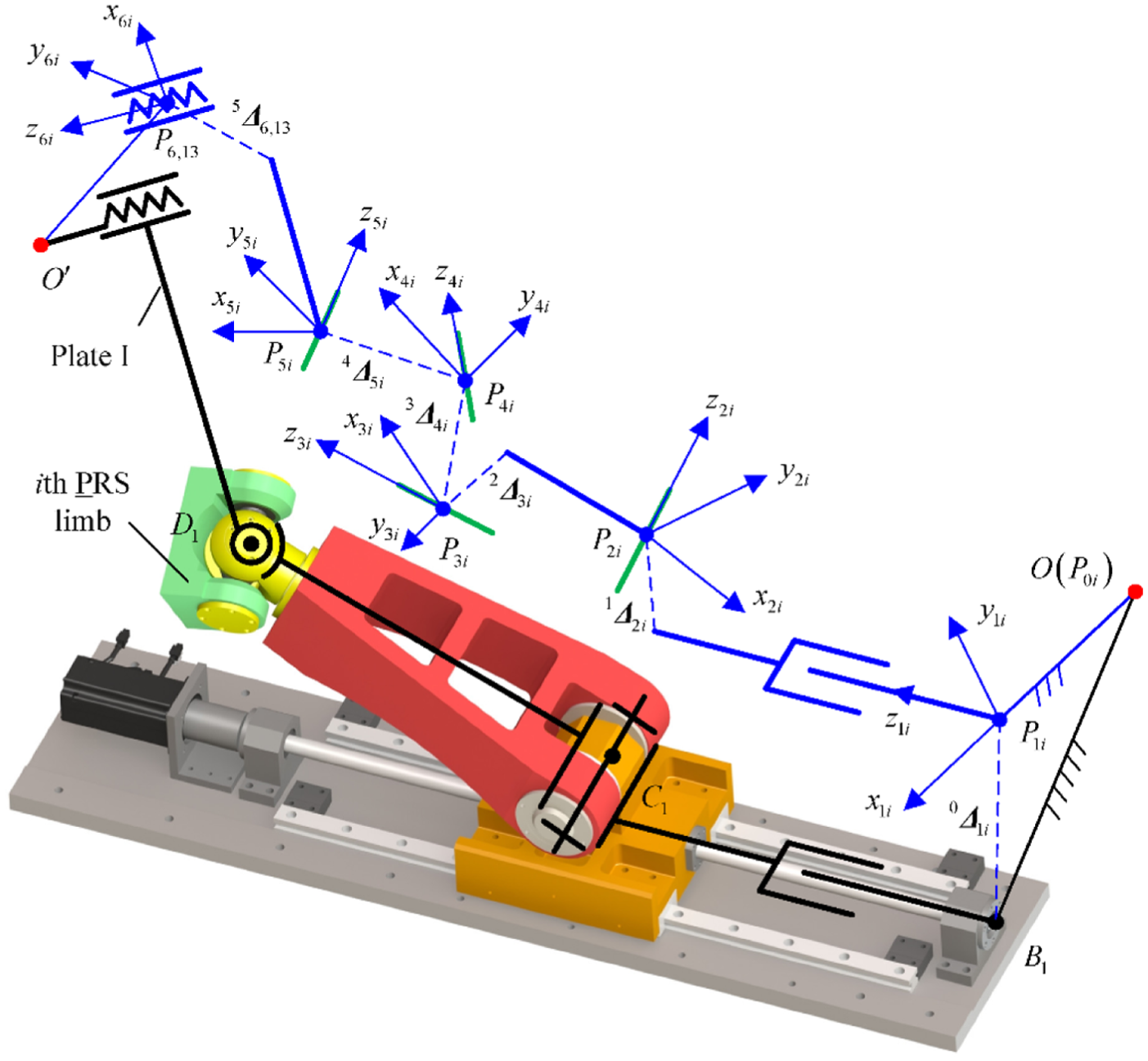
Geometric errors of first PRS limb plus ATP.
According to the defined error reference frame, transformation matrices between frames can be calculated as
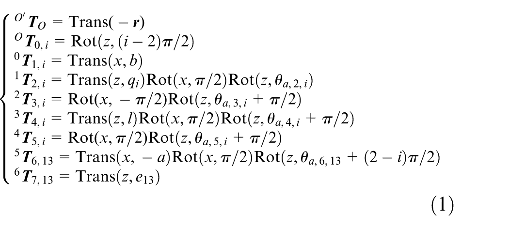
Herein,
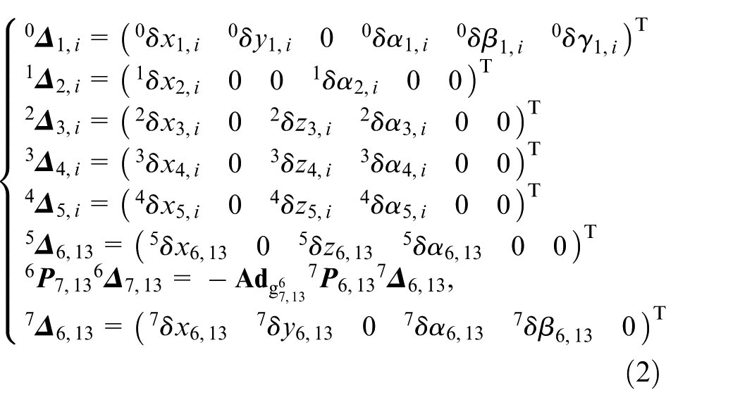
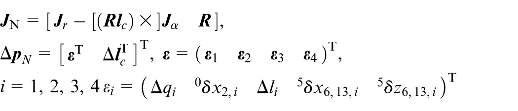
Based on screw theory, the route error twist was obtained by the superposition of all possible geometric errors and joint perturbations in frame
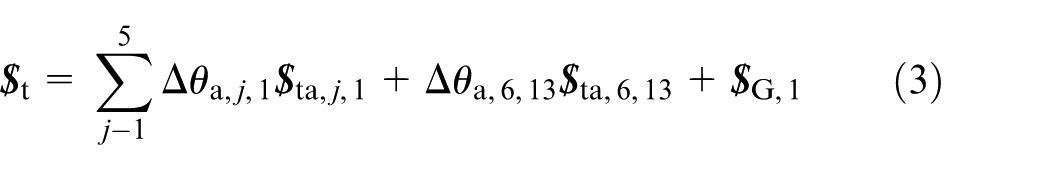
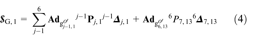
where
Taking ATP into account, wrenches of PaQuad PM can be divided into two types: single wrench provided by each route and combination wrench provided by combined effects of opposite routes. 1 In order to eliminate joint perturbations, reciprocal product of error twist and wrenches were applied to equation (3). When single wrench was applied, it turned out that
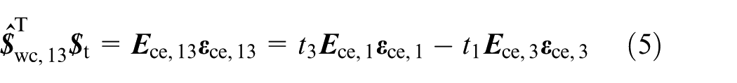
where
When combination wrench was applied, the reciprocal product yielded to
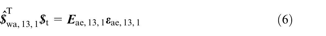
where
Therefore, geometric error model of first PRS limb plus ATP can be formulated by combining equations (5) and (6). With the same manner, the error models of other three routes were obtained.
After deleting repetitive geometric errors and modifying corresponding coefficients in the four error models, error model of PaQuad PM was achieved by combining error models of the four routes into matrix form as follow

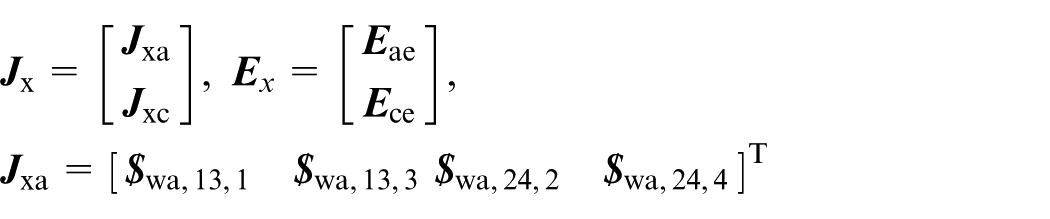
The modified error coefficient matrix
Geometrical accuracy design
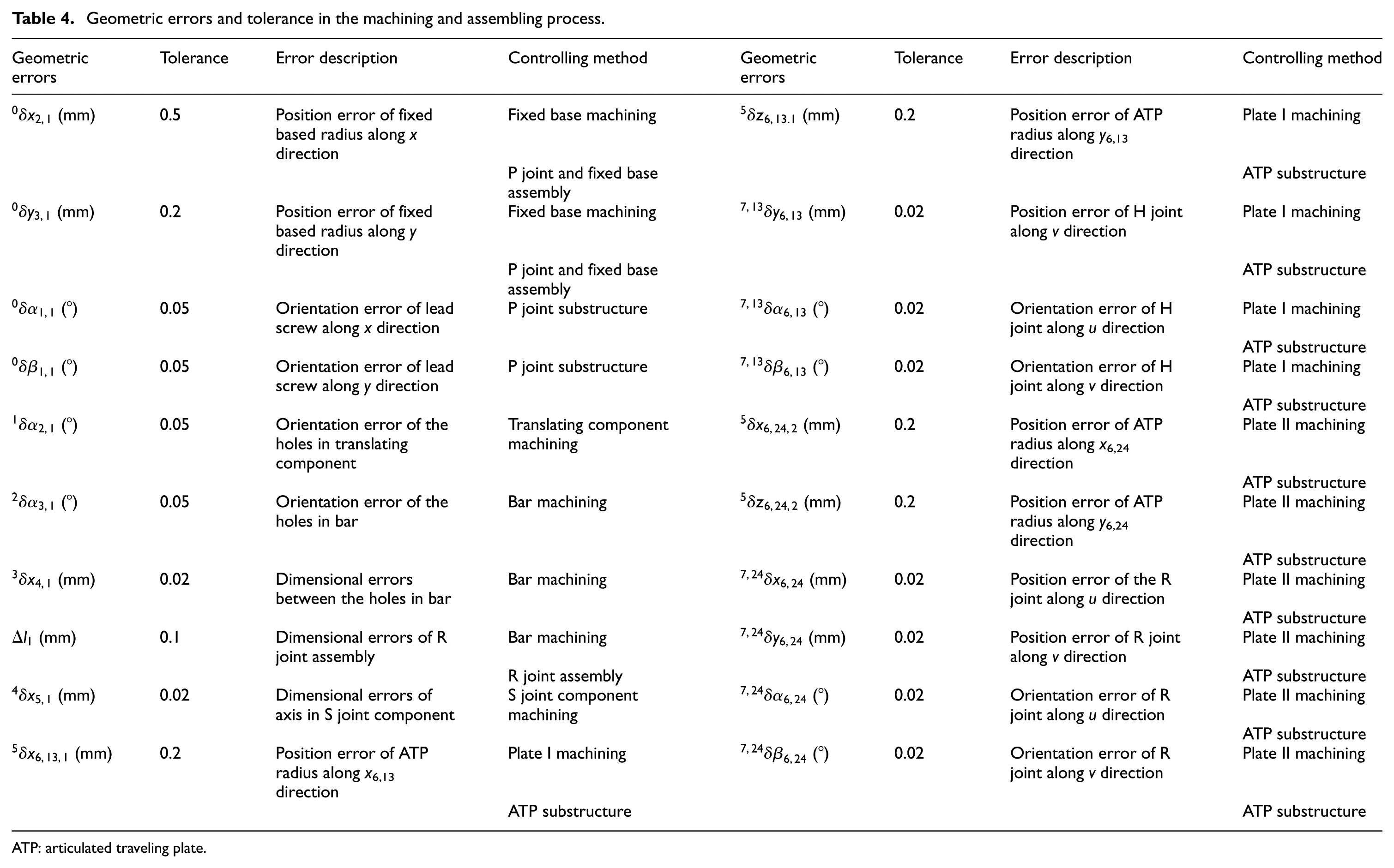
As mentioned above, geometric accuracy design was to restrain geometric errors in component machining and substructure assembling process. According to the composition of PaQuad PM, the concerned components in the machining process were fixed base, sliding saddle, bar, S joint components, in-part 1, and in-part 2. The assembling techniques were mainly for P joint substructure, P joint and fixed base assembly, R joint substructure, R joint and P joint assembly, S joint substructure, and ATP substructure. Corresponding machining/assembling tolerances and the geometric errors are listed in Table 4 in Appendix 3.
Component machining
Corresponding to geometric errors, dimensional and geometric tolerances are divided in the component machining process. Dimensional tolerance describes the position accuracy of component parameters while geometric tolerance shows the orientation accuracy of component features. By setting correct tolerance, the high-precision machining process was capable of restraining geometric errors. Then, measurement of these geometric errors was carried out to provide reference for assembling. Only typical dimensional and geometric errors in the main components are shown below, and the rest of the errors follow the same tolerance setting and measuring principles.
For the fixed base, dimensional tolerance of the distance between opposite board slots was taken into account. It was to assure radius of the fixed base. Geometric tolerance about co-planarity of assembling reference planes was required for orientation accuracy of opposite PRS limbs. The dimensions were measured by coordinate measuring machine (CMM).
For the translating component, axis 1 and axis 2 were collinear with the axis of lead screw and R joint. Geometric tolerance for perpendicularity of axis 1 and axis 2 was the priority, which corresponded to orientation error
For the bar, dimensional tolerance relating to the distance between axis 2 and reference plane was required. Geometric tolerance about perpendicular of axis 2 and axis 3 was asked for orientation error
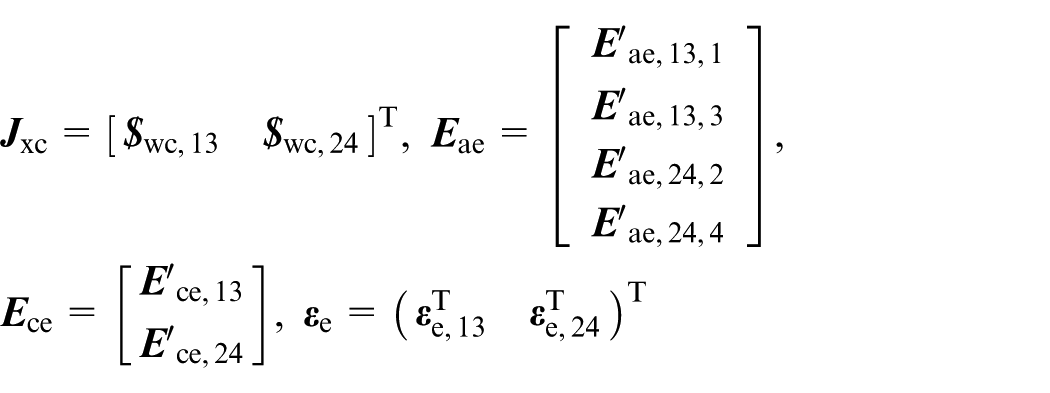
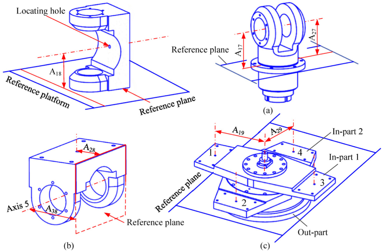
For the S joint components, geometric tolerance about intersections of rotating axis were the main concern, which required axis 3, axis 4, and axis 5 mutually intersecting. The measurement of axis 3 and axis 4 in component 1 is shown in Figure 4(a). The distance between axis 3 and reference plane
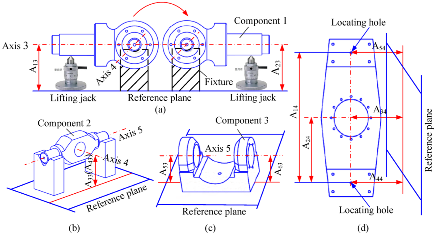
Accuracy design and measuring of the (a–c) S joint components and (d) plate I.
For the ATP, in-part 1 was taken as example to demonstrate the setting of machining tolerance and error measurement. Dimensional tolerance about the length of in-part 1 was restricted, as well as geometric tolerance for co-planarity of locating holes and H joint. Geometric error measurement was as shown in Figure 4(d). The distance between two locating holes
Substructure assembling
Based on the measured component errors, assembling technique is to further eliminate or minimize geometric errors. In general, assembling process can be summarized as (1) regard machining reference plane as assembling reference plane, (2) select several measuring points on the same plane or axis and then measure the distances between measuring points and reference plane, and (3) obtain required tolerance by adjusting components. The main substructures, P joint substructure, P joint and R joint assembly, S joint substructure, and ATP are chosen as example to demonstrate substructure assembling.
For the P joint substructure, translating accuracy was the primary consideration. Therefore, group assembling technique was adopted for the two sets of guide-slider. Installation of lead screw required the same height for bearing pedestals and connecting holes in sliding saddle. Three locations were selected to measure the distances between connecting hole and reference plane
For the P joint and R joint assembly, co-planarity between axis 3 and lead screw axis was the most important, which corresponded to orientation error
For S joint substructure, dimensional tolerance of component 1 was required for determining the length of R joint substructure, which corresponded to position error
Assembling of (a and b) S joint substructure and (c) ATP.
For the ATP, position tolerance about the lengths of in-part 1 and in-part 2 is the most important. Geometric tolerance relating to concentricity of parts was demanded. In-part 2 connected to out-part through bearing (R joint). In-part 1 was fastened to out-part through screw/nut (H joint). The plate length and concentricity was guaranteed by adjusting R joint and H joint as was shown in Figure 5(c).
Error compensation
Identification modeling
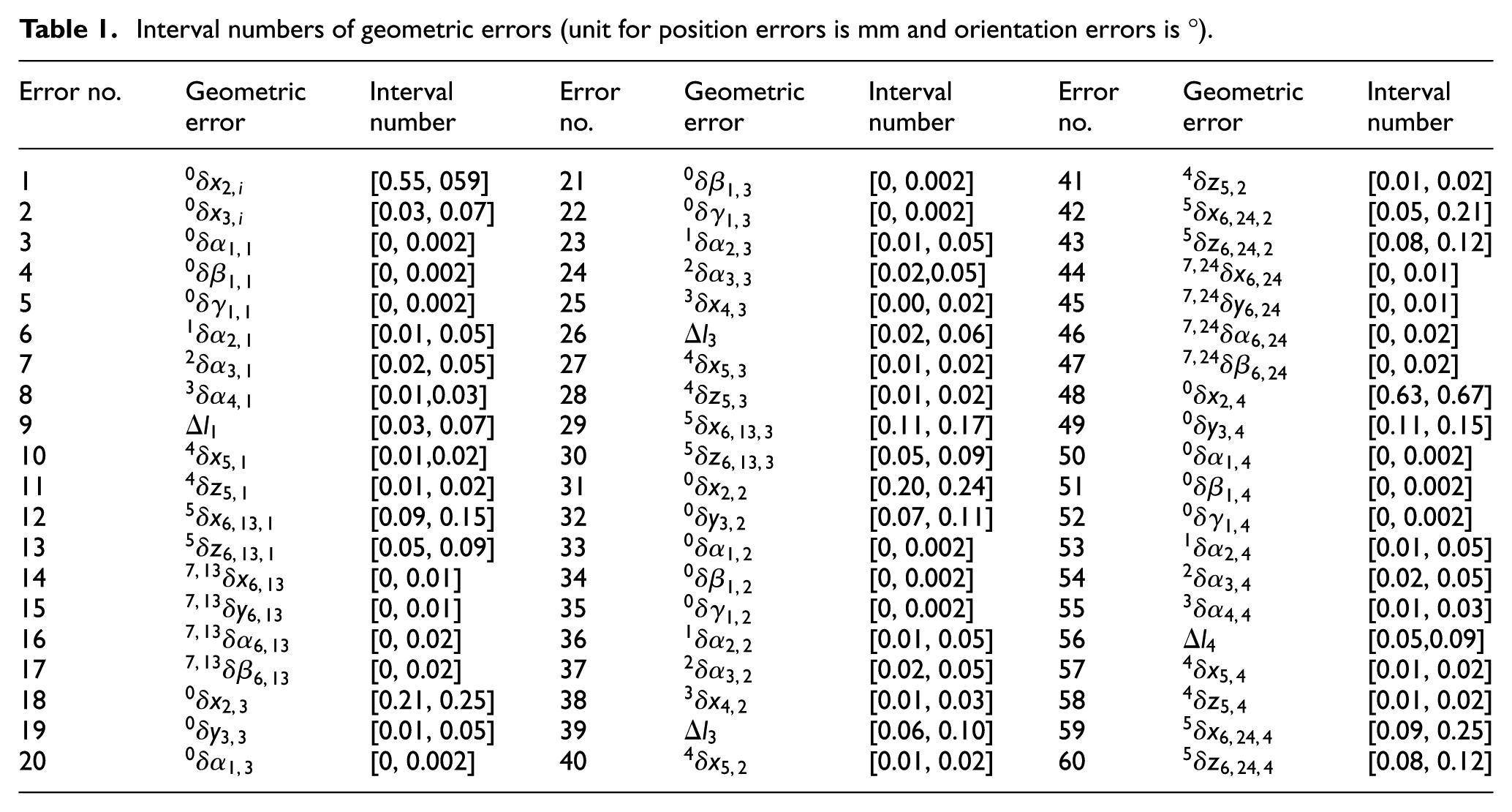
Note that substantial geometric errors would lower the efficiency of kinematic calibration. Sensitivity analysis was carried out to exclude geometric errors that had little effect on the accuracy of PaQuad PM. The range of actual geometric errors was first obtained by error measurement. Considering the uncertainty of measurement, interval number was introduced to describe geometric errors as shown in Table 1. For the convenience of geometric error analysis, the upper and lower limits of geometric errors were shown by their absolute value.
Interval numbers of geometric errors (unit for position errors is mm and orientation errors is °).
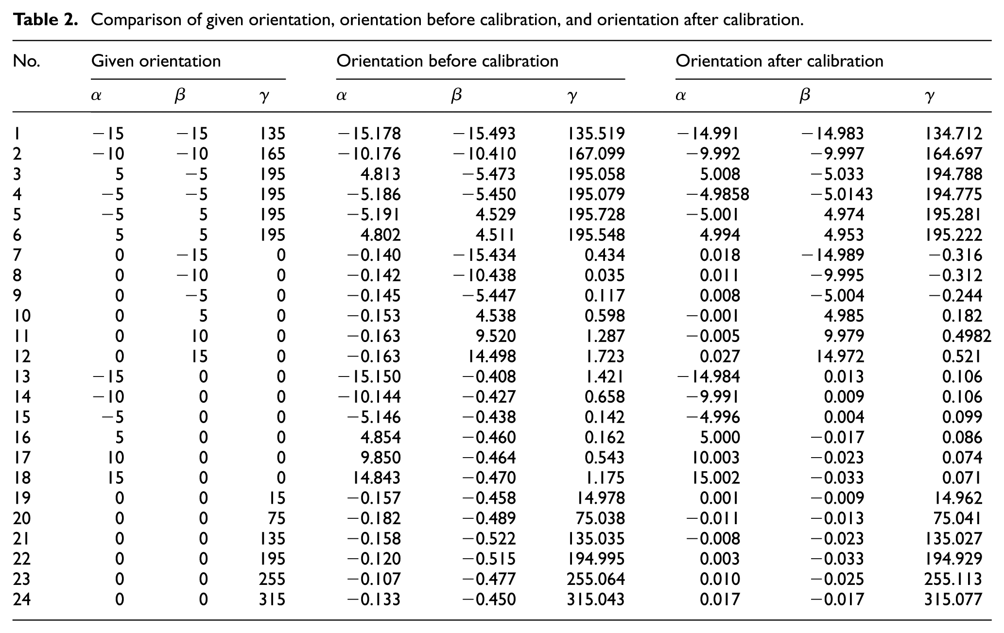
Comparison of given orientation, orientation before calibration, and orientation after calibration.
Referring to geometric error model in equation (7), sensitivity coefficients of geometric errors with respect to errors of PaQuad PM can be expressed as
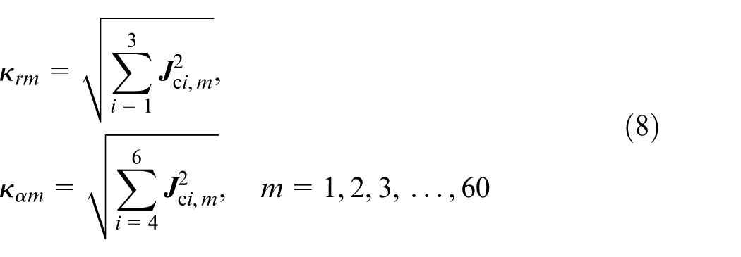
where

By replacing

where
Sensitivity of geometric errors can be obtained by substituting the upper limit into equation (17). The results were shown in Figure 6. It is summarized that No. 5, 35 errors
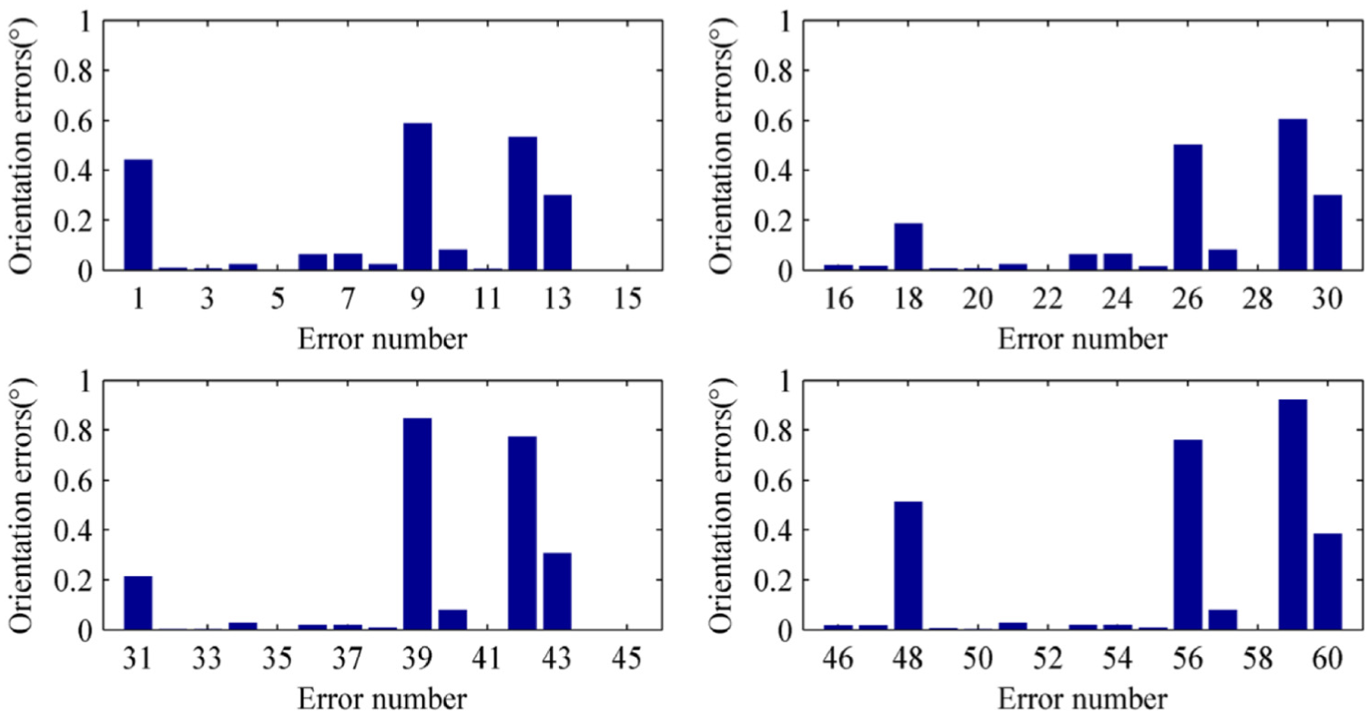
Sensitivity analysis of the geometric errors.
After geometric error sensitivity analysis, identification modeling between geometric errors and measuring data can be implemented. Laser Tracker was adopted as the measuring device, whose measuring reference frame is assigned automatically. Closed-loop equation is formulated as

where
Taking the first-order perturbation on both sides of equation (11) yielded

where
Substituting geometric model in equation (7) into equation (12) yielded

where
herein,
Let

where
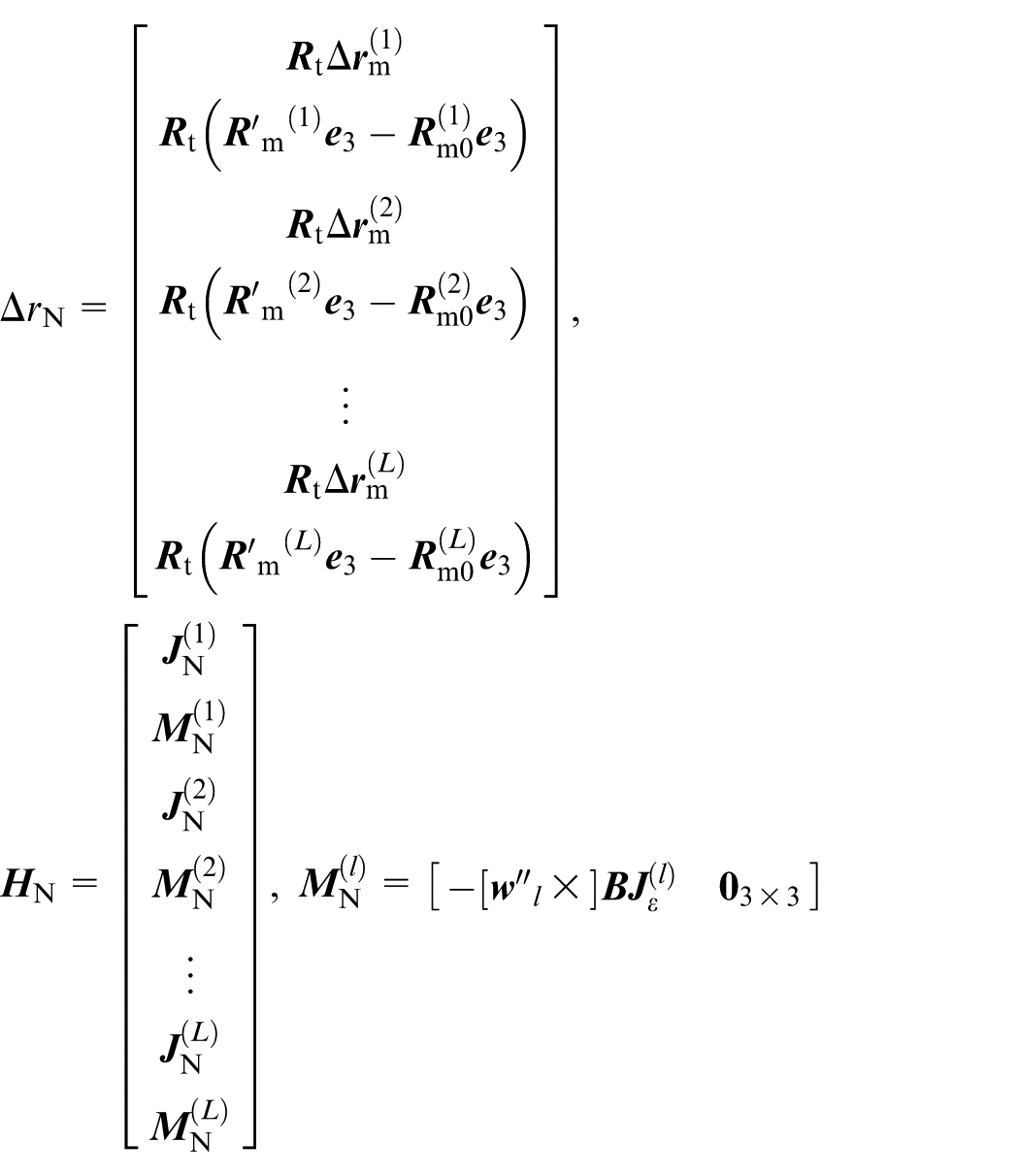
herein,
In order to obtain inverse solution for equation (14), Tikhonov regularization 24 was applied to solve the ill-conditioning problem. Then, identification model can be expressed as
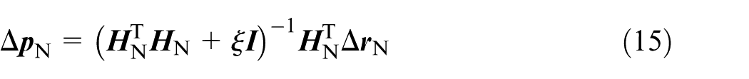
herein,
From equation (14), the relation between
Measurement planning
Measurement planning was to select measuring numbers and configurations. For 1T3R PaQuad PM, translation along z-axis did not affect the identification of geometric errors since it was linear dependent to P joints (see experimental verification in Appendix 2). To identify all geometric errors, PaQuad PM should go through three rotational DoFs at the measuring configurations. Therefore, measuring configurations were determined on a plane with fixed z value. And they are evenly distributed in the orientation workspace
Since singularity of identification matrix
Parameter identification and error compensation
Geometric error identification and compensation was implemented by calibration experiment. This procedure can be summarized as (1) drive PaQuad PM going through all measuring configurations, (2) obtain measuring data through Laser Tracker, (3) identify geometric errors by identification model, and (4) modify geometric errors in the control system. In this process, establishment of fixed frame and selection of reference points were the most important preparations.
The establishment of fixed frame
Selection of reference points should be capable of calculating rotating angles of PaQuad PM. For this purpose, points
The orientation of PaQuad PM can be calculated by coordinates of points
The calibration experiment was set up as shown in Figure 7, in which Laser Tracker with type number Leica-AT901-LR was adopted. With the measurements of points
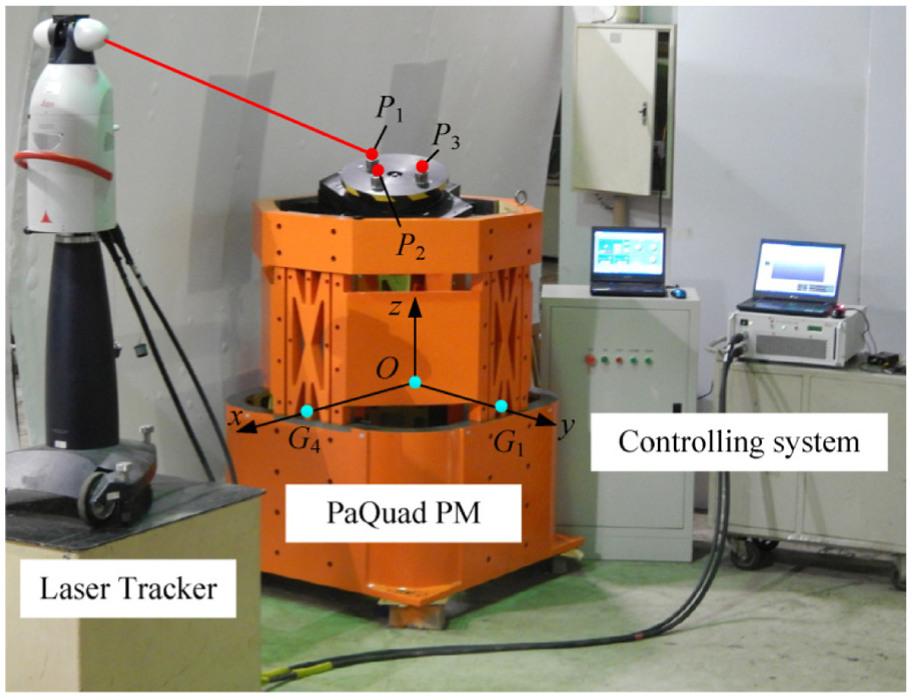
Calibration experiment of PaQuad PM.
Experimental verification
In order to verify accuracy improvement in terms of geometric accuracy design and error compensation, 24 testing points were chosen. These testing points were different from measuring points in kinematic calibration.
Comparison of orientations before and after kinematic calibration was shown in Figure 8. It can be summarized that (1)
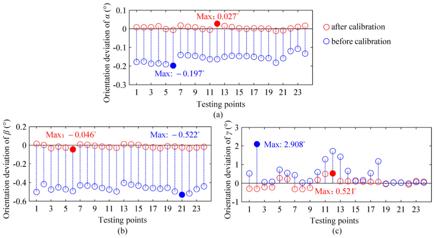
Orientation accuracy of PaQuad PM before and after kinematic calibration (a) deviation of α (b) deviation of β (c) deviation of γ
In Zhong et al.,
43
the assembly accuracy range of aircraft wing skin is (−0.273, +0.350) mm based on contour board. And it becomes (−0.36, +0.25) mm based on coordinate holes. Comparatively, position accuracy of PaQuad PM along z-axis is
Experimental verification and comparison with other docking equipment indicates that error compensation by means of kinematic calibration was effective. Furthermore, it confirms the efficiency and correctness of accuracy improvement strategy proposed in this article.
Conclusion
Focusing on the high-precision assembling of large-scale components in aerospace, shipbuilding, and construction machinery, 1T3R PaQuad PM was taken as an example to investigate accuracy improvement of docking PMs. It was carried out by geometric error modeling, geometric error design, and error compensation. Corresponding conclusions are drawn as follows:
Based on screw theory, geometric error modeling of PaQuad PM was obtained from four independent routes. Each route error twist was formulated by superposition of geometric errors and joint perturbations. Single wrench within each route and combination wrench provided by opposite routes were applied to eliminate joint perturbation.
Geometric accuracy design restrained geometric errors at component and substructure levels. Geometric errors were first transferred into dimensional or geometric tolerance. High-precision machining and assembling techniques were then adopted to satisfy the tolerances. Error measurement was finally implemented to provide reference for kinematic calibration.
Error compensation was conducted by kinematic calibration at mechanism level. Sensitivity analysis by means of interval theory was applied to exclude unimportant geometric errors. L-curve selection was employed to solve ill-conditioning problem in the identification modeling. In all, 48 evenly distributed measuring configurations were determined by taking both efficiency and accuracy into account.
Maximum deviations of PaQuad PM before calibration experiment was 0.01 mm,
Footnotes
Appendix 1
Appendix 2
In order to prove the high accuracy of PaQuad PM along z direction, calibration experiment is carried out as:
The error of the distance between two planes is 0.01 mm, which proves that the accuracy of PaQuad PM along z direction before error compensation is acceptable. The change of z value does not affect geometric error identification.
Appendix 3
Geometric errors and tolerance in the machining and assembling process.
| Geometric errors | Tolerance | Error description | Controlling method | Geometric errors | Tolerance | Error description | Controlling method |
|---|---|---|---|---|---|---|---|
| 0.5 | Position error of fixed based radius along x direction | Fixed base machining | 0.2 | Position error of ATP radius along y6,13 direction | Plate I machining | ||
| P joint and fixed base assembly | ATP substructure | ||||||
|
|
0.2 | Position error of fixed based radius along y direction | Fixed base machining |
|
0.02 | Position error of H joint along v direction | Plate I machining |
| P joint and fixed base assembly | ATP substructure | ||||||
|
|
0.05 | Orientation error of lead screw along x direction | P joint substructure |
|
0.02 | Orientation error of H joint along u direction | Plate I machining |
| ATP substructure | |||||||
|
|
0.05 | Orientation error of lead screw along y direction | P joint substructure |
|
0.02 | Orientation error of H joint along v direction | Plate I machining |
| ATP substructure | |||||||
|
|
0.05 | Orientation error of the holes in translating component | Translating component machining |
|
0.2 | Position error of ATP radius along x6,24 direction | Plate II machining |
| ATP substructure | |||||||
|
|
0.05 | Orientation error of the holes in bar | Bar machining |
|
0.2 | Position error of ATP radius along y6,24 direction | Plate II machining |
| ATP substructure | |||||||
|
|
0.02 | Dimensional errors between the holes in bar | Bar machining |
|
0.02 | Position error of the R joint along u direction | Plate II machining |
| ATP substructure | |||||||
|
|
0.1 | Dimensional errors of R joint assembly | Bar machining |
|
0.02 | Position error of R joint along v direction | Plate II machining |
| R joint assembly | ATP substructure | ||||||
|
|
0.02 | Dimensional errors of axis in S joint component | S joint component machining |
|
0.02 | Orientation error of R joint along u direction | Plate II machining |
| ATP substructure | |||||||
|
|
0.2 | Position error of ATP radius along x6,13 direction | Plate I machining |
|
0.02 | Orientation error of R joint along v direction | Plate II machining |
| ATP substructure | ATP substructure |
ATP: articulated traveling plate.
Declaration of conflicting interests
The author(s) declared no potential conflicts of interest with respect to the research, authorship, and/or publication of this article.
Funding
The author(s) disclosed receipt of the following financial support for the research, authorship, and/or publication of this article: This research work was supported by National Natural Science Foundation of China (NSFC) under Grant Nos 51475321, 51305293, and 51205278 and Tianjin Research Program of Application Foundation and Advanced Technology under Grant No. 15JCZDJC38900.