
Abstract
A three-point method based on sequential multilateration is applied to measuring the geometric error components (GECs) of three-axis machine tools (MTs). To meet the accuracy requirement of geometric error mapping, a sequential multilateration scheme is developed for high-accuracy point measurement by introducing four additional targets into the measuring system, and the uncertainty of point measurement is verified by simulation. Three independent targets fixed on the MT’s spindle assembly move along with each axis step by step and their coordinates at each step can be determined by the distance data acquired by laser tracker at all steps based on sequential multilateration. Then the volumetric errors of the three target points can be obtained by comparing the actual coordinates and the corresponding desired coordinates, and nine equations can be established by substituting volumetric errors into the error model of linear axis, so that the six GECs of each axis can be obtained by solving these equations. The three squareness errors can be determined by computing the angles between the average lines of the three axes which are achieved by linear curve fitting. Experiments are conducted to measure these 21 GECs, and the volumetric errors in the three-axis MT’s workspace, which are determined by these measured GECs based on the error model of three-axis MT, are compensated. Finally, the positioning errors of the MT with compensation and without compensation are evaluated by laser interferometer, respectively, the experimental results of which demonstrate that the positioning errors are significantly reduced by the error compensation.
Keywords
Introduction
Accuracy is one of the most crucial considerations for evaluating machine tools. The machine tool errors which can be mainly classified into quasi-static errors and dynamic errors have direct influence on the accuracy of machine tools. The quasi-static errors are those between the tool and the workpiece that are infinitely slowly varying with time and related to the structure of the machine tool itself, and they account for about 70% of the total machine tool errors. 1 The geometric errors are the key contributors to the overall quasi-static errors of machine tools, so that many researchers have been dedicated to the research of geometric error measurement and compensation. Generally, accuracy enhancement by using error compensation can be divided into three steps: measuring errors, establishing error model and compensating errors. 2 Therefore, as the basis of the geometric error compensation, measurement of geometric error has been a hot topic, and many researchers focused on the development of effective methods for measuring the geometric error components of machine tools with high accuracy.
For three-axis machine tools, there totally exist 21 geometric error components. Researchers have proposed many methods based on laser interferometer to measure these geometric error components. Many displacement-measurement-based methods have been developed to measure all the 21 geometric error components by locating points along 22 lines, 15 lines, 14 lines and 9 lines within the workspace of the three-axis machine tools.3–6 Charles Wang 7 proposed a laser vector measurement technique to determine all the 21 geometric error components by measuring the positioning errors along four body diagonals in the workspace of machine tools. Mark A.V. Chapman 8 pointed out that the laser diagonal measurement is not reliable for assessing the volumetric errors, and the step diagonal method is not reliable for evaluating linear errors. The recommendations were proposed to validate the error mapping, which also provided guidance for the practical application. Another powerful device, the 6D laser interferometer can detect all the six geometric error components of linear axis and rotary axis with prismatic joint, 6D sensors and other accessories. 9 These laser-interferometer-based approaches mentioned above can measure the geometric error components with high accuracy. However, due to the utilization of the laser interferometer, these methods always require complicated installation procedure and experienced operator. Furthermore, the measurement on each axis or each line has to be accomplished in turn, which leads to considerable amount of measurement time and unavoidable error induced by repeating the installation of measuring equipment.
There are also many methods for measuring geometric error components of machine tools without laser interferometer. Double ball bar (DBB) which is proposed by Bryan in 1982 has been applied to evaluate and check the accuracy of multi-axis machine tools.10–13 The DBB-based methods are economical and particularly simple to acquire data. However, due to the size of DBB, it always cannot cover the whole workspace of machine tools, especially for the large machine tools. Lee et al. 14 have developed a multi-degree-of-freedom measurement system to identify the geometric error components of miniaturized machine tools by using five capacitance sensors, a fixture and a target. This system is of low cost and can be used relatively simply. However, it is not suitable for geometric error measurement of different-sized machine tools due to the size of accessories; furthermore, this method is incapable of measuring the positioning error. Gao et al. 15 developed a three-axis autocollimator system with excellent accuracy, although it can only measure the angular error of linear axis. An instrument consisting of three rotary encoders and link mechanisms has been developed to measure positioning errors on arbitrary tool paths in the workspace of machine tool; 16 it is of low cost, but the measuring range is limited by the size of link mechanisms. Cross-grid encoder is a precise device for two-dimensional (2D) position measurements, and many researchers have developed several methods for accurate geometric error measurement of machine tools.17,18 The measuring range of these methods is limited by the size of grid encoder, so that it is not suitable for geometric errors measurement of long-range machine tools.
The laser tracker (LT) is a three-dimensional measurement instrument in large-scale metrology. Researchers developed several methods for identifying geometric error of machine tools by using LT. Umetsu et al. 19 used multilateration method to realize a high-accuracy three-dimensional (3D) coordinate collection, and the geometric error components of machine tools can be obtained by allocating the measured points on 21 lines in the six planes of the measurement volume by using the multilateration principle. However, this method is of high cost since four LTs are involved, and the measurement is conducted on up to 21 lines, so it is time-consuming. Aguado et al.20,21 proposed a strategy for identifying the parameters in volumetric error compensation of machine tools by using three LTs. This strategy measures a set of points which discretize the workspace of the machine tool, and then, regression analysis is applied to characterize the geometric error parameters. The measurements for numerous sample nodes may lead to a large amount of measuring times. Wang et al. 22 made use of a sequential multilateration method which requires only one LT to calibrate the numerical control (NC) machine tools, and the cost is greatly reduced. The LT is located at four different stations of which the positions can be determined by the nominal positions of the under-test points based on multilateration principle, and then, the actual coordinates of the under-test points can be determined by the identified coordinates of the LT’s stations based on the multilateration principle. But as the volumetric errors of under-test points will contribute to the overall uncertainty of the base-stations’ self-calibration, it is hard to guarantee that the c-coordinates of the under-test points on the four lines will be same to each other when identifying the geometric errors of c-axis (c denotes x, y or z) at each step, the under-test points’ coordinate and the geometric error components are obtained by using iterative computations, which lead to a long calibration time. Another sequential multilateration method has been applied to measure coordinates of target points by locating only one LT at four stations in turn. 23 The mathematical model of this sequential multilateration method is identical with the multilateration principle, and it is applicable to measuring the coordinates of a set of fixed points with high accuracy. But its accuracy is unsatisfactory for measuring the points which have repeatability, such as measuring the sample points when calibrating machine tools, because the repeatability of the under-test points will contribute to the overall uncertainty of the systematic self-calibration.
To overcome the shortcoming of methods mentioned above, a three-point method for measuring the geometric errors of three-axis machine tools is presented in this article. The authors have used this method to measure geometric error components of a single linear axis. 24 In this article, further work is done. By using three-point method, all the 21 geometric error components of three-axis machine tools can be easily obtained by measuring the coordinates of three points with a single LT, and furthermore, the accuracy of coordinate measurement is improved by using sequential multilateration scheme. The number of sample nodes is small, so the measurements are time-saving. Due to no requirement of complicated installation and alignment, this method is simple and fast, and no experienced operator is necessitated. The rest of this article is organized as follows: in section “Error model of three-axis machine tool,” the error model of linear axis and three-axis machine tools which can explicitly describe the relationship between the volumetric error and the geometric error components is introduced. In section “Coordinates collection by using LT,” a sequential multilateration method based on a LT is presented for the accurate 3D coordinate measurement. In section “Method for geometric error measurement,” a three-point method is presented to measure the six geometric error components of linear axis and the squareness errors between the three axes of machine tool by collecting the 3D coordinates of three given points when they move along three axes within the machine workspace. In section “Experiments and analysis,” the volumetric errors are obtained by using the error model of three-axis machine tools, and the experiments are conducted to validate the effectiveness of the presented method. Finally, the conclusion and summary are addressed in section “Conclusion.”
Error model of three-axis machine tool
Error model of linear axis
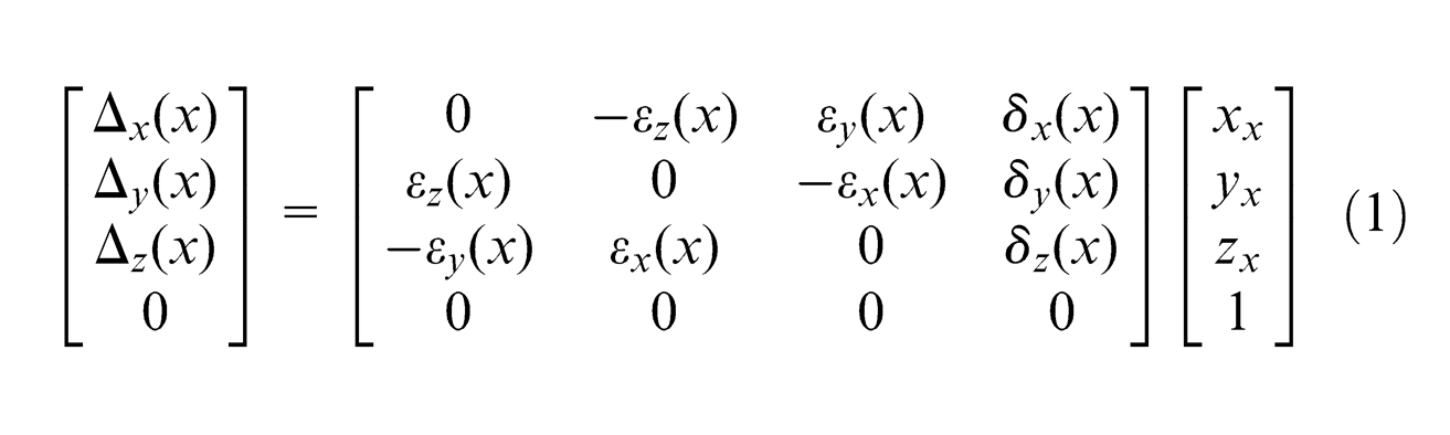
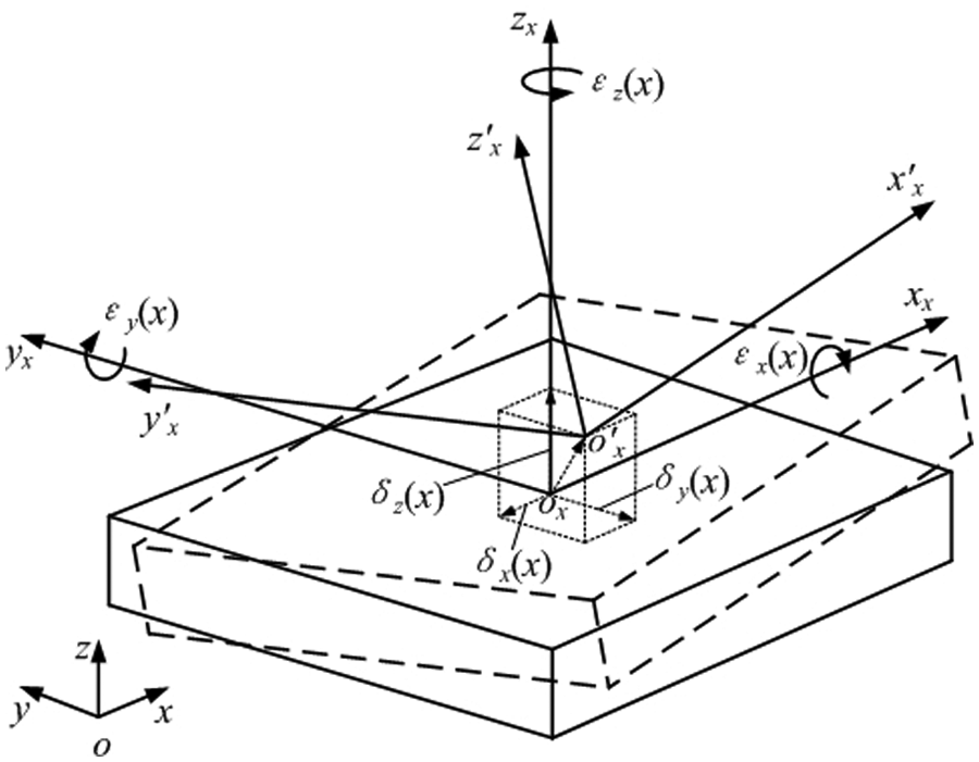
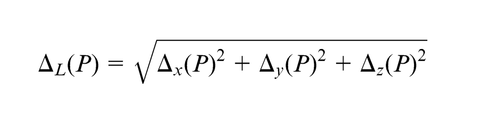
As shown in Figure 1, oxyz, oxxxyxzx and o′xx′xy′xz′ x are the reference coordinate frame (RCF), nominal x-slide coordinate frame and the actual x-slide coordinate frame, respectively. The pose of actual x-slide coordinate frame varies because of the six geometric error components and the displacement x. The 4 × 4 homogeneous transform matrix (HTM) can be used to characterize the relationship between the RCF and the actual coordinate frame of x-slide. The volumetric errors can be obtained by equation (1) 1
Geometric error components of linear axis.
where Δ x (x), Δ y (x) and Δ z (x) are the three volumetric error components, [xx, yx, zx, 1]T is the homogeneous coordinates of the measured point in the x-slide coordinate frame, δx(x) is the positioning error, δy(x) and δz(x) are the two straightness errors, εx(x) is roll error, εy(x) is pitch error, εz(x) is yaw error and the x in the round brackets is the displacement of x-slide.
Error model of three-axis machine tool
Each linear axis of three-axis machine tool has six geometric error components. There also exist three squareness errors caused by nonorthogonality between the three axes. Thus, there are totally 21 geometric error components of three-axis machine tool. The error model of three-axis machine tool can be derived by 4 × 4 HTM and rigid body kinematics. The positioning error of three-axis machine tool is considered as the deviation between the actual tool position and the desired tool position. The actual tool position can be obtained by multiplying all the HTMs with error components successively starting from the RCF to the tool coordinate frame; similarly, the desired tool position can be obtained by multiplying all the HTMs without error components successively starting from the RCF to the tool coordinate frame.
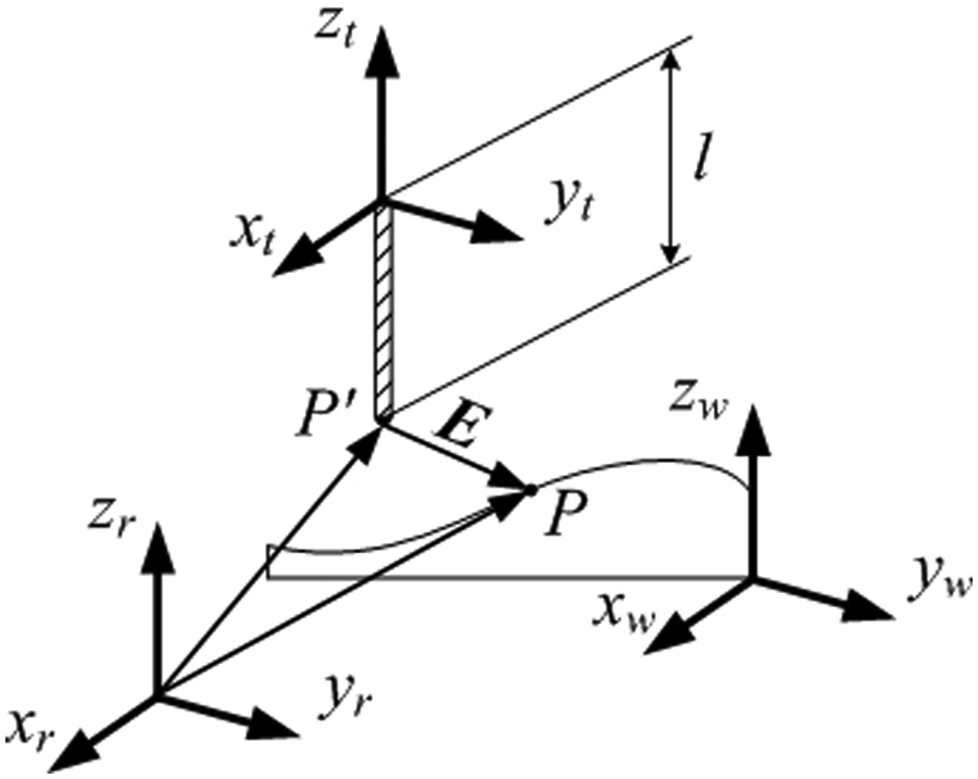
Usually, three-axis machine tools can be classified into four types, that is, FXYZ, XFYZ, XYFZ and XYZF, and in the name of each type, the letters before F denote the available motion directions of the workpiece, and the letters after F denote the available motion directions of the tool. Take type FXYZ as an example, the schematic diagram of the structure of three-axis machine tool and six corresponding coordinate frames, that is, RCF orxryrzr, x-slide coordinate frame oxxxyxzx, y-slide coordinate frame oyxyyyzy, z-slide coordinate frame ozxzyzzz, tool holder coordinate frame ohxhyhzh and workpiece coordinate frame owxwywzw are illustrated in Figure 2.
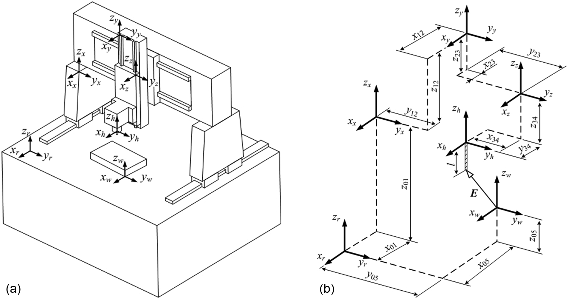
Coordinate frames of three-axis machine tools: (a) the sketch map of three-axis machine tool and (b) the coordinate frames.
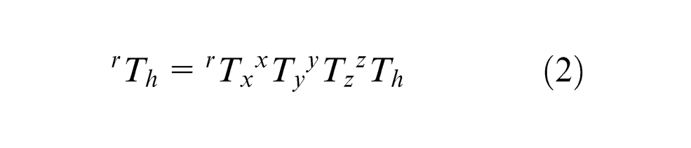
The homogeneous transformation matrix that can describe the spatial relationship between the RCF and the tool coordinate frame can be given as 1
where
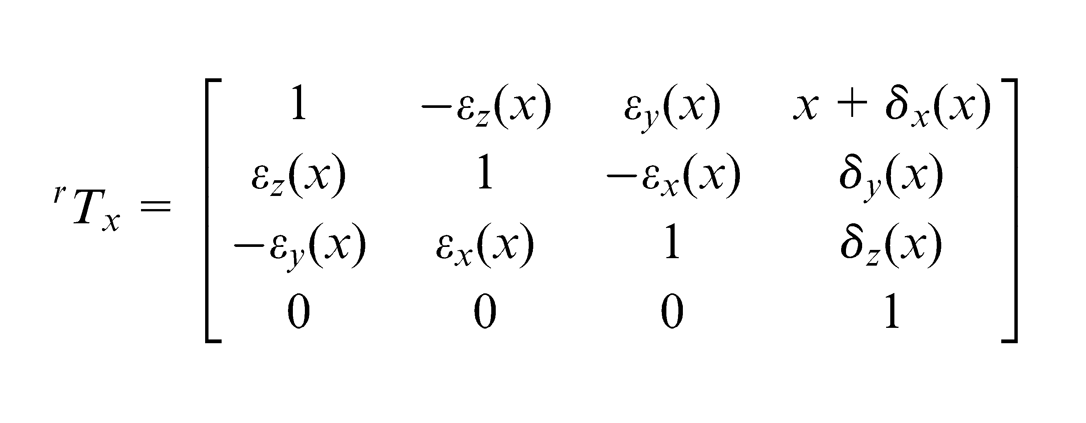
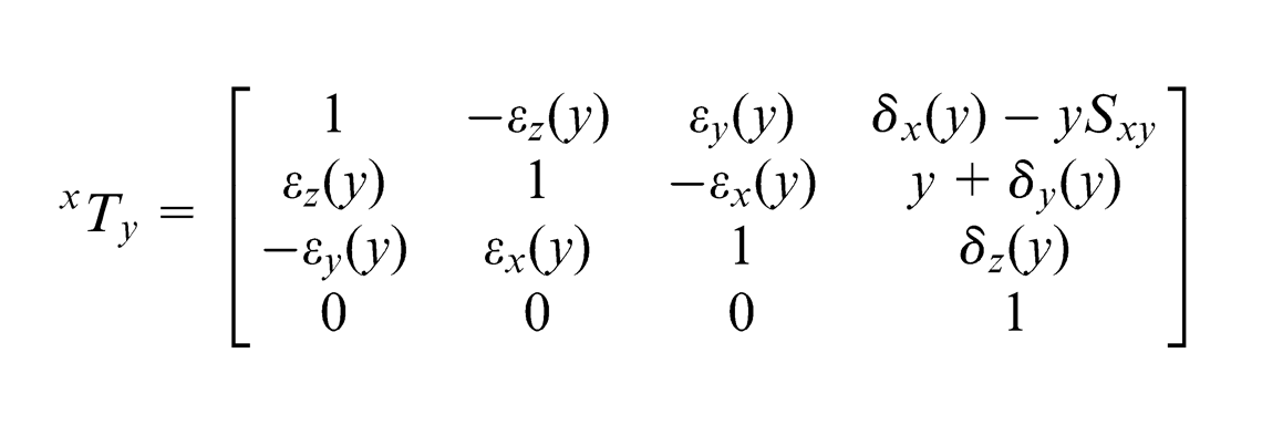
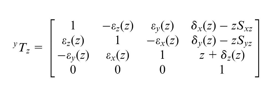
where δi(j) (i, j = x, y, z) are the positioning errors (if i = j) or straightness errors (if i≠j) in the direction of i-axis when the j-axis moves, εi(j) (i, j = x, y, z) are angular errors about i-axis when the j-axis moves and Sij are the squareness errors between axis i and j.
For convenience, the offsets (y01, z12, x12, x34, y34 etc. as shown in Figure 2, between the coordinate frames of adjacent axes are set to zero in initial status, that is to say, all the origins of coordinate frames are in coincidence with each other in initial status. In matrix
So the actual coordinates of tool tip
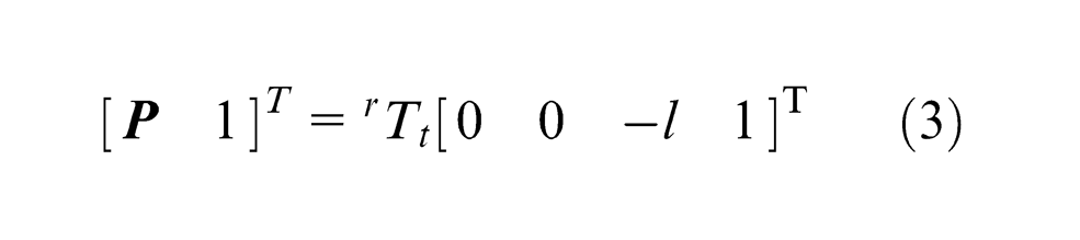
where l is the length of tool.
And the desired coordinates of tool tip in the RCF,
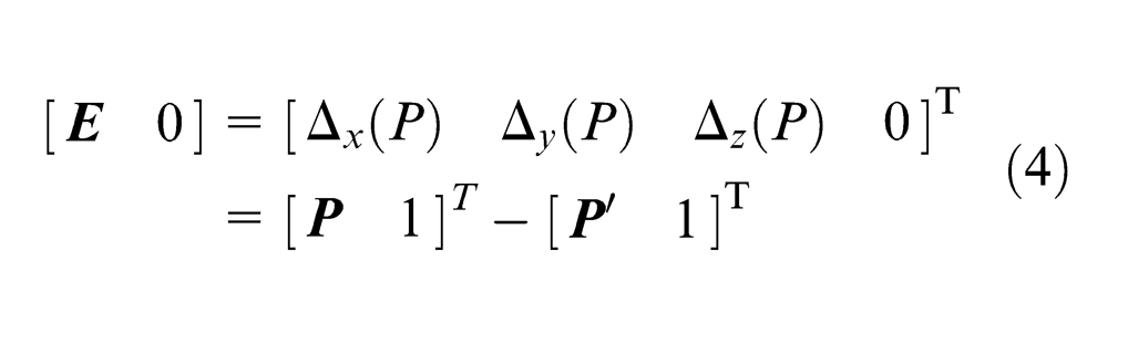
The higher order infinitesimal terms (no less than 2) are neglected in the final results, so concretely, the volumetric error components are
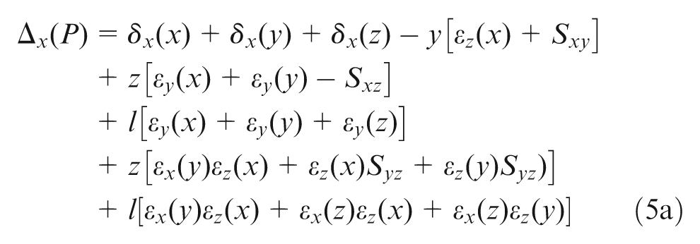
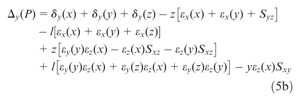
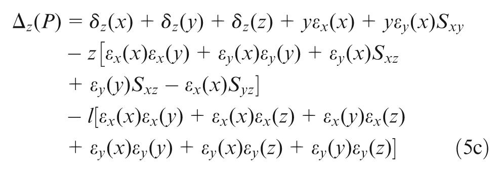
where x, y and z in the parentheses are the displacements of the x-slide, y-slide and z-slide, respectively.
The volumetric error vector is shown in Figure 3, and the length of the volumetric error vector can be computed by
Volumetric error vector of machine tool.
Coordinates collection by using LT
A sequential multilateration method
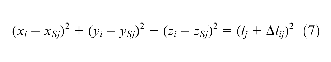
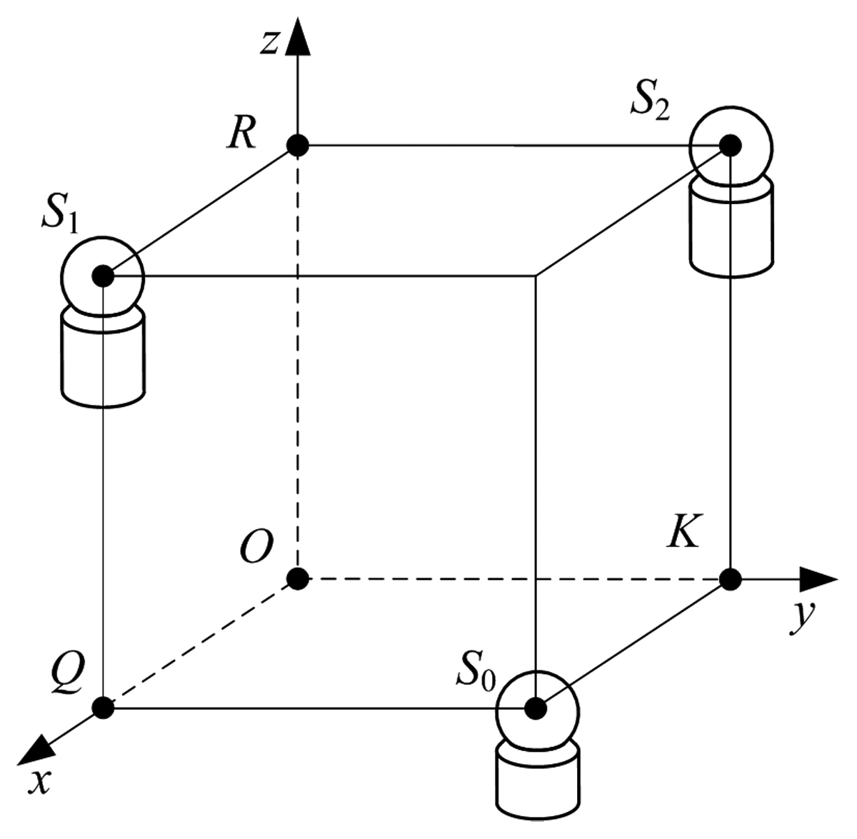
In this article, a sequential multilateration method is developed to detect 3D coordinates. The proposed measuring system is made up of a LT and four additional targets O, Q, K and R, as shown in Figure 4. We assume that the relative positions of these four targets together with other six targets have been determined by sequential multilateration principle. 23 The RCF is established as follows: let point O be the origin of RCF, let the x-axis pass through point Q and the x–y coordinate plane pass through point K. The directions of three axes obey the right-hand rule. The coordinates of O, Q and K are (0, 0, 0), (xQ, 0, 0) and (xK, yK, 0), respectively. Because the incremental length measurement accuracy of the interferometer embedded in the LT is much better than the absolute length measurement accuracy, the incremental length measurement is preferred. So the fourth point R(xR, yR, zR) is defined as a reference point which can provide a reference absolute distance (RAD) between R and LT. The points Pi(xi, yi, zi) (i = 1, 2, 3, …, n) are to be measured.
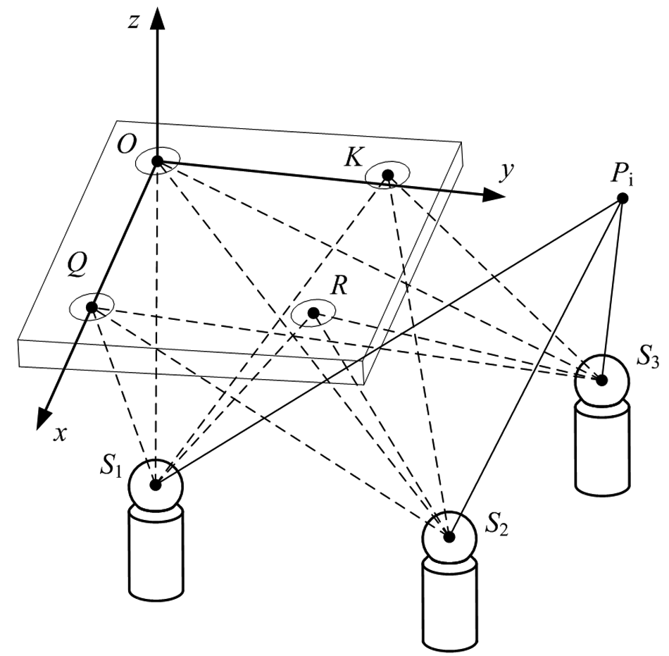
Schematic diagram of the sequential multilateration principle.
The LT is fixed on position Sj(xSj, ySj, zSj) (j = 1, 2, 3). Then, place the retroreflector at R and set the reading of LT to zero. Now define lj, the distance between the Sj and R to be RAD. Then ΔlOj, ΔlQj, ΔlKj and lij, the incremental distances between Sj and O, Q, K, Pi(i = 1, 2, …, n) can be accurately measured by LT, respectively. By using the distance formula between two points, equations (6) and (7) can be obtained
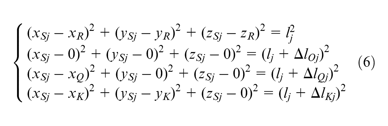
Numerical methods, such as Gradient method, can be used to solve equation (6). (xSj, ySj, zSj) and lj can be obtained by solving equation (6).
Until now, the measurement when fixing the LT on Sj is finished. Though (xSj, ySj, zSj) is known already, (xi, yi, zi) cannot be obtained because there is only one equation (equation (7)) established for point Pi(xi, yi, zi) (i = 1, 2, 3, …, n).
We can repeat the procedure mentioned above three times by locating the LT at three different stations Sj(j = 1, 2, 3). Then, for a certain point Pi(xi, yi, zi), a simultaneous equation which is made up of the three equations (equation (7)) (j = 1, 2, 3) is established
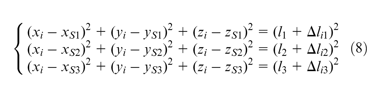
The coordinates of point Pi(xi, yi, zi) can be obtained by solving equation (8).
Pre-determination of the positions of additional targets
The coordinates of the four additional targets should be pre-determined before they are available for the measuring system. We use the sequential multilateration principle as mentioned in literature 23 to determine the relative coordinates of the four additional targets. The self-calibration errors which are induced by repeatability of measured points’ positions are greatly reduced, because the 10 targets are fixed already.
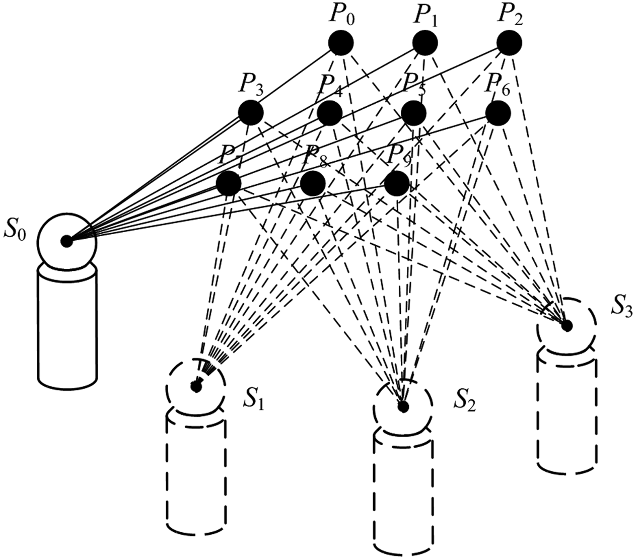
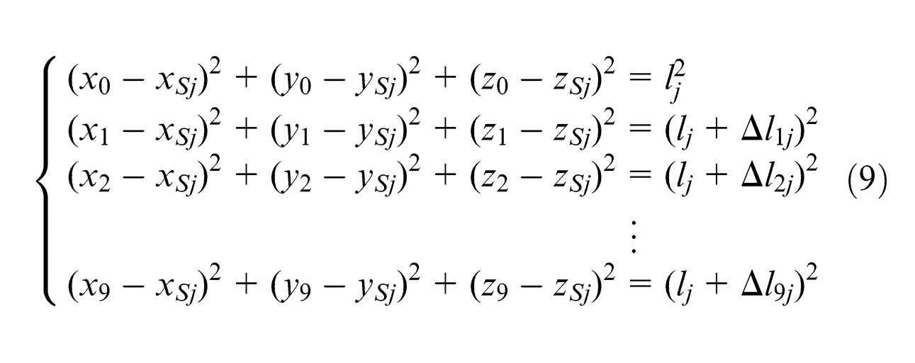
As shown in Figure 5, the four additional targets together with other six target caves, totally 10 targets, are included into the pre-determination procedure. The LT is fixed on four positions Sj(xSj, ySj, zSj) (j = 0, 1, 2, 3) in turn. A RCF, oxyz is established, that is, let the origin locate at S0, let the x-axis pass through S2, let the x–y coordinate plane pass S0. The 3D coordinates of S0, S1, S2 and S3 are (0, 0, 0), (xS1, yS1, 0), (xS2, 0, 0) and (xS3, yS3, zS3), respectively, that is, xS0 = 0, yS0 = 0, zS0 = 0, zS1 = 0, yS2 = 0 and zS2 = 0.
Determination of the positions of additional targets.
The LT is fixed on a certain Sj. P0(x0, y0, z0) is considered as the reference point, the RAD is lj. The incremental distances between LT and the targets Pi(xi, yi, zi) (i = 1, 2, …, 9), Δlij can be measured by LT. Then, we have
There are 10 equations in equation (9). Hence, totally 40 equations can be established after all the four-station measurements are completed, and there are totally 40 unknowns too. Thus, the coordinates of all the targets, including the four additional targets, can be obtained by solving these equations.
Simulations
First, the incremental length measurement accuracy of the LT is verified. Following the method in literature, 19 the verification is realized by comparing the LT with a high-precision reference coordinate measuring machine (CMM) of which maximum permissible error, according to the manufacturer’s catalog, is (0.9 + L/333) µm. Eight target points are arranged to form a circle with diameter being 300 mm. The distances between these points and the LT are approximately 1 m. The nominal coordinates of each target points can be provided by the reference CMM. The self-calibration based on multilateration is applied to obtain the coordinates of LT’s position and the distances between all the target points and the LT. Then, the errors of the distance measurement results can be obtained by comparing the distance values measured by LT and the distance values calculated by the distance formula. This experiment is repeated 20 times, and the maximum deviation and the repeatability are found to be 0.807 and 0.334 µm, respectively.
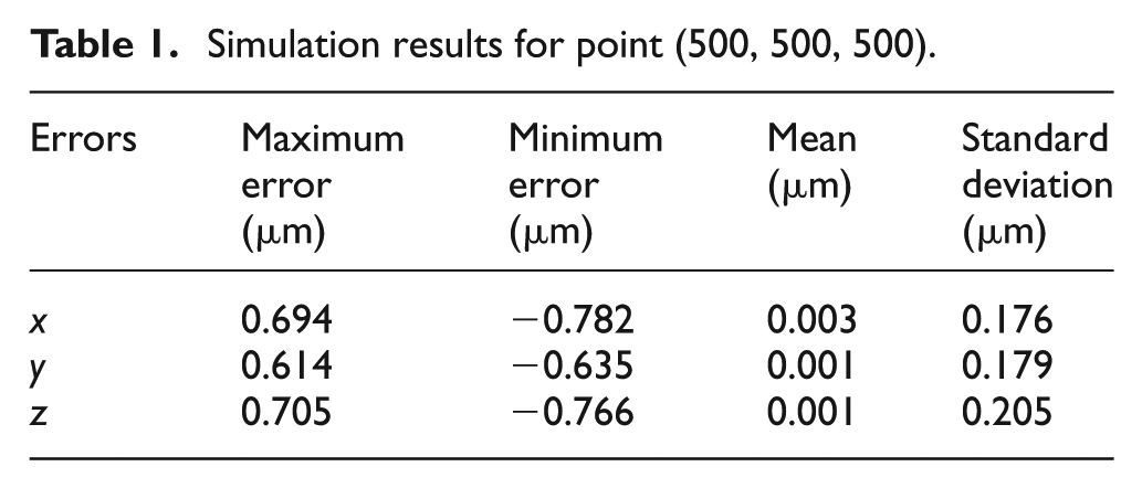
Then, the computer simulation technique is applied to investigate the performance of this measuring system. The first simulation is conducted to estimate the uncertainty of the coordinates of additional targets. The uncertainty of the incremental distance measurement is the only contributor to the uncertainty of measurement, so that a normal distribution is assigned to the incremental distances. According to the 3σ criterion, the repeatability is set as 0.269 µm because the incremental length measurement error of the LT is less than 0.807 µm. Gradient method is used to solve equation (9). The number of simulation trials is 10,000. The simulation results indicate that the maximum deviation is 1.440 µm, and the repeatability is 0.407 µm. The second simulation is conducted to estimate the uncertainty of measurement of the under-test points. There are two contributors to the overall uncertainty of measurement. Because the maximum deviation of the coordinates of additional targets is 1.440 µm, a normal distribution is assigned to the coordinates of additional targets with expectation being zero and standard deviation being 0.480 µm in accordance with the 3σ criterion. The incremental lengths measurement error still has a normal distribution with expectation being zero and standard deviation being 0.269 µm. Gradient method is applied to solve equations (6) and (8). An arrangement of the measuring system is shown in Figure 6. The additional targets and the three stations of LT are located at the apices of the cube which covers the measurement volume. The side length of the cube is 1000 mm, and the number of simulation trials is 10,000. The probability density distribution of measuring error of point Pi(500, 500, 500) is shown in Figure 7, and the detailed results are tabulated in Table 1. A summary of the uncertainty of measurement for the under-test points in the measurement volume is shown in Table 2.
System arrangement of the sequential multilateration principle.
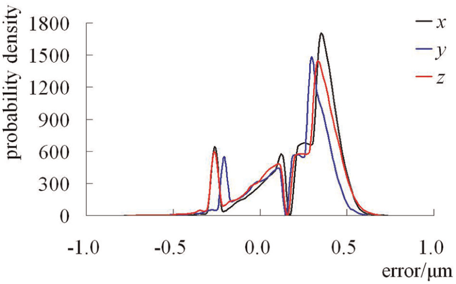
Probability densities of measurement errors of point (500, 500, 500) obtained by simulation.
Simulation results for point (500, 500, 500).
The summary of simulation results.
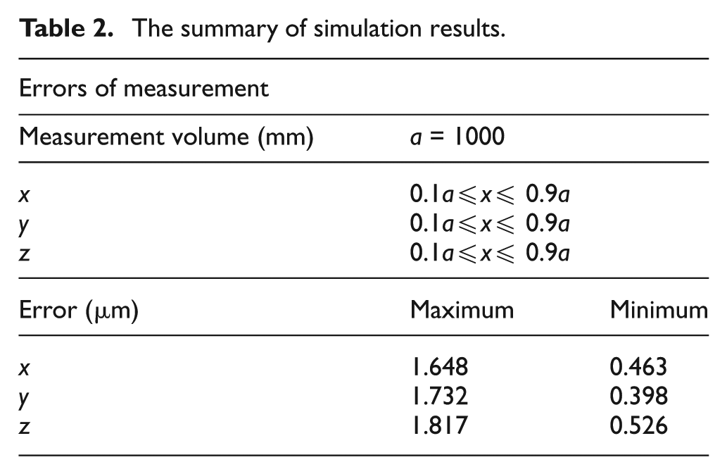
The authors have conducted series of simulations, which presented several conclusions. (1) The arrangement shown in Figure 6 is an optimal arrangement. (2) The probability density distributions of the measuring errors at arbitrary points in the measurement volume are similar to the curve shown in the Figure 7, but the margins of measurement error of the points are different from each other. (3) The maximum errors always occur at the points near the side face of the cube, and the minimum errors always occur at the points near the center point of the cube.
Method for geometric error measurement
Error measurement for linear axis
As shown in Figure 8, x-slide is tested as an example to demonstrate the method for measuring geometric error components of linear axis. Three pre-described points, A, B and C are fixed on the stage of x-slide, and their coordinates are (xxA, yxA, zxA), (xxB, yxB, zxB) and (xxC, yxC, zxC), respectively. oxyz is the RCF, and oxxxyxzx is the x-axis coordinate frame. The six geometric error components of x-slide have been shown in Figure 1, so they are not illustrated in Figure 8.
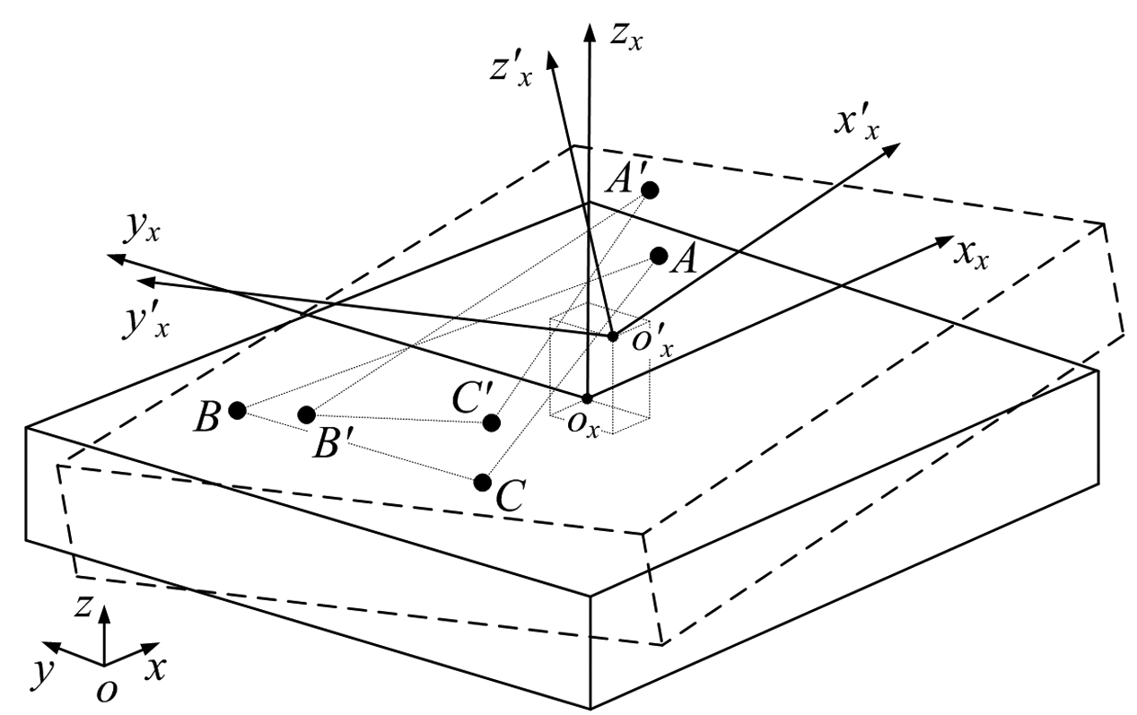
Geometric error measurement of x-slide.
The stage of x-axis moves step by step. At the tth step, the displacement of x-slide is x, and consequently, the volumetric errors at point A are Δ x (A), Δ y (A) and Δ z (A), which can be obtained by using
where (x
where (xO0, yO0, zO0)T is the coordinates of Ox in the RCF when the x-axis locates at the home position.
By using equations (10), (11) and (1), we obtain
Similarly, error analysis for points B and C can be conducted, thus we can obtain totally nine equations of which the matrix form is shown in equation (13)
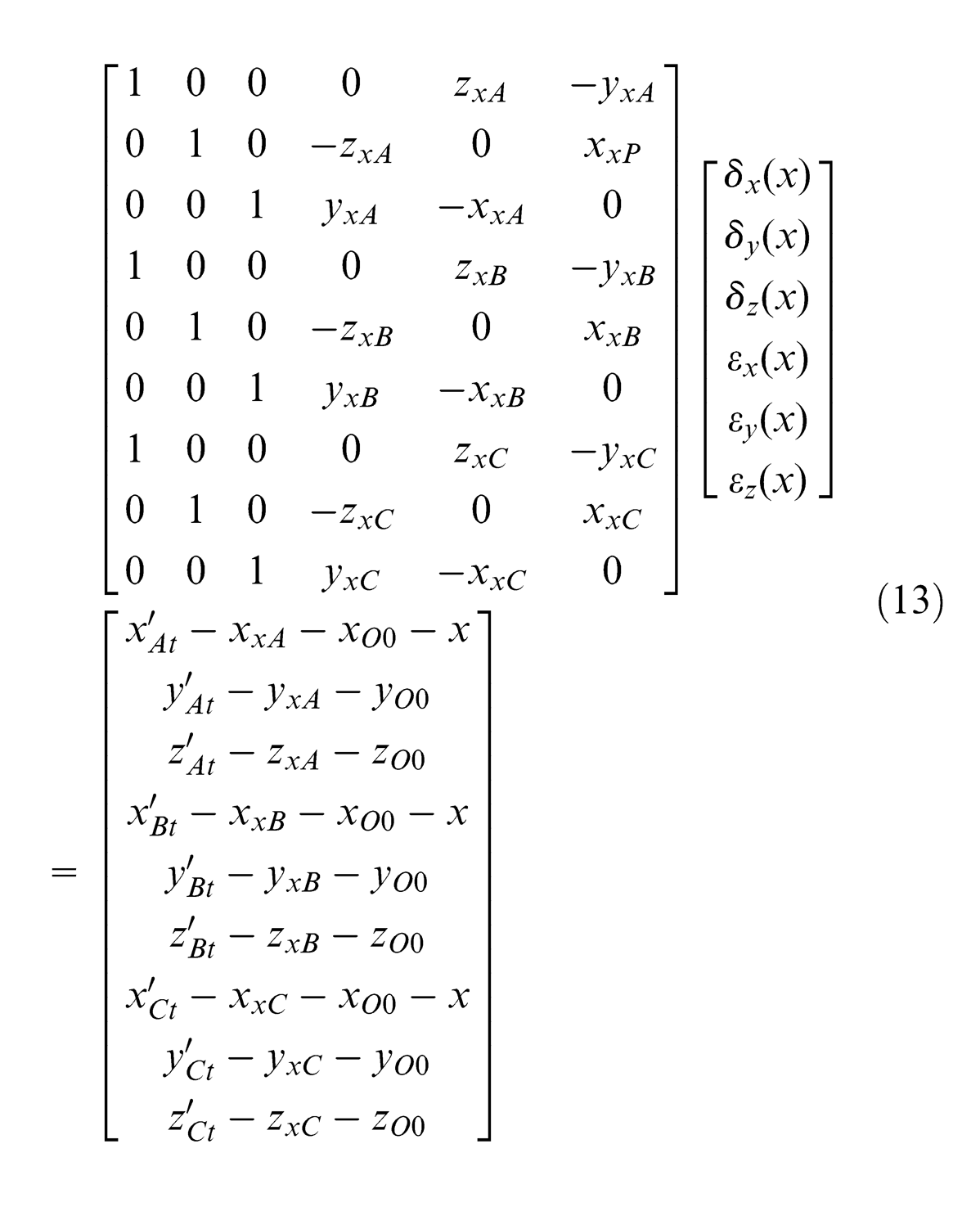
The rank of the coefficient matrix in equation (13) is six if A, B and C are not collinear. So, the three measured points must form a spatial triangle to guarantee the feasibility of this method in the practical application. Least square method is the best way for solving the overdetermined equations in equation (13).
There is also a simple way to calculate the geometric error components, which can avoid the time-consuming iterative computation. Due to that the rank of the coefficient matrix in equation (13) is six if A, B and C are not collinear, so six equations can be reasonably extracted from equation (13) to form a new system of equations which has unique solution. The nine equations in equation (13) can be divided into three sets which are established by analyzing the geometric errors of points A, B and C, respectively, and numbered by a1.a2.a3, b1.b2.b3 and c1.c2.c3, respectively. To guarantee that the new simultaneous equations have solution, this rule should be followed: at least one equation should be extracted from each set, but the combination a1.a2.b1.b2.c1.c2, a1.a3.b1.b3.c1.c3 and a2.a3.b2.b3.c2.c3 cannot be used, that is, the ways of extracting equations from the three sets should not be the same. The combination a1.a2.b1.b3.c2.c3 is used to establish equation (14) in this study
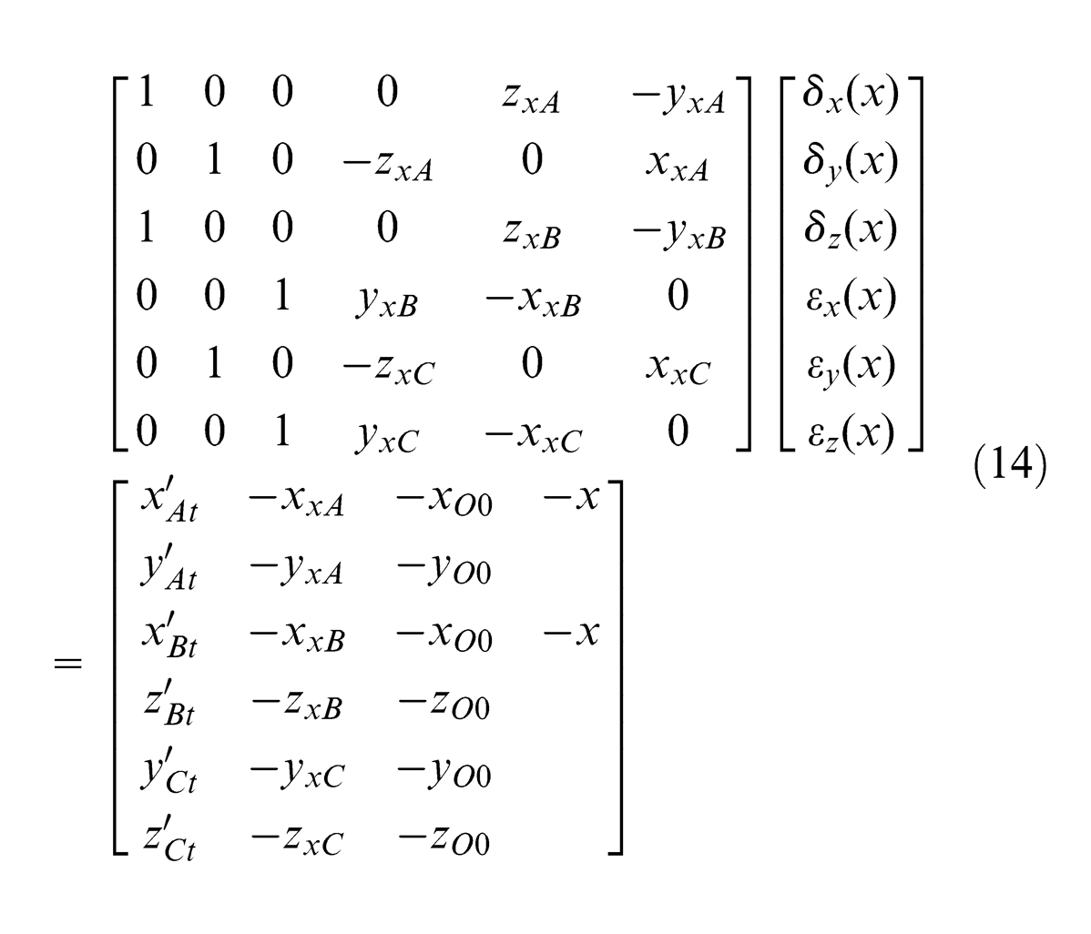
The solution of equation (14) is
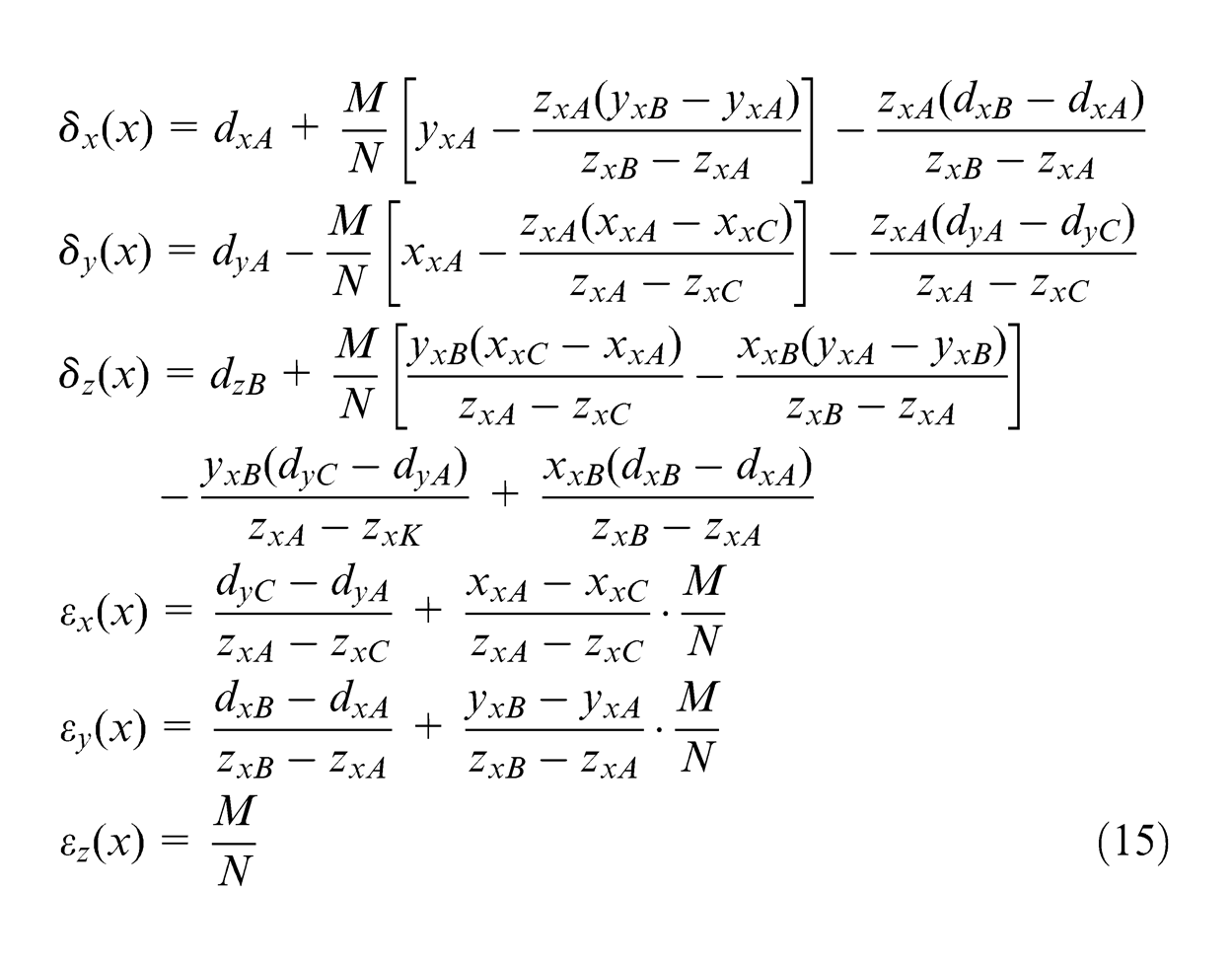
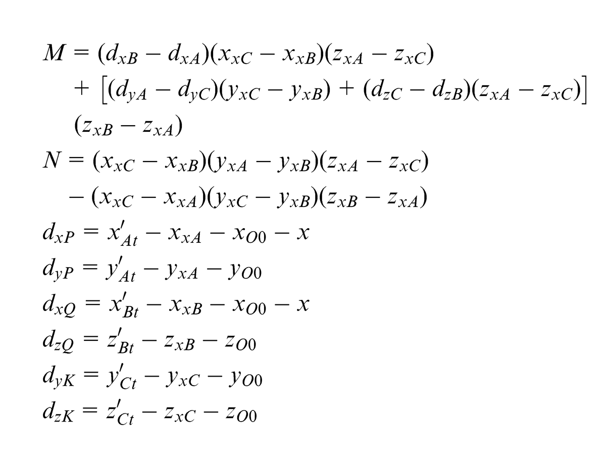
where
Apart from the fact that A, B and C should not be located in a straight line, their relative positions should be reasonably arranged to guarantee that the denominator N in equation (15) not to be zero. The simplest way is to make their z-coordinates not equal to each other. Considering the measurement for x-slide, y-slide and z-slide, the practical measurement should follow the following rule: the c-coordinates (c = x, y or z) of A, B and C are not equal to each other.
Determination of squareness error
First, the RCF is established. As shown in Figure 9, the x-axis of RCF is defined as the average line of x-slide. The x–y plane of RCF is formed by average line of x-slide and y-slide, and the y-axis of RCF lies within x–y plane and is perpendicular to x-axis. The z-axis of RCF is defined as the result of vector product of unit vectors of x-axis and y-axis of RCF. The directions of the three axes of the RCF satisfy the right-hand rule.
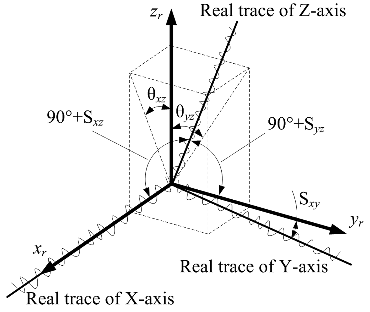
Three squareness errors of three-axis machine tool.
There are totally three squareness errors, Sxy, Sxz and Syz, which are caused by nonorthogonality between the average lines of x-slide, y-slide and z-slide. As shown in Figure 9, Sxy is the rotation angle of the y-slide’s average line about the z-axis of RCF; Sxz and Syz are the rotation angle of z-slide’s average line about the x-axis and y-axis of RCF. θxz and θyz are the projection of Sxz and Syz on the x–z plane and y–z plane. In accordance with the small error hypothesis, θxz and θyz are approximately equal to Sxz and Syz, respectively. The sign symbols of these three squareness errors obey the right-hand rule. Definitely, squareness errors can be computed directly if the locations of every slide’s average line, which is described by linear equations, is known.
The locations of each average line can be obtained by using linear fitting method. For convenience, the offsets between the coordinate frames of adjacent axes are set to zero when all the axes are at the home position. The point A, one point of the three measured points, is considered as the origin of each coordinate frame. Thus, the average line of each axis can be obtained by linear fitting method. Take x-slide as example, assume x-slide totally moves n steps, and the coordinates of the origin is (

Similarly, the mathematical expression of the average lines of y-slide and z-slide are
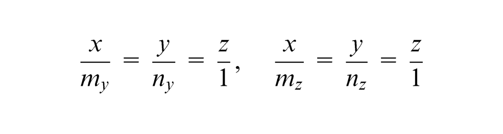
The three squareness errors can be derived from the three directional vectors, that is, (mx, nx, 1), (my, ny, 1) and (mz, nz, 1)
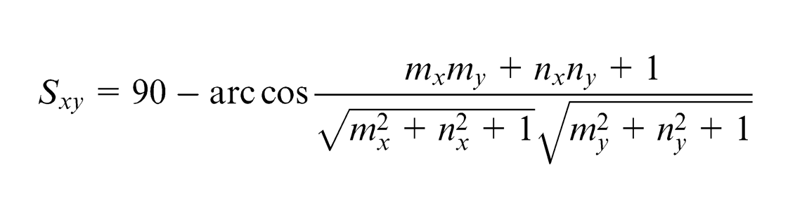
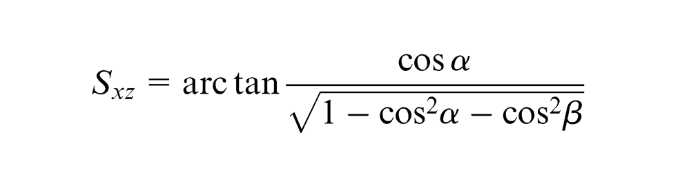
where
Experiments and analysis
Measurement procedure
Take the x-slide as example to demonstrate the measurement procedure.
Step 1. Set up the measuring system—pre-determine the positions of the four additional targets O, Q, K and R by using the method presented in section “Pre-determination of the positions of additional targets,” now xQ, xK, yK, xR, yR and zR are obtained—fix three targets A, B and C on the spindle assembly.
Step 2. Locate the LT at station S1, then place the retroreflector at R and set the reading of LT to zero. Define the distance between the S1 and R to be RAD l1.
Step 3. Measure the incremental distances between S1 and O, Q and K in turn, that is, ΔlO1, ΔlQ1 and ΔlK1.
Step 4. Move x-axis step by step. At the ith step (i = 0, 1, 2, …, nx), measure the incremental distances between S1 and A, B and C, that is, ΔlAi1, ΔlBi1 and ΔlCi1.
Step 5. Repeat Steps 2–4 by locating the LT at S2, and ΔlO2, ΔlQ2, ΔlK2, ΔlAi2, ΔlBi2 and ΔlCi2 can be obtained. Repeat Steps 2–4 by locating the LT at S3, and ΔlO3, ΔlQ3, ΔlK3, ΔlAi3, ΔlBi3 and ΔlCi3 can be obtained. Until now, the measurement procedure is completed.
Step 6. Substitute xQ, xK, yK, xR, yR, zR, ΔlO1, ΔlQ1 and ΔlK1 into equation (6) and solve equation (6) to obtain S1(xS1, yS1, zS1) and l1; substitute xQ, xK, yK, xR, yR, zR, ΔlO2, ΔlQ2 and ΔlK2 into equation (6) and solve equation (6) to obtain S2(xS2, yS2, zS2) and l2 and substitute xQ, xK, yK, xR, yR, zR, ΔlO3, ΔlQ3 and ΔlK3 into equation (6) and solve equation (6) to obtain S3(xS3, yS3, zS3) and l3.
Step 7. Then substitute (xS1, yS1, zS1), (xS2, yS2, zS2), (xS3, yS3, zS3), l1, l2, l3, ΔlAi1, ΔlAi2 and ΔlAi3 into equation (8) and solve equation (8) to obtain Ai(xAi, yAi, zAi); substitute (xS1, yS1, zS1), (xS2, yS2, zS2), (xS3, yS3, zS3), l1, l2, l3, ΔlBi1, ΔlBi2 and ΔlBi3 into equation (8) to obtain Bi(xBi, yBi, zBi) and substitute (xS1, yS1, zS1), (xS2, yS2, zS2), (xS3, yS3, zS3), l1, l2, l3, ΔlCi1, ΔlCi2 and ΔlCi3 into equation (8) to obtain Ci(xCi, yCi, zCi). The coordinates of all the under-test points can be obtained.
Step 8. Substitute all the measured coordinates into equation (13), and then solve equation (13) by least squares method to obtain all the geometric error components of x-slide. Or substitute all the coordinates directly into equation (15) to obtain all the geometric error components.
If a three-axis machine tool is tested, the Steps 2–4 for x-slide, y-slide and z-slide should be conducted successively once the LT is located at a certain Sj, then the Step 5 is conducted, that is, the Steps 2–4 are repeated thrice by locating the LT at three different stations. After all the incremental distance measurements, Steps 6–8 is carried out to obtain the 18 geometric error components of the three linear axes. The three squareness errors are obtained by using the method presented in section “Determination of squareness error.”
The experiments
As shown in Figure 10, a FARO LT is used to measure the 21 geometric error components of a three-axis machine tool of which the type is FXYZ. The strokes of x-axis, y-axis and z-axis are 440, 400 and 400 mm, respectively. Three points A, B and C are fixed on the spindle assembly which moves with a step of 20 mm along with each axis. The coordinates of A, B and C at each step can be determined by using the methods presented in section “Coordinates collection by using LT.” The collected data are first used to establish the RCF, and the three squareness errors can be determined, the results are that Sxy is −22.925 arc sec, Sxz is −27.377 arc sec and Syz is 19.614 arc sec. Meanwhile, the coordinates of every point in the measuring coordinate frame are converted into the coordinates in the corresponding coordinate frame, for example, the coordinates of the measured points are converted to the coordinates in the x-axis coordinate frame during the geometric error components measurement of x-axis. Finally, the equation (13) is solved by using least square method to determine the six geometric error components of each axis, or equation (15) can be applied to determine the six geometric error components of each axis simply. The detailed procedure has been introduced in section “Measurement procedure.” The results are shown in Figure 11.
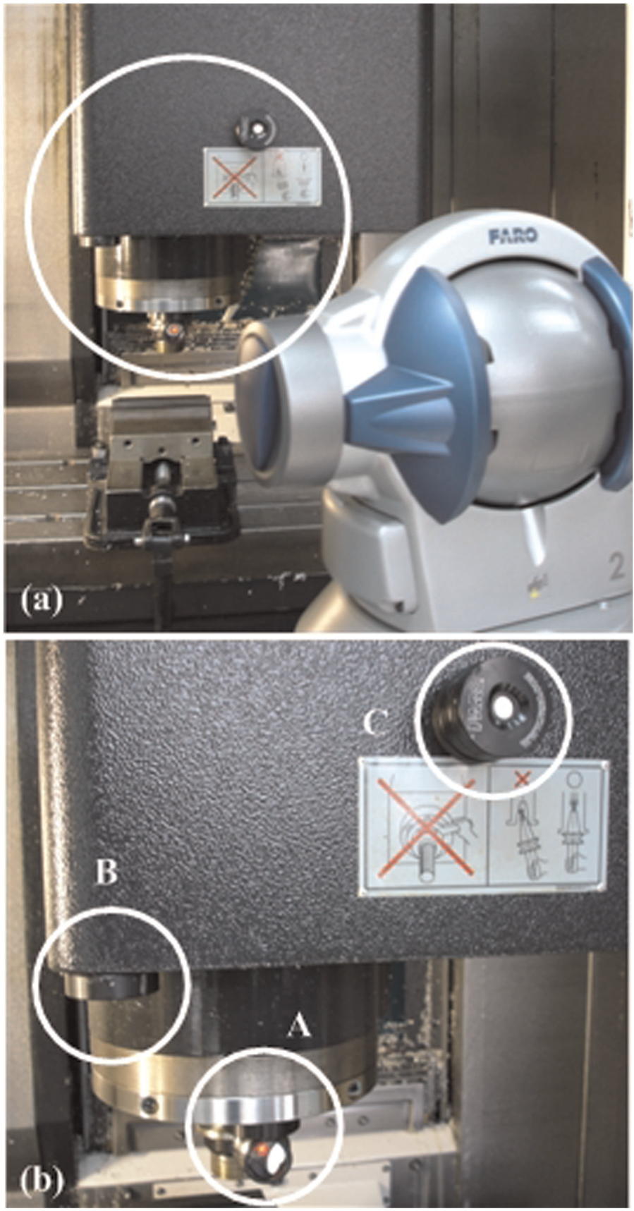
The setup used in experiments: (a) the setup and (b) the arrangement of three points.
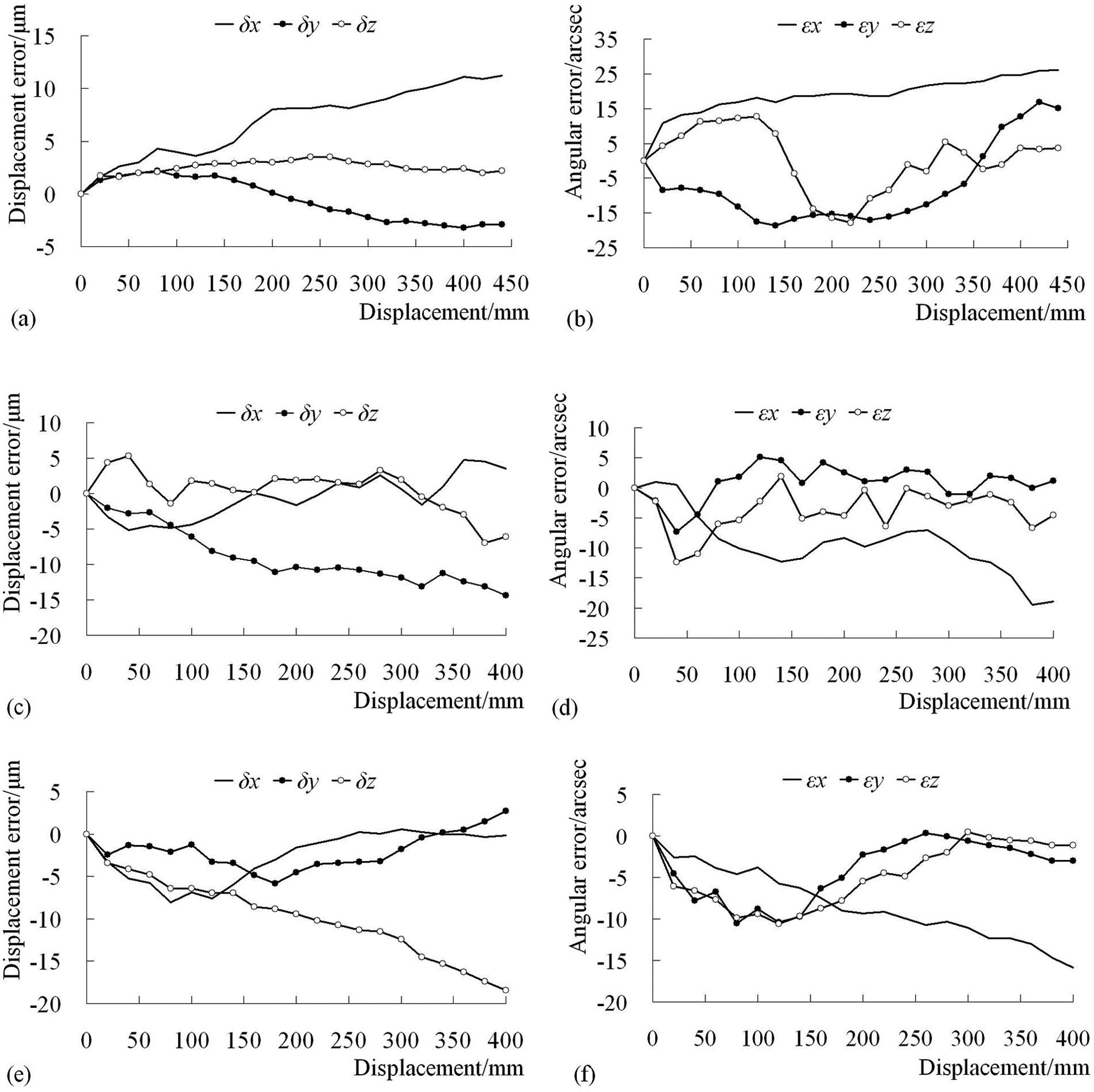
The six geometric error components of each axis: (a) three displacement errors of x-axis, (b) three angular errors of x-axis, (c) three displacement errors of y-axis, (d) three angular errors of y-axis, (e) three displacement errors of z-axis and (f) three angular errors of z-axis.
In this article, the software compensation is applied to realize the volumetric error compensation of machine tool. First, the geometric error components which have been obtained by experiments are saved into the computer as the format of a table. The recursive error compensation technique 14 is applied to decrease the volumetric error, that is, use the equation (5a), (5b) and (5c) to compute the volumetric error recursively, and enable the spindle assembly to reach the desired position as close as possible. If the desired position is not located at one of the positions sampled during the geometric error components measurement, the interpolation is applied to obtain the volumetric errors of the desired position. Laser interferometer is acknowledged as a high-accuracy equipment for machine tool calibration. As shown in Figure 12, an experiment is conducted to measure the positioning errors when the machine tool moves along the x-axis, y-axis and z-axis, respectively, with a laser interferometer in the case of without compensation and with compensation. The coordinate of the measured point is T(175.6, 497.5, 312.1) when the machine tool is at the home position. What should be emphasized is that the displacements of three axis which are substituted into equation (5a), (5b) and (5c) should be (x+175.6), (y+497.5) and (z+312.1) mm, respectively, and that the length of tool, l is set to zero. The sample interval is 10 mm. The experimental results are illustrated in Figure 13.
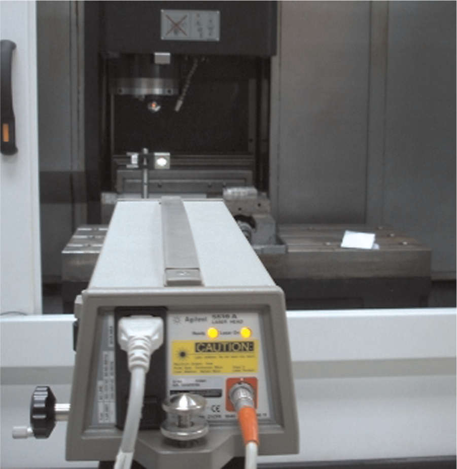
Measuring positioning errors by using laser interferometer.
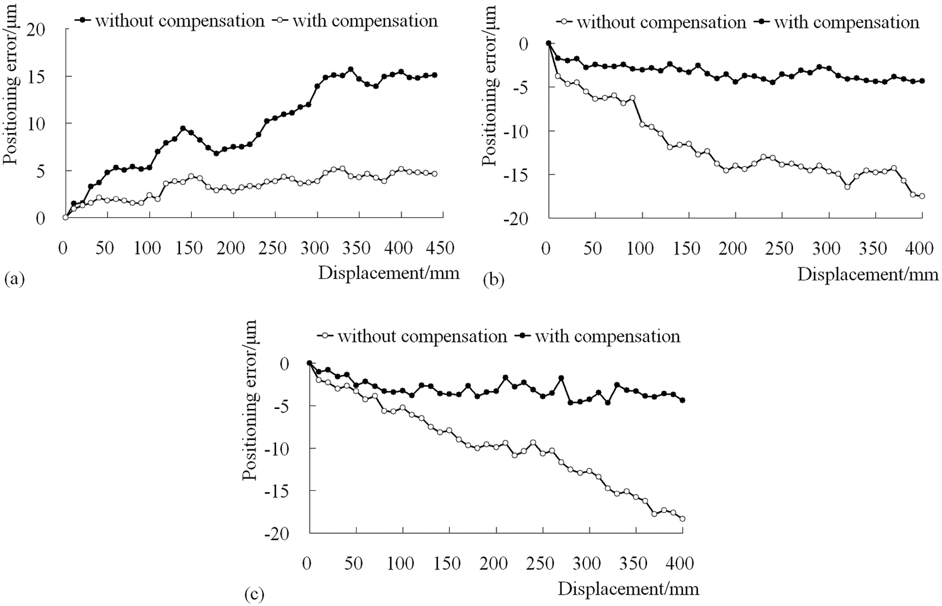
Results of comparison experiments: (a) the positioning error along x-axis, (b) the positioning error along y-axis and (c) the positioning error along z-axis.
According to results of experiments, the position errors of point T along three axes are significantly reduced. Concretely, the maximum errors along x-axis are reduced from 16.69 to 5.11 µm, the maximum errors along y-axis are reduced from −17.52 to −4.47 µm and the maximum errors along z-axis are reduced from −18.38 to −4.67 µm. The experimental results demonstrate that the error compensation can enhance the accuracy of machine tool, and that the presented method for the geometric error components measurement is effective.
Conclusion
A three-point method for measuring geometric error of three-axis machine tools using LT has been presented in this study. The 21 geometric error components can be measured by using only one LT to collect the coordinate sequence of three points along with three axes in the workspace of the machine tools, and then, the volumetric errors can be obtained by substituting the 21 geometric error components into the error model of three-axis machine tool rather than directly measuring the volumetric errors of sample nodes in the whole workspace. The experiments are conducted to determine all the 21 geometric error components, and the volumetric error compensation is also conducted by using a recursive error compensation technique. A laser interferometer is used to test the positioning errors of each axis in the case of without compensation and with compensation, the results of which can validate the effectiveness of the presented method for geometric error measurement and compensation.
Since there is no requirement of complicated equipment alignment, the presented method is simple and fast; furthermore, it does not require experienced operators. All the geometric errors of three-axis can be verified successfully within 3 h, including the time consumed in pre-determining the positions of the additional targets based on sequential multilateration principle. This method is suitable for the geometric error measurement of different-sized machine tools, and due to the large-scale 3D coordinate measurement capability of the LTs, it is especially suitable for geometric error measurement of large-scale machine tool. In addition, the measurements are performed in a single coordinate system rather than three axes or many lines, that is, all the coordinates are measured in the same measuring coordinate frame, so that the errors induced by transforming the coordinate frames can be avoided.
Footnotes
Acknowledgements
The authors would like to express their appreciation to Wang Ying and Liu Nengfeng, who are the assistant engineers at Shenzhen Key Laboratory of Advanced Manufacturing Technology of Harbin Institute of Technology Shenzhen Graduate School, for offering their help to accomplish the experiments.
Declaration of conflicting interests
The authors declare that there is no conflict of interest.
Funding
This work was supported in part by National Natural Science Foundation of China (NSFC) under NSFC Grant 60974069.